Fixed-time Synchronization of Networked Uncertain Euler-Lagrange Systems

Yi Dong and Zhiyong Chen This work has been supported in part by Shanghai Municipal Science and Technology Major Project under grant 2021SHZDZX0100, in part by National Natural Science Foundation of China under grant 62073241 and in part by the Fundamental Research Funds for the Central Universities under grant 22120210127.Y. Dong is with College of Electronic and Information Engineering, Tongji University, Shanghai 200092, China. Email: yidong@tongji.edu.cnZ. Chen is with with the School of Electrical Engineering and Computing, The University of Newcastle, Callaghan, NSW 2308, Australia. E-mail: zhiyong.chen@newcastle.edu.au

Abstract

This paper considers the fixed-time control problem of a multi-agent system composed of a class of Euler-Lagrange dynamics with parametric uncertainty and a dynamic leader under a directed communication network. A distributed fixed-time observer is first proposed to estimate the desired trajectory and then a fixed-time controller is constructed by transforming uncertain Euler-Lagrange systems into second-order systems and utilizing the backstepping design procedure. The overall design guarantees that the synchronization errors converge to zero in a prescribed time independent of initial conditions. The control design conditions can also be relaxed for a weaker finite-time control requirement.

Index Terms:

Finite-time control, fixed-time control, multi-agent systems, Euler-Lagrange systems, directed graph

I Introduction

Fixed-time control for multi-agent systems, requiring exact achievement of a collective behavior in a prescribed time independent of initial conditions, or finite-time control of a weaker requirement allowing the prescribed time dependent on initial conditions, has attracted researchers’ extensive attention over the past years due to its potential advantages in transient performance and robustness property [1]. The early work on finite-time formation control of single-integrator multi-agent systems can be found in [2]. For the leader-following consensus problem of general linear multi-agent systems, [3] proposed two classes of finite-time observers to estimate the second-order leader dynamics, which can work in undirected and directed communication networks, respectively. More efforts have also been devoted to nonlinear systems. For example, [4] considered the finite-time control of first-order multi-agent systems with unknown nonlinear dynamics, while both first-order and second-order nonlinear systems were considered in[5]. In particular, observer-based control was proposed to solve the leader-following fixed-time consensus problem under the strongly connected communication network. The fixed-time consensus problem was also investigated for double-integrator systems under directed communication network and more general multi-agent systems with high-order integrator dynamics in [6, 7], respectively.

Euler-Lagrange systems capture a large class of contemporary engineering problems and finite-time control of this class of systems has been intensively investigated, especially in the individual setting. For example, [8] considered finite-time control for an Euler-Lagrange system based on the method for a double-integrator system, while [9, 10] further dealt with nonlinear systems in the presence of uncertainties. The work in [11] studied a non-singular sliding surface and constructed a continuous finite-time control strategy for uncertain Euler-Lagrange system. Furthermore, [12] designed an adaptive controller to track a desired trajectory in finite time and [13] proposed a method for handing both uncertain dynamics and globally unbounded disturbances.

The research on fixed-time or finite-time control of uncertain Euler-Lagrange systems in a network setting is relatively rare. Some related results can be found in [14] where, by adaptive control technique, a finite-time synchronization controller was constructed for a multi-agent system modeled by some mechanical nonlinear systems with a connected communication network. The recent work reported in [15] studied finite-time coordination behavior of a multiple Euler-Lagrange system with an undirected network in the absence of uncertainties. In particular, with the introduction of auxiliary variables, the system can be converted into a simpler form such that the adding a power integrator method can be applied to ensure the convergence.

This paper provides a solution to the leader-following fixed-time synchronization problem for multiple Euler-Lagrange systems with parametric uncertainty. The strategy is based on a class of observers that can accurately estimate a dynamic trajectory in a fixed time. The design relaxes the undirected and connected assumption for the communication network in [5, 7, 14, 15] and considers a directed network graph. Then an observer-based controller is proposed for the multi-agent system composed of a dynamic leader and multiple heterogeneous Euler-Lagrange dynamics, as opposed to the finite-time control method for multiple special mechanical systems in [14]. In particular, the distributed control law is able to guarantee each Euler-Lagrange system can track a desired trajectory in a prescribed time, independent of initial conditions. It is worth mentioning that the control design conditions can be relaxed for a weaker finite-time control requirement. Also, a reduced continuous controller can be directly applied to the fixed-time synchronization problem for second-order nonlinear systems with a directed graph.

Throughout the paper, we use the following notations. For a vector $x=[x_{1},\cdots,x_{n}]^{T}\in\mathbb{R}^{n}$ , $\|x\|_{1}=|x_{1}|+\cdots+|x_{n}|$ represents its Manhattan ( ${\cal L}_{1}$ ) norm, $\|x\|=\sqrt{x_{1}^{2}+\cdots,x_{n}^{2}}$ its Euclidean ( ${\cal L}_{2}$ ) norm, and $|x|=[|x_{1}|,\cdots,|x_{n}|]^{T}$ its element-wise absolute valued vector. For a matrix $X$ , $|X|$ is also defined as its element-wise absolute valued matrix. The power function operator is element-wise in terms of $x^{a}=[x^{a}_{1},\cdots,x^{a}_{n}]^{T}$ for $a>0$ . For two vectors (matrices) $X$ and $Y$ , comparison operators are element-wise; for example, $X\geq Y$ means $x_{ij}\geq y_{ij}$ for every $x_{ij}$ and $y_{ij}$ , the $(i,j)$ -elements of $X$ and $Y$ , respectively. The operator $\mbox{sig}^{a}(x)=[\mbox{sign}(x_{1})|x_{1}|^{a},\cdots,\mbox{sign}(x_{n})|x_{n}|^{a}]^{T}$ is defined for $a>0$ and the sign function $\mbox{sign}(\cdot)$ .

II Problem Formulation

Consider a group of $m$ -link robotic manipulators of the following Euler-Lagrange dynamics

\displaystyle M_{i}(q_{i})\ddot{q}_{i}+C_{i}(q_{i},\dot{q}_{i})\dot{q}_{i}+G_{i}(q_{i})=\tau_{i},\;i=1,\cdots,N,

(1)

where $q_{i}\in\mathbb{R}^{m}$ , $\dot{q}_{i}\in\mathbb{R}^{m}$ are the vectors of generalized position and velocity of the $i$ -th robotic manipulator, also called agent $i$ , $M_{i}(q_{i})\in\mathbb{R}^{m\times m}$ is a symmetric and positive definite inertia matrix, $C_{i}(q_{i},\dot{q}_{i})\dot{q}_{i}\in\mathbb{R}^{m}$ contains the Coriolis and centrifugal forces, $G_{i}(q_{i})\in\mathbb{R}^{m}$ is the gravitational torque, and $\tau_{i}\in\mathbb{R}^{m}$ is the vector of control force. The reference is generated by a leader system, called agent 0, described as follows:

\displaystyle\dot{\eta}_{0}

\displaystyle=S\eta_{0},\;q_{0}=E\eta_{0},

(2)

where $\eta_{0}\in\mathbb{R}^{n}$ is the state, $q_{0}\in\mathbb{R}^{m}$ is the desired trajectory to track, and $S\in\mathbb{R}^{n\times n}$ , $E\in\mathbb{R}^{m\times n}$ are constant matrices.

The multi-agent system under consideration is composed of the $N$ dynamics in (1) and the dynamic leader (2). The information flow among all the $N+1$ agents is described by a digraph $\mathcal{G}=(\mathcal{V},\mathcal{E})$ where $\mathcal{V}=\{0,1,\cdots,N\}$ is the node set and $\mathcal{E}\subset\mathcal{V}\times\mathcal{V}$ is the edge set. Each element $(j,i)\in\mathcal{E}$ represents the edge from agent $j$ to agent $i$ . For $i,j\in\mathcal{V}$ , $a_{ii}=0$ , $a_{ij}>0$ if $(j,i)\in\mathcal{E}$ and $a_{ij}=0$ otherwise. Let $H=[h_{ij}]_{i,j=1}^{N}$ be the Laplacian matrix of the subnetwork composed of agents $1,\cdots,N$ , where $h_{ii}=\sum_{j=0}^{N}a_{ij}$ and $h_{ij}=-a_{ij}$ for $i\neq j$ , $i,j=1,\cdots,N$ .

The objective of this paper is to design a distributed control law such that each agent of (1) can track the desired trajectory $q_{0}$ in fixed time. More specifically, we consider the class of control laws of the form

	$\displaystyle\tau_{i}$	$\displaystyle=f_{1i}(q_{i},\dot{q}_{i},\eta_{i},\dot{\eta}_{i})$
	$\displaystyle\dot{\eta}_{i}$	$\displaystyle=f_{2i}(\eta_{i},\sum_{j=0}^{N}a_{ij}(\eta_{i}-\eta_{j})),\;i=1,\cdots,N.$		(3)

Let

\displaystyle x_{i}=\left[\begin{array}[]{c}q_{i}-q_{0}\\ \dot{q}_{i}-\dot{q}_{0}\\ \eta_{i}-\eta_{0}\end{array}\right],i=1,\cdots,N,\;x=\left[\begin{array}[]{c}x_{1}\\ \vdots\\ x_{N}\end{array}\right]\in\mathbb{R}^{n_{x}}.

Suppose the closed-loop system composed of (1), (2) and (3) possesses unique solutions in forward time for all initial conditions. Then the fixed-time synchronization problem can be described as follows based on the concept of fixed-time stability [16].

Fixed-time synchronization problem: Given the system composed of (1) and (2) with the corresponding digraph $\mathcal{G}$ , design a distributed control law of the form (3) such that, for all initial conditions $x(0)=x_{0}$ and $\eta_{0}(0)=\eta_{00}$ , the equilibrium $x=0$ of the closed-loop system is (globally) fixed-time stable. That is, the solution $x(t)$ exists for $t\geq 0$ and $x=0$ is Lyapunov stable, and moreover, there exists a fixed time $T^{*}$ , independent of $x_{0}$ or $\eta_{00}$ , such that

	$\displaystyle\lim_{t\rightarrow T^{*}}x(t)=0,$
	$\displaystyle x(t)=0,\;t\geq T^{*},\;\forall x_{0}\in\mathbb{R}^{n_{x}},\eta_{00}\in\mathbb{R}^{n}.$		(4)

Remark II.1

When the existence of a fixed time $T^{*}$ is relaxed to the existence of a settling-time function $T(x_{0},\eta_{00})$ , the above fixed-time synchronization problem is called a finite-time synchronization problem, which is based on the definition of finite-time stability [1]. In practice, there is similarity between finite-time convergence and asymptotical (exponential) convergence, both of which require the convergence of trajectories to (proximity of) an equilibrium point in a finite amount of time which depends on the initial conditions. But fixed-time convergence is a more practically interesting feature which requests it happen in a prescribed time independent of initial conditions. There are more constraints on the controller design conditions that will be studied in this paper.

For the solvability of the aforementioned problem, we need the following standard assumption on the communication network.

Assumption II.1

The graph $\mathcal{G}$ contains a spanning tree with node 0 as the root.

Remark II.2

Under Assumption II.1, all the eigenvalues of $H$ have positive real parts; see, e.g., [17]. By Theorem 2.5.3 of [18], there exists a positive definite diagonal matrix $\bar{D}\in\mathbb{R}^{N\times N}$ such that $H^{T}\bar{D}+\bar{D}H$ is positive definite. Let $\lambda_{m}>0$ be the smallest eigenvalue of $H^{T}\bar{D}+\bar{D}H$ and $D=\mbox{diag}(d_{1},\cdots,d_{N})=2\bar{D}/\lambda_{m}$ . One has $H^{T}D+DH\geq 2I_{N}$ .

We end this section with some technical lemmas from, e.g., [6], [16], [19] and [20], which will be used in the proofs of the main results in this paper.

Lemma II.1

For any $\xi_{i}\in\mathbb{R}$ , $i=1,\cdots,n$ , and any $p\in(0,1]$ , $(\sum_{i=1}^{n}|\xi_{i}|)^{p}\leq\sum_{i=1}^{n}|\xi_{i}|^{p}\leq n^{1-p}(\sum_{i=1}^{n}|\xi_{i}|)^{p}$ [19]. For any $p>1$ , $\sum_{i=1}^{n}|\xi_{i}|^{p}\leq(\sum_{i=1}^{n}|\xi_{i}|)^{p}\leq n^{p-1}\sum_{i=1}^{n}|\xi_{i}|^{p}$ [6].

Lemma II.2

[19] The inequality $|\xi_{i}^{p}-\xi_{j}^{p}|\leq 2^{1-p}|\xi_{i}-\xi_{j}|^{p}$ holds for $\forall\xi_{i},\xi_{j}\in\mathbb{R}$ and $0<p\leq 1$ and $p$ is a ratio of two odd integers.

Lemma II.3

[20] The inequality $|\xi_{i}|^{c}|\xi_{j}|^{d}\leq\frac{c}{c+d}r|\xi_{i}|^{c+d}+\frac{d}{c+d}r^{-\frac{c}{d}}|\xi_{j}|^{c+d}$ holds for $\forall\xi_{i},\xi_{j}\in\mathbb{R}$ and $c,d,r>0$ .

Lemma II.4

(Lemma 1, [16]) Consider the system $\dot{z}=\phi(z,t)$ where $\phi:\mathbb{R}^{l}\times[0,\infty)\mapsto\mathbb{R}^{l}$ satisfies $\phi(0,t)=0$ . Suppose there exits a continuously differentiable function $V:~{}\mathbb{R}^{l}\mapsto\mathbb{R}$ such that (i) $V$ is positive definite and proper; and (ii) there exist real numbers $p_{0},q_{0},p,q,k>0$ with $pk<1$ and $qk>1$ such that $\dot{V}(z)\leq-(p_{0}(V(z))^{p}+q_{0}(V(z))^{q})^{k}$ . Then, the equilibrium $z=0$ is (globally) fixed-time stable and there is a constant settling-time $T^{*}\leq\frac{1}{p_{0}^{k}(1-pk)}+\frac{1}{q_{0}^{k}(qk-1)}$ .

III Distributed observer design

As the agents not connected to agent 0 do not have access to the information of the dynamic leader (2), its state needs to be estimated by a properly designed fixed-time observer as follows:

	$\displaystyle\dot{\eta}_{i}$	$\displaystyle=S\eta_{i}-c_{1}y_{i}-c_{2}\mbox{sig}^{a}(y_{i})-c_{3}\mbox{sig}^{b}(y_{i}),$
	$\displaystyle y_{i}$	$\displaystyle=\sum_{j=0}^{N}a_{ij}(\eta_{i}-\eta_{j}),\;i=1,\cdots,N.$		(5)

In this section, we construct a lemma based on the fixed-time observer (III). Let $\eta^{T}=[\eta^{T}_{0},\eta^{T}_{1},\cdots,\eta^{T}_{N}]^{T}$ for the convenience of presentation.

Lemma III.1

Consider the system composed of (2) and (III) under Assumption II.1 with $0<a<1$ , $b>\frac{1}{a}>1$ , $c_{1}>\|D\otimes S\|$ and $c_{2},c_{3}>0$ . There exists a constant settling-time $T^{*}_{1}\geq 0$ such that, $\forall\eta(0)\in\mathbb{R}^{(N+1)n}$ ,

	$\displaystyle\lim_{t\rightarrow T_{1}^{*}}(\eta_{i}(t)-\eta_{0}(t))=0,$
	$\displaystyle\eta_{i}(t)-\eta_{0}(t)=0,\;t\geq T_{1}^{*},\;i=1,\cdots,N.$		(6)

Proof: Let $\bar{\eta}_{i}=\eta_{i}-\eta_{0}$ , $i=0,1,\cdots,N$ . The observer (III) can be rewritten as

	$\displaystyle\dot{\bar{\eta}}_{i}$	$\displaystyle=S\bar{\eta}_{i}-c_{1}y_{i}-c_{2}\mbox{sig}^{a}(y_{i})-c_{3}\mbox{sig}^{b}(y_{i}),$
	$\displaystyle y_{i}$	$\displaystyle=\sum_{j=0}^{N}a_{ij}(\bar{\eta}_{i}-\bar{\eta}_{j}),\;i=1,\cdots,N.$		(7)

Let $Y_{i}=c_{1}y_{i}+c_{2}\mbox{sig}^{a}(y_{i})+c_{3}\mbox{sig}^{b}(y_{i})$ and $\bar{\eta}$ , $y$ , $Y$ be the column stacks of $\bar{\eta}_{i}$ , $y_{i}$ , $Y_{i}$ , $i=1,\cdots,N$ . Note $y=(H\otimes I_{n})\bar{\eta}$ and

\dot{y}=(I_{N}\otimes S)y-(H\otimes I_{n})Y.

(8)

And, let

	$\displaystyle V(y)=$	$\displaystyle\sum_{i=1}^{N}\left(\frac{c_{2}d_{i}}{1+a}\\|y_{i}^{1+a}\\|_{1}+\frac{c_{3}d_{i}}{1+b}\\|y_{i}^{1+b}\\|_{1}\right)$
		$\displaystyle+\frac{c_{1}}{2}y^{T}(D\otimes I_{n})y.$		(9)

Along the trajectory of (8), the time derivative of $V(y)$ satisfies

	$\displaystyle\dot{V}(y)=$	$\displaystyle\sum_{i=1}^{N}d_{i}(c_{2}\mbox{sig}^{a}(y_{i})+c_{3}\mbox{sig}^{b}(y_{i}))^{T}\dot{y}_{i}+c_{1}y^{T}(D\otimes I_{n})\dot{y}$
	$\displaystyle=$	$\displaystyle Y^{T}(D\otimes I_{n})\dot{y}$
	$\displaystyle=$	$\displaystyle Y^{T}(D\otimes S)y-\frac{1}{2}Y^{T}((H^{T}D+DH)\otimes I_{n})Y$
	$\displaystyle\leq$	$\displaystyle\frac{1}{2}Y^{T}Y+\frac{1}{2}\\|D\otimes S\\|^{2}y^{T}y-Y^{T}Y$
	$\displaystyle=$	$\displaystyle-\frac{1}{2}(\\|Y\\|^{2}-\\|D\otimes S\\|^{2}\\|y\\|^{2}).$

Further calculation shows that

	$\displaystyle\\|Y_{i}\\|^{2}=$	$\displaystyle\\|c_{1}y_{i}+c_{2}\mbox{sig}^{a}(y_{i})+c_{3}\mbox{sig}^{b}(y_{i}))\\|^{2}$
	$\displaystyle\geq$	$\displaystyle c_{1}^{2}\\|y_{i}\\|^{2}+c_{2}^{2}\\|\mbox{sig}^{a}(y_{i})\\|^{2}+c_{3}^{2}\\|\mbox{sig}^{b}(y_{i})\\|^{2}$
	$\displaystyle\geq$	$\displaystyle c_{1}^{2}\\|y_{i}\\|^{2}+c_{2}^{2}\\|y_{i}^{2a}\\|_{1}+c_{3}^{2}\\|y_{i}^{2b}\\|_{1}.$

By Lemma II.1, for $0<a<1$ and $b>1$ ,

	$\displaystyle\sum_{i=1}^{N}\\|y_{i}^{2a}\\|_{1}\geq(\sum_{i=1}^{N}\\|y_{i}^{2}\\|_{1})^{a}=(\\|y\\|^{2})^{a},$
	$\displaystyle\sum_{i=1}^{N}\\|y_{i}^{2b}\\|_{1}\geq\frac{1}{(nN)^{b-1}}(\\|y\\|^{2})^{b}.$

As a result,

\displaystyle\|Y\|^{2}=

\displaystyle\sum_{i=1}^{N}\|Y_{i}\|^{2}\geq c_{1}^{2}\|y\|^{2}+c_{2}^{2}(\|y\|^{2})^{a}+\frac{c_{3}^{2}}{(nN)^{b-1}}(\|y\|^{2})^{b}

and hence

$\displaystyle\dot{V}(y)\leq$	$\displaystyle-\frac{1}{2}(c_{1}^{2}-\\|D\otimes S\\|^{2})\\|y\\|^{2}-\frac{c_{2}^{2}}{2}(\\|y\\|^{2})^{a}$
	$\displaystyle-\frac{c_{3}^{2}}{2(nN)^{b-1}}(\\|y\\|^{2})^{b}$
$\displaystyle\leq$	$\displaystyle-\hat{c}_{1}\left(\\|y\\|^{2}+(\\|y\\|^{2})^{a}+(\\|y\\|^{2})^{b}\right)$	(10)

for

\displaystyle\hat{c}_{1}=\min\left\{\frac{1}{2}(c_{1}^{2}-\|D\otimes S\|^{2}),\frac{c_{2}^{2}}{2},\frac{c_{3}^{2}}{2(nN)^{b-1}}\right\}>0.

Analysis on (9) using Lemma II.1 and noting $0<\frac{2a}{1+a}<1$ and $\frac{a(1+b)}{1+a}>1$ gives

	$\displaystyle V^{\frac{2a}{1+a}}\leq$	$\displaystyle\sum_{i=1}^{N}\Big{(}(\frac{c_{1}d_{i}}{2})^{\frac{2a}{1+a}}\\|y_{i}^{\frac{4a}{1+a}}\\|_{1}+(\frac{c_{2}d_{i}}{1+a})^{\frac{2a}{1+a}}\\|y_{i}^{2a}\\|_{1}$
		$\displaystyle+(\frac{c_{3}d_{i}}{1+b})^{\frac{2a}{1+a}}\\|y_{i}^{\frac{2a(1+b)}{1+a}}\\|_{1}\Big{)}$
	$\displaystyle\leq$	$\displaystyle\hat{c}_{2}\left((\\|y\\|^{2})^{\frac{2a}{1+a}}+(\\|y\\|^{2})^{a}+(\\|y\\|^{2})^{\frac{a(1+b)}{1+a}}\right)$

for $d_{\max}=\max\{d_{1},\cdots,d_{N}\}$ and

	$\displaystyle\hat{c}_{2}=$	$\displaystyle\max\Big{\{}(\frac{c_{1}d_{\max}}{2})^{\frac{2a}{1+a}}(nN)^{1-\frac{2a}{1+a}},$
		$\displaystyle(\frac{c_{2}d_{\max}}{1+a})^{\frac{2a}{1+a}}(nN)^{1-a},(\frac{c_{3}d_{\max}}{1+b})^{\frac{2a}{1+a}}\Big{\}}.$

Since $a<\frac{2a}{1+a}<1$ and $a<\frac{a(1+b)}{1+a}<b$ , we can easily verify

	$\displaystyle(\\|y\\|^{2})^{\frac{2a}{1+a}}\leq$	$\displaystyle\\|y\\|^{2}+(\\|y\\|^{2})^{a}$
	$\displaystyle(\\|y\\|^{2})^{\frac{a(1+b)}{1+a}}\leq$	$\displaystyle(\\|y\\|^{2})^{a}+(\\|y\\|^{2})^{b}$

and hence

\displaystyle V^{\frac{2a}{1+a}}\leq

\displaystyle\hat{c}_{2}\left(\|y\|^{2}+3(\|y\|^{2})^{a}+(\|y\|^{2})^{b}\right).

(11)

Similarly, for $b>1$ , $\frac{2b}{1+b}>1$ and $\frac{b(1+a)}{1+b}>1$ ,

\displaystyle V^{\frac{2b}{1+b}}

\displaystyle\leq\hat{c}_{3}\left((\|y\|^{2})^{\frac{2b}{1+b}}+(\|y\|^{2})^{\frac{b(1+a)}{1+b}}+(\|y\|^{2})^{b}\right)

for

	$\displaystyle\hat{c}_{3}=$	$\displaystyle\max\left\{(\frac{c_{1}d_{\max}}{2})^{\frac{2b}{1+b}},~{}(\frac{c_{2}d_{\max}}{1+a})^{\frac{2b}{b+1}},(\frac{c_{3}d_{\max}}{1+b})^{\frac{2b}{b+1}}\right\}$
		$\displaystyle\times(3nN)^{\frac{b-1}{b+1}}.$

Since $1<\frac{2b}{1+b}<b$ and $a<\frac{b(1+a)}{1+b}<b$ , we can easily verify

	$\displaystyle(\\|y\\|^{2})^{\frac{2b}{1+b}}\leq$	$\displaystyle\\|y\\|^{2}+(\\|y\\|^{2})^{b}$
	$\displaystyle(\\|y\\|^{2})^{\frac{b(1+a)}{1+b}}\leq$	$\displaystyle(\\|y\\|^{2})^{a}+(\\|y\\|^{2})^{b}$

and hence

\displaystyle V^{\frac{2b}{1+b}}\leq

\displaystyle\hat{c}_{3}\left(\|y\|^{2}+(\|y\|^{2})^{a}+3(\|y\|^{2})^{b}\right)

(12)

Finally, by (11) and (12), one has

\displaystyle\frac{1}{\hat{c}_{2}}V^{\frac{2a}{1+a}}+\frac{1}{\hat{c}_{3}}V^{\frac{2b}{1+b}}\leq 4\left(\|y\|^{2}+(\|y\|^{2})^{a}+(\|y\|^{2})^{b}\right),

which, compared with (10), implies

\displaystyle\dot{V}\leq-\frac{\hat{c}_{1}}{4\hat{c}_{2}}V^{\frac{2a}{1+a}}-\frac{\hat{c}_{1}}{4\hat{c}_{3}}V^{\frac{2b}{1+b}}.

By Lemma II.4, the system (8) is fixed-time stable. In particular, there exists a constant

\displaystyle T_{1}^{*}\leq\frac{4\hat{c}_{2}(a+1)}{\hat{c}_{1}(1-a)}+\frac{4\hat{c}_{3}(b+1)}{\hat{c}_{1}(b-1)},

such that $\lim_{t\rightarrow T_{1}^{*}}y(t)=0$ and $y(t)=0$ , $t\geq T_{1}^{*}$ . Under Assumption II.1, we have $\bar{\eta}=(H^{-1}\otimes I_{n})y$ and hence (6). The proof is thus completed. $\Box$

Remark III.1

When $c_{3}=0$ , the observer (III) reduces to a finite-time observer

	$\displaystyle\dot{\eta}_{i}$	$\displaystyle=S\eta_{i}-c_{1}y_{i}-c_{2}\mbox{sig}^{a}(y_{i}),$
	$\displaystyle y_{i}$	$\displaystyle=\sum_{j=0}^{N}a_{ij}(\eta_{i}-\eta_{j}),\;i=1,\cdots,N.$		(13)

Consider the system composed of (2) and (III.1) under Assumption II.1 with $0<a<1$ , $c_{1}>\|D\otimes S\|$ and $c_{2}>0$ . There exists a settling-time function $T_{1}(\eta(0))\geq 0$ such that, $\forall\eta(0)\in\mathbb{R}^{(N+1)n}$ ,

	$\displaystyle\lim_{t\rightarrow T_{1}}(\eta_{i}(t)-\eta_{0}(t))=0,\;i=1,\cdots,N$
	$\displaystyle\eta_{i}(t)-\eta_{0}(t)=0,\;t\geq T_{1}(\eta(0)).$		(14)

The proof of the above statement follows that of Lemma III.1 using simple arguments. In particular, we can obtain

\displaystyle\dot{V}\leq-\frac{\hat{c}_{1}}{3\hat{c}_{2}}V^{\frac{2a}{1+a}}.

In other words, $\dot{V}+\varrho V^{\frac{2a}{1+a}}$ is negative definite for any $\varrho<\frac{\hat{c}_{1}}{3\hat{c}_{2}}$ . By Theorem 1 in [1], the system (8) is finite-time stable. In particular, there exists a finite settling-time function

\displaystyle\bar{T}_{1}(y(0))\leq\frac{3\hat{c}_{2}(a+1)V(y(0))^{1-\frac{2a}{1+a}}}{\hat{c}_{1}(1-a)},

such that $\lim_{t\rightarrow\bar{T}_{1}(y(0))}y(t)=0$ and $y(t)=0$ , $t>\bar{T}_{1}(y(0))$ , $\forall y(0)\in\mathbb{R}^{Nn}$ . Under Assumption II.1, we have $\bar{\eta}=(H^{-1}\otimes I_{n})y$ and hence (14) for $T_{1}(\eta(0))=\bar{T}_{1}((H\otimes I_{n})\bar{\eta}(0))$ .

IV Robust Controller design

Based on the fixed-time observer (III), we further propose a distributed robust control law to solve the leader-following fixed-time synchronization problem for the multiple Euler-Lagrange systems. It is assumed the model (1) contains uncertainties and the terms $M_{i}(q_{i})$ , $C_{i}(q_{i},\dot{q}_{i})$ , and $G_{i}(q_{i})$ are not completely known, but they satisfy the following bounded conditions

	$\displaystyle k_{\underline{m}}I_{m}\leq M_{i}(q_{i})\leq k_{\overline{m}}I_{m},$
	$\displaystyle\\|C_{i}(q_{i},\dot{q}_{i})\\|\leq k_{c}\\|\dot{q}_{i}\\|,\;\\|G_{i}(q_{i})\\|\leq k_{g},\;\forall q_{i},\dot{q}_{i}\in\mathbb{R}^{m},$		(15)

for some positive constants $k_{\underline{m}}$ , $k_{\overline{m}}$ , $k_{c}$ and $k_{g}$ . Throughout the section, we consider every individual agent $i=1,\cdots,N$ .

First, the equations in (1) can be rewritten as, with $v_{i}=\dot{q}_{i}$ ,

\displaystyle\dot{q}_{i}=v_{i},~{}\dot{v}_{i}=M_{i}^{-1}(q_{i})(\tau_{i}-C_{i}(q_{i},v_{i})v_{i}-G_{i}(q_{i})),

which is a second-order system in the presence parametric uncertainty, i.e., the terms $M_{i}(q_{i})$ , $C_{i}(q_{i},v_{i})$ and $G_{i}(q_{i})$ are unknown for controller design. Therefore, the conventional fixed-time control laws for second-order systems cannot be directly applied. To introduce a new method, we perform the following transformation:

\displaystyle\bar{q}_{i}=q_{i}-E\eta_{i},\bar{v}_{i}=v_{i}-E\dot{\eta}_{i},\tau_{i}=\hat{M}u_{i},\;\hat{M}=\frac{2I_{m}}{k_{\underline{m}}^{-1}+k_{\overline{m}}^{-1}}.

Also, let $u_{i}=u_{1i}+u_{2i}$ with $u_{1i}$ and $u_{2i}$ to be designed. As a result, the above equations become

	$\displaystyle\dot{\bar{q}}_{i}=\bar{v}_{i},~{}\dot{\bar{v}}_{i}=$	$\displaystyle M_{i}^{-1}(q_{i})\tau_{i}+F_{i}(q_{i},v_{i})-E\ddot{\eta}_{i}$
	$\displaystyle=$	$\displaystyle u_{1i}+u_{2i}+(M_{i}^{-1}(q_{i})\hat{M}-I_{m})(u_{1i}+u_{2i})$
		$\displaystyle+F_{i}(q_{i},v_{i})-E\ddot{\eta}_{i}$

where $F_{i}(q_{i},v_{i})=-M_{i}^{-1}(q_{i})(C_{i}(q_{i},v_{i})v_{i}+G_{i}(q_{i}))$ . Moreover, it can be put in a compact form

\dot{\bar{q}}_{i}=\bar{v}_{i},~{}~{}\dot{\bar{v}}_{i}=u_{2i}-E\ddot{\eta}_{i}+Z_{i}

(16)

with

\displaystyle Z_{i}=u_{1i}+(M_{i}^{-1}(q_{i})\hat{M}-I_{m})(u_{1i}+u_{2i})+F_{i}(q_{i},v_{i}).

(17)

Inspired by [13], we construct a lemma that motivates the design of $u_{1i}$ .

Lemma IV.1

Consider the quantity $Z_{i}$ defined in (17) with the control law

	$\displaystyle u_{1i}=\left\{\begin{array}[]{ll}-\frac{\kappa}{1-\epsilon}\frac{\zeta_{i}}{\\|\zeta_{i}\\|}(\epsilon\\|u_{2i}\\|+f_{i}(v_{i})),&\\|\zeta_{i}\\|\neq 0\\ 0,&\\|\zeta_{i}\\|=0\\ \end{array}\right.$		(20)
	$\displaystyle\kappa\geq 1,\;\epsilon=\frac{k_{\underline{m}}^{-1}-k_{\overline{m}}^{-1}}{k_{\underline{m}}^{-1}+k_{\overline{m}}^{-1}},\;f_{i}(v_{i})=k_{\underline{m}}^{-1}(k_{c}\\|v_{i}\\|^{2}+k_{g}),$		(21)

for an arbitrary $\zeta_{i}\in\mathbb{R}^{m}$ . Then, $\zeta_{i}^{T}Z_{i}\leq 0$ holds for any $u_{2i}\in\mathbb{R}^{m}$ .

Proof: From the properties of Euler-Lagrange system, we have the following facts:

	$\displaystyle\\|M_{i}^{-1}(q_{i})\hat{M}-I_{m}\\|=$	$\displaystyle\\|\frac{2M_{i}^{-1}}{k_{\underline{m}}^{-1}+k_{\overline{m}}^{-1}}-I_{m}\\|\leq\epsilon$
	$\displaystyle\\|F_{i}(q_{i},v_{i})\\|\leq$	$\displaystyle k_{\underline{m}}^{-1}(k_{c}\\|v_{i}\\|^{2}+k_{g})=f_{i}(v_{i}),$

which will be used in the calculation below.

When $\|\zeta_{i}\|=0$ , $\zeta_{i}^{T}Z_{i}(t)\leq 0$ holds trivially. Otherwise, one has the following direct calculation

	$\displaystyle\zeta_{i}^{T}Z_{i}\leq$	$\displaystyle\zeta_{i}^{T}u_{1i}+\\|\zeta_{i}\\|(\\|M_{i}^{-1}(q_{i})\hat{M}-I_{m}\\|(\\|u_{1i}\\|+\\|u_{2i}\\|)$
		$\displaystyle+\\|F_{i}(q_{i},v_{i})\\|)$
	$\displaystyle\leq$	$\displaystyle\zeta_{i}^{T}u_{1i}+\\|\zeta_{i}\\|(\epsilon(\\|u_{1i}\\|+\\|u_{2i}\\|)+f_{i}(v_{i}))$
	$\displaystyle\leq$	$\displaystyle(-\frac{\kappa}{1-\epsilon}+1+\frac{\epsilon\kappa}{1-\epsilon})\\|\zeta_{i}\\|(\epsilon\\|u_{2i}\\|+f_{i}(v_{i}))$
	$\displaystyle=$	$\displaystyle-(\kappa-1)\\|\zeta_{i}\\|(\epsilon\\|u_{2i}\\|+f_{i}(v_{i}))\leq 0,$

which completes the proof. $\Box$

Remark IV.1

As the system dynamics considered in this paper contain uncertainties, a robust control approach is used in the design of $u_{1i}$ . In particular, to guarantee $\zeta_{i}^{T}Z_{i}(t)\leq 0$ , which will be used later for proof of convergence, $u_{1i}$ is designed based on the boundaries of the uncertainties characterized by (15) via high gain domination. It is worth noting that the control gains in $u_{1i}$ become higher if $k_{c}$ and $k_{g}$ are larger and/or $\epsilon$ is closer to 1 (corresponding to a bigger difference between $k_{\underline{m}}$ and $k_{\overline{m}}$ ), i.e., the size of uncertainties is larger. It is a general principle in robust control that control gains depend on the size of uncertainties. In practice, when system parameters cannot be precisely measured, a smaller range of uncertainties would be beneficial for controller design.

With Lemma IV.1 ready for $u_{1i}$ , the remaining task is to select a specific $\zeta_{i}$ and design $u_{2i}$ such that the second-order system (16) is fixed-time stable, which is more complicated than finite-time control; see some existing methods in [5, 6],[21]. For solving such problem, we first introduce an explicit procedure of designing a set of parameters to be used for the controller design. It is worth noting that these parameters are independent of system dynamics. Let $\frac{1}{2}<\alpha<1$ and $\beta>1$ be two specified rational numbers of ratio of two odd integers. Define four constants

\displaystyle p_{1}=0,\;p_{2}=\beta-\alpha,\;p_{3}={\frac{\beta}{\alpha}-\beta+\alpha-1},\;p_{4}={\frac{\beta}{\alpha}-1}

and four functions, for $p\geq 0$ and $\lambda>0$ ,

	$\displaystyle l_{1}(p)$	$\displaystyle=\frac{2^{1-\alpha}p}{p+1+\alpha}+\frac{p+\alpha}{p+\alpha+1},~{}l_{2}(p)=\frac{p+\beta}{p+\beta+1},$
	$\displaystyle l_{3}(p,\lambda)$	$\displaystyle=\frac{2^{1-\alpha}(1+\alpha)}{p+1+\alpha}\lambda^{\frac{p+\alpha+1}{1+\alpha}}+\frac{(\lambda\gamma_{1})^{p+\alpha+1}}{p+\alpha+1},$
	$\displaystyle l_{4}(p,\lambda)$	$\displaystyle=\frac{(\lambda\gamma_{2})^{p+\beta+1}}{p+\beta+1}.$

For the convenience of presentation, we also define

	$\displaystyle\ell_{1}(p)$	$\displaystyle=(2-\alpha)2^{1-\alpha}l_{1}(p),~{}\ell_{2}(p)=(2-\alpha)2^{1-\alpha}l_{2}(p),$
	$\displaystyle\ell_{3}(p,\lambda)$	$\displaystyle=(2-\alpha)2^{1-\alpha}l_{3}(p,\lambda),~{}\ell_{4}(p,\lambda)=(2-\alpha)2^{1-\alpha}l_{4}(p,\lambda).$

Next, pick $L_{1}=\max\{\ell_{2}(p_{2}),\ell_{1}(p_{3})\}$ and two positive parameters

	$\displaystyle\gamma_{1}>$	$\displaystyle\max\Big{\{}\frac{2^{1-\alpha}}{1+\alpha}+\ell_{1}(p_{1})+2L_{1},\frac{2^{1-\alpha}\frac{\beta}{\alpha}}{\frac{\beta}{\alpha}+\alpha}+\ell_{2}(p_{3})+\ell_{1}(p_{4})\Big{\}}$
	$\displaystyle\gamma_{2}>$	$\displaystyle\max\left\{\ell_{2}(p_{4})+2L_{1},\ell_{2}(p_{1})+\ell_{1}(p_{2})\right\}.$		(22)

Now, it is ready to select

\displaystyle\lambda_{1}=\gamma_{1}^{\frac{1}{\alpha}},\;\lambda_{2}=\gamma_{1}^{\frac{1}{\alpha}-1}\frac{\gamma_{2}\beta}{\alpha},\;\lambda_{3}=\gamma_{1}\gamma_{2}^{\frac{1}{\alpha}-1},\;\lambda_{4}=\gamma_{2}^{\frac{1}{\alpha}}\frac{\beta}{\alpha}.

Then, pick

	$\displaystyle L_{2}=$	$\displaystyle\max\Big{\{}\frac{2^{1-\alpha}\alpha}{\frac{\beta}{\alpha}+\alpha}+\ell_{4}(p_{3},\lambda_{3})+\ell_{3}(p_{4},\lambda_{4}),$
		$\displaystyle\ell_{4}(p_{1},\lambda_{1})+\ell_{3}(p_{2},\lambda_{2}),\ell_{4}(p_{2},\lambda_{2}),\ell_{3}(p_{3},\lambda_{3})\Big{\}}.$

Finally, we select the following two parameters

\displaystyle k_{1}>\frac{2^{1-\alpha}\alpha}{\alpha+1}+\ell_{3}(p_{1},\lambda_{1})+4L_{2},\;k_{2}>\ell_{4}(p_{4},\lambda_{4})+4L_{2}.

(23)

With these parameters obtained, it is ready to have the following lemma.

Lemma IV.2

Consider the system (16) where $u_{1i}$ is given in (21) with

\displaystyle\zeta_{i}=\varepsilon_{i}^{2-\alpha}

(24)

and

	$\displaystyle u_{2i}$	$\displaystyle=-k_{1}\varepsilon_{i}^{2\alpha-1}-k_{2}\varepsilon_{i}^{\frac{\beta}{\alpha}+\beta+\alpha-2}+ESS\eta_{i},$
	$\displaystyle\varepsilon_{i}$	$\displaystyle=\bar{v}_{i}^{\frac{1}{\alpha}}+(\gamma_{1}\bar{q}_{i}^{\alpha}+\gamma_{2}\bar{q}_{i}^{\beta})^{\frac{1}{\alpha}}.$		(25)

Suppose the observer governing $\eta_{i}$ satisfies Lemma III.1. If the control parameters $\gamma_{1},\gamma_{2},k_{1},k_{2}$ satisfy (22) and (23), then the equilibrium of (16) at the origin is fixed-time stable. In particular, there exists a constant settling-time $T_{2}^{*}\geq 0$ such that

	$\displaystyle\lim_{t\rightarrow T_{1}^{}+T^{}_{2}}[\bar{q}_{i}(t),\bar{v}_{i}(t)]=0,$
	$\displaystyle[\bar{q}_{i}(t),\bar{v}_{i}(t)]=0,\;t\geq T_{1}^{}+T^{}_{2},\;\forall\bar{q}_{i}(T^{}_{1}),\bar{v}_{i}(T^{}_{1})\in\mathbb{R}^{m}.$		(26)

Proof: For the convenience of proof, we define the following variables

	$\displaystyle\bar{\varepsilon}_{i}$	$\displaystyle=\varepsilon_{i}^{2\alpha-1},~{}~{}\hat{\varepsilon}_{i}=\varepsilon_{i}^{\frac{\beta}{\alpha}+\beta+\alpha-2}$
	$\displaystyle\hat{v}_{i}^{*}$	$\displaystyle=-\gamma_{1}\bar{q}_{i}^{\alpha}-\gamma_{2}\bar{q}_{i}^{\beta},~{}~{}\varepsilon_{i}=\bar{v}_{i}^{\frac{1}{\alpha}}-\hat{v}_{i}^{*\frac{1}{\alpha}}$

Let

\displaystyle W_{1i}(\bar{q}_{i})=\frac{1}{2}\|\bar{q}_{i}\|^{2}+\frac{1}{\beta/\alpha+1}\|\bar{q}_{i}^{\frac{\beta}{\alpha}+1}\|_{1}.

Along the trajectory of $\bar{q}_{i}-$ th subsystem in (16), the derivative of $W_{1i}(\bar{q}_{i})$ satisfies

	$\displaystyle\dot{W}_{1i}(\bar{q}_{i})=$	$\displaystyle(\bar{q}_{i}+\bar{q}_{i}^{\frac{\beta}{\alpha}})^{T}\bar{v}_{i}=(\bar{q}_{i}+\bar{q}_{i}^{\frac{\beta}{\alpha}})^{T}(\bar{v}_{i}-\hat{v}_{i}^{}+\hat{v}_{i}^{})$
	$\displaystyle=$	$\displaystyle(\bar{q}_{i}+\bar{q}_{i}^{\frac{\beta}{\alpha}})^{T}(\bar{v}_{i}-\hat{v}_{i}^{*})-(\bar{q}_{i}+\bar{q}_{i}^{\frac{\beta}{\alpha}})^{T}(\gamma_{1}\bar{q}_{i}^{\alpha}+\gamma_{2}\bar{q}_{i}^{\beta}).$

By Lemma II.2, for $0<\alpha<1$ , one has

		$\displaystyle\|\bar{v}_{i}-\hat{v}_{i}^{}\|=\|(\bar{v}_{i}^{\frac{1}{\alpha}})^{\alpha}-(\hat{v}_{i}^{\frac{1}{\alpha}})^{\alpha}\|$
	$\displaystyle\leq$	$\displaystyle 2^{1-\alpha}\|\bar{v}_{i}^{\frac{1}{\alpha}}-\hat{v}_{i}^{*\frac{1}{\alpha}}\|^{\alpha}=2^{1-\alpha}\|\varepsilon_{i}\|^{\alpha}.$		(27)

And, by Lemma II.3,

	$\displaystyle(\bar{q}_{i}+\bar{q}_{i}^{\frac{\beta}{\alpha}})^{T}(\bar{v}_{i}-\hat{v}_{i}^{*})\leq 2^{1-\alpha}\|\bar{q}_{i}\|^{T}\|\varepsilon_{i}\|^{\alpha}+2^{1-\alpha}\|\bar{q}_{i}^{\frac{\beta}{\alpha}}\|^{T}\|\varepsilon_{i}\|^{\alpha}$
$\displaystyle\leq$	$\displaystyle 2^{1-\alpha}(\frac{1}{1+\alpha}\\|\bar{q}_{i}^{\alpha+1}\\|_{1}+\frac{\alpha}{1+\alpha}\\|\varepsilon_{i}^{\alpha+1}\\|_{1})$
	$\displaystyle+2^{1-\alpha}(\frac{\frac{\beta}{\alpha}}{\frac{\beta}{\alpha}+\alpha}\\|\bar{q}_{i}^{\frac{\beta}{\alpha}+\alpha}\\|_{1}+\frac{\alpha}{\frac{\beta}{\alpha}+\alpha}\\|\varepsilon_{i}^{\frac{\beta}{\alpha}+\alpha}\\|_{1}).$	(28)

Using (27) and (28), one has

$\displaystyle\dot{W}_{1i}(\bar{q}_{i})\leq$	$\displaystyle-(\gamma_{1}-\frac{2^{1-\alpha}}{1+\alpha})\\|\bar{q}_{i}^{\alpha+1}\\|_{1}-\gamma_{2}\\|\bar{q}_{i}^{\beta+1}\\|_{1}$
	$\displaystyle-(\gamma_{1}-\frac{2^{1-\alpha}\frac{\beta}{\alpha}}{\frac{\beta}{\alpha}+\alpha})\\|\bar{q}_{i}^{\frac{\beta}{\alpha}+\alpha}\\|_{1}-\gamma_{2}\\|\bar{q}_{i}^{\frac{\beta}{\alpha}+\beta}\\|_{1}$
	$\displaystyle+\frac{2^{1-\alpha}\alpha}{\alpha+1}\\|\varepsilon_{i}^{\alpha+1}\\|_{1}+\frac{2^{1-\alpha}\alpha}{\frac{\beta}{\alpha}+\alpha}\\|\varepsilon_{i}^{\frac{\beta}{\alpha}+\alpha}\\|_{1}.$	(29)

Next, we define a vector function

\displaystyle d(\bar{q}_{i},\bar{v}_{i})=\int_{\hat{v}_{i}^{*}}^{\bar{v}_{i}}(s^{\frac{1}{\alpha}}-\hat{v}_{i}^{*\frac{1}{\alpha}})^{2-\alpha}ds.

and hence

\displaystyle W_{2i}(\bar{q}_{i},\bar{v}_{i})=\|d(\bar{q}_{i},\bar{v}_{i})\|_{1}.

Before the analysis on its derivative, we give the following calculation in order:

	$\displaystyle\int_{\hat{v}_{i}^{}}^{\bar{v}_{i}}(s^{\frac{1}{\alpha}}-\hat{v}_{i}^{\frac{1}{\alpha}})^{1-\alpha}ds\leq\mbox{diag}(\|\bar{v}_{i}-\hat{v}_{i}^{*}\|)\|\varepsilon_{i}\|^{1-\alpha},$
	$\displaystyle\|\bar{v}_{i}\|^{T}\mbox{diag}(\|\bar{v}_{i}-\hat{v}_{i}^{*}\|)\|\varepsilon_{i}\|^{1-\alpha}\leq 2^{1-\alpha}\|\bar{v}_{i}\|^{T}\|\varepsilon_{i}\|.$		(30)

Then, the derivative of $W_{2i}(\bar{q}_{i},\bar{v}_{i})$ along the trajectory of (16) satisfies, using (30),

	$\displaystyle\dot{W}_{2i}(\bar{q}_{i},\bar{v}_{i})$
$\displaystyle=$	$\displaystyle(2-\alpha)\dot{\bar{q}}_{i}^{T}\frac{-\partial\bar{v}_{i}^{\frac{1}{\alpha}}}{\partial\bar{q}_{i}}\int_{\hat{v}_{i}^{}}^{\bar{v}_{i}}(s^{\frac{1}{\alpha}}-\hat{v}_{i}^{*\frac{1}{\alpha}})^{1-\alpha}ds+(\varepsilon_{i}^{2-\alpha})^{T}\dot{\bar{v}}_{i}$
$\displaystyle\leq$	$\displaystyle A_{1}+A_{2}$	(31)

for

	$\displaystyle A_{1}=(2-\alpha)2^{1-\alpha}\|\bar{v}_{i}\|^{T}\left\|\frac{\partial(\hat{v}_{i}^{*\frac{1}{\alpha}})}{\partial\bar{q}_{i}}\right\|\|\varepsilon_{i}\|$
	$\displaystyle A_{2}=(\varepsilon_{i}^{2-\alpha})^{T}(u_{2i}-E\ddot{\eta}_{i}+Z_{i}).$

By Lemma II.1, we can obtain

		$\displaystyle\left\|\frac{\partial(\hat{v}_{i}^{*\frac{1}{\alpha}})}{\partial\bar{q}_{i}}\right\|$
	$\displaystyle=$	$\displaystyle\left\|\mbox{diag}((\gamma_{1}\bar{q}_{i}^{\alpha}+\gamma_{2}\bar{q}_{i}^{\beta})^{\frac{1}{\alpha}-1})\mbox{diag}(\gamma_{1}\bar{q}_{i}^{\alpha-1}+\frac{\gamma_{2}\beta}{\alpha}\bar{q}_{i}^{\beta-1})\right\|$
	$\displaystyle\leq$	$\displaystyle\gamma_{1}^{\frac{1}{\alpha}}I_{m}+\gamma_{1}^{\frac{1}{\alpha}-1}\frac{\gamma_{2}\beta}{\alpha}\mbox{diag}(\|\bar{q}_{i}^{\beta-\alpha}\|)$
		$\displaystyle+\gamma_{1}\gamma_{2}^{\frac{1}{\alpha}-1}\mbox{diag}(\|\bar{q}_{i}^{\frac{\beta}{\alpha}-\beta+\alpha-1}\|)+\gamma_{2}^{\frac{1}{\alpha}}\frac{\beta}{\alpha}\mbox{diag}(\|\bar{q}_{i}^{\frac{\beta}{\alpha}-1}\|)$

that implies $A_{1}\leq(2-\alpha)2^{1-\alpha}\sum_{j=1}^{4}\lambda_{j}|\bar{v}_{i}|^{T}\mbox{diag}(|\bar{q}_{i}^{p_{j}}|)|\varepsilon_{i}|.$

To simplify the presentation, we introduce the following operator

\displaystyle\langle x,y\rangle_{q}:=x\|\bar{q}_{i}^{y}\|_{1},\;\langle x,y\rangle_{\varepsilon}:=x\|\varepsilon_{i}^{y}\|_{1}.

Then, using Lemma II.3 and a similar argument as (27) gives

		$\displaystyle\lambda\|\bar{v}_{i}\|^{T}\mbox{diag}(\|\bar{q}_{i}^{p}\|)\|\varepsilon_{i}\|$
	$\displaystyle\leq$	$\displaystyle\lambda\|\bar{v}_{i}-\hat{v}^{}_{i}\|^{T}\mbox{diag}(\|\bar{q}_{i}^{p}\|)\|\varepsilon_{i}\|+\lambda\|\hat{v}^{}_{i}\|^{T}\mbox{diag}(\|\bar{q}_{i}^{p}\|)\|\varepsilon_{i}\|$
	$\displaystyle\leq$	$\displaystyle\lambda 2^{1-\alpha}\|\varepsilon_{i}^{\alpha+1}\|^{T}\|\bar{q}_{i}\|^{p}+\lambda\|\gamma_{1}\bar{q}_{i}^{\alpha}+\gamma_{2}\bar{q}_{i}^{\beta}\|\mbox{diag}(\|\bar{q}_{i}^{p}\|)\|\varepsilon_{i}\|$
	$\displaystyle\leq$	$\displaystyle\lambda 2^{1-\alpha}\|\varepsilon_{i}^{\alpha+1}\|^{T}\|\bar{q}_{i}\|^{p}+\lambda\gamma_{1}\|\varepsilon_{i}\|^{T}\|\bar{q}_{i}^{p+\alpha}\|+\lambda\gamma_{2}\|\varepsilon_{i}\|^{T}\|\bar{q}_{i}^{p+\beta}\|$
	$\displaystyle\leq$	$\displaystyle\langle l_{1}(p),p+\alpha+1\rangle_{q}+\langle l_{2}(p),p+\beta+1\rangle_{q}$
		$\displaystyle+\langle l_{3}(p,\lambda),p+\alpha+1\rangle_{\varepsilon}+\langle l_{4}(p,\lambda),p+\beta+1\rangle_{\varepsilon}$

and hence

	$\displaystyle A_{1}\leq$	$\displaystyle\sum_{j=1}^{4}\langle\ell_{1}(p_{j}),p_{j}+\alpha+1\rangle_{q}+\langle\ell_{2}(p_{j}),p_{j}+\beta+1\rangle_{q}+$
		$\displaystyle\langle\ell_{3}(p_{j},\lambda_{j}),p_{j}+\alpha+1\rangle_{\varepsilon}+\langle\ell_{4}(p_{j},\lambda_{j}),p_{j}+\beta+1\rangle_{\varepsilon}.$		(32)

By Lemma III.1, $y_{i}(t)=0$ and hence $SS\eta_{i}-\ddot{\eta}_{i}=0$ for $t\geq T_{1}^{*}$ . By Lemma IV.1, one has $\zeta_{i}^{T}Z_{i}\leq 0$ . Since $|\varepsilon_{ji}^{\alpha+1}|=\varepsilon_{ji}^{\alpha+1}$ and $|\varepsilon_{ji}^{\frac{\beta}{\alpha}+\beta}|=\varepsilon_{ji}^{\frac{\beta}{\alpha}+\beta}$ , $j=1,\cdots,m$ , for $\alpha$ and $\beta$ being two rational numbers of ratio of two odd integers and $\varepsilon_{ji}$ being the $j$ -th entry of $\varepsilon_{i}$ ,

	$\displaystyle(\varepsilon_{i}^{2-\alpha})^{T}\varepsilon_{i}^{2\alpha-1}$	$\displaystyle=\sum_{j=1}^{m}\varepsilon_{ji}^{\alpha+1}=\sum_{j=1}^{m}\|\varepsilon_{ji}^{\alpha+1}\|=\\|\varepsilon_{i}^{\alpha+1}\\|_{1},$
	$\displaystyle(\varepsilon_{i}^{2-\alpha})^{T}\varepsilon_{i}^{\frac{\beta}{\alpha}+\beta+\alpha-2}$	$\displaystyle=\\|\varepsilon_{i}^{\frac{\beta}{\alpha}+\beta}\\|_{1}.$

Thus,

$\displaystyle A_{2}=$	$\displaystyle(\varepsilon_{i}^{2-\alpha})^{T}(-k_{1}\varepsilon_{i}^{2\alpha-1}-k_{2}\varepsilon_{i}^{\frac{\beta}{\alpha}+\beta+\alpha-2})$
	$\displaystyle+(\varepsilon_{i}^{2-\alpha})^{T}(ESS\eta_{i}-E\ddot{\eta}_{i})+\zeta_{i}^{T}Z_{i}$
$\displaystyle\leq$	$\displaystyle-k_{1}\\|\varepsilon_{i}^{\alpha+1}\\|_{1}-k_{2}\\|\varepsilon_{i}^{\frac{\beta}{\alpha}+\beta}\\|_{1}.$	(33)

Let

\displaystyle W_{i}(\bar{q}_{i},\bar{v}_{i})=W_{1i}(\bar{q}_{i})+W_{2i}(\bar{q}_{i},\bar{v}_{i}).

Under the conditions for $\gamma_{1}$ , $\gamma_{2}$ , $k_{1}$ , and $k_{2}$ , there exist $\hat{\gamma}>0$ and $\hat{k}>0$ satisfying

\displaystyle\gamma_{1}-\frac{2^{1-\alpha}}{1+\alpha}-\ell_{1}(p_{1})\geq\hat{\gamma}+2L_{1},\;\gamma_{2}-\ell_{2}(p_{4})\geq\hat{\gamma}+2L_{1}

and

\displaystyle k_{1}-\frac{2^{1-\alpha}\alpha}{\alpha+1}-\ell_{3}(p_{1},\lambda_{1})\geq\hat{k}+4L_{2},\;k_{2}-\ell_{4}(p_{4},\lambda_{4})\geq\hat{k}+4L_{2}.

Then, combining (29), (31), (32), and (33) gives, for $t\geq T_{1}^{*}$ ,

\displaystyle\dot{W}_{i}(\bar{q}_{i},\bar{v}_{i})\leq-B_{1}-B_{2},

where

	$\displaystyle B_{1}=$	$\displaystyle\langle\hat{\gamma}+2L_{1},\alpha+1\rangle_{q}+\langle\hat{\gamma}+2L_{1},\frac{\beta}{\alpha}+\beta\rangle_{q}$
		$\displaystyle-\langle L_{1},2\beta-\alpha+1\rangle_{q}-\langle L_{1},\frac{\beta}{\alpha}-\beta+2\alpha\rangle_{q}$
	$\displaystyle B_{2}=$	$\displaystyle\langle\hat{k}+4L_{2},\alpha+1\rangle_{\varepsilon}+\langle\hat{k}+4L_{2},\frac{\beta}{\alpha}+\beta\rangle_{\varepsilon}$
		$\displaystyle-\langle L_{2},\frac{\beta}{\alpha}+\alpha\rangle_{\varepsilon}-\langle L_{2},\beta+1\rangle_{\varepsilon}$
		$\displaystyle-\langle L_{2},2\beta-\alpha+1\rangle_{\varepsilon}-\langle L_{2},\frac{\beta}{\alpha}-\beta+2\alpha\rangle_{\varepsilon}.$

It is easy to verify the following inequalities

	$\displaystyle\frac{\beta}{\alpha}+\beta>2\beta-\alpha+1>\alpha+1$
	$\displaystyle\frac{\beta}{\alpha}+\beta>\frac{\beta}{\alpha}-\beta+2\alpha>\alpha+1$
	$\displaystyle\frac{\beta}{\alpha}+\beta>\frac{\beta}{\alpha}+\alpha>\alpha+1$
	$\displaystyle\frac{\beta}{\alpha}+\beta>\beta+1>\alpha+1.$

Therefore,

		$\displaystyle\langle 2L_{1},\alpha+1\rangle_{q}+\langle 2L_{1},\frac{\beta}{\alpha}+\beta\rangle_{q}$
	$\displaystyle\geq$	$\displaystyle\langle L_{1},2\beta-\alpha+1\rangle_{q}+\langle L_{1},\frac{\beta}{\alpha}-\beta+2\alpha\rangle_{q}$

that implies $B_{1}\geq\langle\hat{\gamma},\alpha+1\rangle_{q}+\langle\hat{\gamma},\frac{\beta}{\alpha}+\beta\rangle_{q}.$ Similarly, one has $B_{2}\geq\langle\hat{k},\alpha+1\rangle_{\varepsilon}+\langle\hat{k},\frac{\beta}{\alpha}+\beta\rangle_{\varepsilon}.$ The above two inequalities conclude

	$\displaystyle\dot{W}_{i}(\bar{q}_{i},\bar{v}_{i})\leq$	$\displaystyle-\langle\hat{\gamma},\alpha+1\rangle_{q}-\langle\hat{\gamma},\frac{\beta}{\alpha}+\beta\rangle_{q}$
		$\displaystyle-\langle\hat{k},\alpha+1\rangle_{\varepsilon}-\langle\hat{k},\frac{\beta}{\alpha}+\beta\rangle_{\varepsilon}.$		(34)

Next, since

\displaystyle\|d(\bar{q}_{i},\bar{v}_{i})\|_{1}\leq\mbox{diag}(|\bar{v}_{i}-\hat{v}_{i}^{*}|)|\varepsilon_{i}|^{2-\alpha}\leq 2^{1-\alpha}\|\varepsilon_{i}\|^{2},

one has

\displaystyle W_{i}(\bar{q}_{i},\bar{v}_{i})\leq\frac{1}{2}\|\bar{q}_{i}\|^{2}+\frac{1}{\beta/\alpha+1}\|\bar{q}_{i}^{\frac{\beta}{\alpha}+1}\|_{1}+2^{1-\alpha}\|\varepsilon_{i}\|^{2}.

Direct calculation, using Lemma II.2, gives

\displaystyle W_{i}^{\frac{\alpha+1}{2}}\leq

\displaystyle\langle\nu_{1},\alpha+1\rangle_{q}+\langle\nu_{1},(\frac{\beta}{\alpha}+1)\frac{\alpha+1}{2}\rangle_{q}+\langle\nu_{1},\alpha+1\rangle_{\varepsilon}

and

\displaystyle W_{i}^{\frac{\frac{\beta}{\alpha}+\beta}{\frac{\beta}{\alpha}+1}}\leq

\displaystyle\langle\nu_{2},\frac{2(\frac{\beta}{\alpha}+\beta)}{\frac{\beta}{\alpha}+1}\rangle_{q}+\langle\nu_{2},\frac{\beta}{\alpha}+\beta\rangle_{q}+\langle\nu_{2},\frac{2(\frac{\beta}{\alpha}+\beta)}{\frac{\beta}{\alpha}+1}\rangle_{\varepsilon}

for some constants $\nu_{1},\nu_{2}>0$ . Again, It is easy to verify the following inequalities

	$\displaystyle\frac{\beta}{\alpha}+\beta>(\frac{\beta}{\alpha}+1)\frac{\alpha+1}{2}>\alpha+1$
	$\displaystyle\frac{\beta}{\alpha}+\beta>\frac{2(\frac{\beta}{\alpha}+\beta)}{\frac{\beta}{\alpha}+1}>\alpha+1.$

Therefore,

$\displaystyle W_{i}^{\frac{\alpha+1}{2}}\leq$	$\displaystyle\langle 2\nu_{1},\alpha+1\rangle_{q}+\langle\nu_{1},\frac{\beta}{\alpha}+\beta\rangle_{q}+\langle\nu_{1},\alpha+1\rangle_{\varepsilon}$
$\displaystyle W_{i}^{\frac{\frac{\beta}{\alpha}+\beta}{\frac{\beta}{\alpha}+1}}\leq$	$\displaystyle\langle\nu_{2},\alpha+1\rangle_{q}+\langle 2\nu_{2},\frac{\beta}{\alpha}+\beta\rangle_{q}$
	$\displaystyle+\langle\nu_{2},\alpha+1\rangle_{\varepsilon}+\langle\nu_{2},\frac{\beta}{\alpha}+\beta\rangle_{\varepsilon}.$	(35)

Comparing (34) with (35), one can conclude

\displaystyle\dot{W}_{i}\leq-\rho_{1}W_{i}^{\frac{\alpha+1}{2}}-\rho_{2}W_{i}^{\frac{\frac{\beta}{\alpha}+\beta}{\frac{\beta}{\alpha}+1}}

for $\rho_{1}=\min\left\{\frac{\hat{\gamma}}{2\nu_{1}},\frac{\hat{\kappa}}{\nu_{1}}\right\}/2,\;\rho_{2}=\min\left\{\frac{\hat{\gamma}}{2\nu_{2}},\frac{\hat{\kappa}}{\nu_{2}}\right\}/2.$ By Lemma II.4, the equilibrium of (16) is fixed-time stable. In particular, there exists

\displaystyle T_{2}^{*}\leq\frac{2}{\rho_{1}(1-\alpha)}+\frac{\beta+\alpha}{\rho_{2}\alpha(\beta-1)}

such that (26) holds. $\Box$

Finally, based on Lemma III.1 and Lemma IV.2, we can obtain the following theorem for the solvability of the fixed-time synchronization problem with $T^{*}=T_{1}^{*}+T_{2}^{*}$ .

Theorem IV.1

The fixed-time synchronization problem for the multi-agent system composed of (1) and (2) under Assumption II.1 is solvable by the observer (III) and the controller $\tau_{i}=\hat{M}(u_{1i}+u_{2i})$ of the form (21) and (25) with all the parameters given in Lemma III.1 and Lemma IV.2.

Remark IV.2

Suppose the sub-controller $u_{1i}$ follows (21) with (24) but the sub-controller (25) for $u_{2i}$ reduces to the following finite-time controller, by setting $k_{2}=0$ and $\gamma_{2}=0$ ,

\displaystyle u_{2i}

\displaystyle=-k_{1}\varepsilon_{i}^{2\alpha-1}+ESS\eta_{i},~{}~{}\varepsilon_{i}=\bar{v}_{i}^{\frac{1}{\alpha}}+\gamma_{1}^{\frac{1}{\alpha}}\bar{q}_{i},

(36)

where $\eta_{i}$ is governed by the finite-time observer (III.1). If $\frac{1}{2}<\alpha<1$ is a ratio of two odd integers and $\gamma_{1},k_{1}$ satisfy

	$\displaystyle\gamma_{1}>\frac{2^{1-\alpha}}{1+\alpha}+\frac{\alpha(2-\alpha)2^{1-\alpha}}{1+\alpha}$
	$\displaystyle k_{1}>\gamma_{1}^{1+1/\alpha}\left(\frac{2^{1-\alpha}\alpha}{1+\alpha}+\frac{(2-\alpha)2^{1-\alpha}}{\gamma_{1}}(2^{1-\alpha}+\frac{\gamma_{1}}{1+\alpha})\right),$

then the equilibrium of the closed-loop system composed of (16) at the origin is finite-time stable. In particular, there exists a finite settling-time function $T_{2i}(\bar{q}_{i}(T_{1}(\eta(0))),\bar{v}_{i}(T_{1}(\eta(0))))\geq 0$ such that

		$\displaystyle\lim_{t\rightarrow T_{1}+T_{2i}}[\bar{q}_{i}(t),\bar{v}_{i}(t)]=0,$		(37)
		$\displaystyle[\bar{q}_{i}(t),\bar{v}_{i}(t)]=0,\;t\geq T_{1}+T_{2i},\;\forall\bar{q}_{i}(T_{1}),\bar{v}_{i}(T_{1})\in\mathbb{R}^{m}.$

As a result, the finite-time synchronization problem for the multi-agent system composed of (1) and (2) under Assumption II.1 is solvable by the observer (III.1) and the controller $\tau_{i}=\hat{M}(u_{1i}+u_{2i})$ of the form (21) and (36). The proof can similarly follow that of Lemma IV.2 and is thus omitted.

V An Example

Consider a group of six robotic manipulators given by (1) where $q_{i}=[q_{1i},q_{2i}]^{T}\in\mathbb{R}^{2}$ and

		$\displaystyle M_{i}(q_{i})=\left[\begin{array}[]{cc}\theta_{1i}+\theta_{2i}+2\theta_{3i}\cos(q_{2i})&\theta_{2i}+\theta_{3i}\cos(q_{2i})\\ \theta_{2i}+\theta_{3i}\cos(q_{2i})&\theta_{4i}\\ \end{array}\right]$
		$\displaystyle C_{i}(q_{i},\dot{q}_{i})\dot{q}_{i}=\left[\begin{array}[]{cc}-\theta_{3i}\sin(q_{2i})\dot{q}_{1i}^{2}-2\theta_{3i}\sin(q_{2i})\dot{q}_{1i}\dot{q}_{2i}\\ \theta_{3i}\sin(q_{2i})\dot{q}_{2i}^{2}\\ \end{array}\right]$
		$\displaystyle G_{i}(q_{i})=\left[\begin{array}[]{cc}\theta_{5i}g\cos(q_{1i})+\theta_{6i}g\cos(q_{1i}+q_{2i})\\ \theta_{6i}g\cos(q_{1i}+q_{2i})\\ \end{array}\right]$

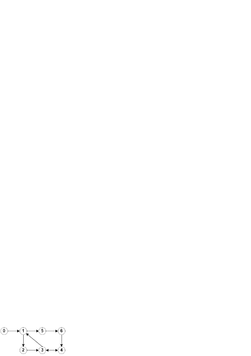
for $i=1,\cdots,6$ . In the equations, $\theta_{ji}$ , $j=1,\cdots,6$ , $i=1,\cdots,6$ , represent unknown parameters. The leader system is given by (2) with $S=\left[\begin{array}[]{ccc}0&1\\ -1&0\\ \end{array}\right]$ and $E=I_{2}$ . The information flow among all the subsystems and the leader is described by the digraph in Fig. 1, which contains a spanning tree with node 0 as the root, satisfying Assumption II.1. Let $D=8I_{6}$ . Then $DH+H^{T}D\geq 2I_{N}$ .

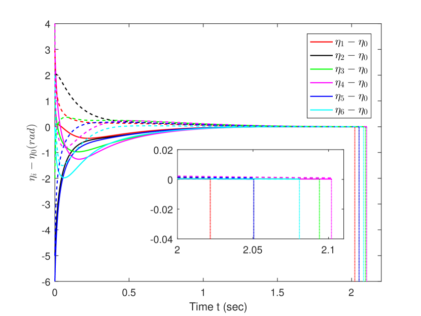
Refer to caption — Figure 1: Illustration of the communication network topology.

By Lemma III.1, let $c_{1}=8.4,~{}c_{2}=1,~{}c_{3}=1,~{}a=3/5,~{}b=3$ . Now we can construct the fixed-time observer (III) whose performance is shown in Fig. 2. It is observed that the estimation errors $\eta_{i}-\eta_{0}$ , $i=1,\cdots,6$ , approach zero at the time instants marked by the vertical lines. In the simulation, the error tolerance of numerical calculation is set as $10^{-3}$ that is used as the criterion of approaching zero.

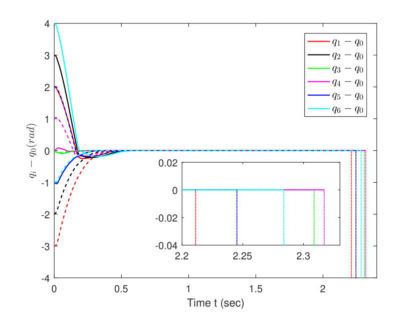
Next, we apply the observer (III) to solve the fixed-time control problem of Euler-Lagrange systems and design the fixed-time control law $\tau_{i}=\hat{M}(u_{1i}+u_{2i})$ where $u_{1i}$ is given by (21) and $u_{2i}$ is given by (25). Although we we do not know the exact value of $M_{i}(q_{i})$ , $C_{i}(q_{i},\dot{q}_{i})$ and $G_{i}(q_{i})$ , it is assumed that the unknown parameters in the following ranges $\theta_{1i}\in[6,8]$ , $\theta_{2i}\in[0.8,1]$ , $\theta_{3i}\in[1,1.4]$ , $\theta_{5i}\in[1.5,2]$ , and $\theta_{6i}\in[1,1.3]$ . Simple calculation verifies that the properties in (15) are satisfied for $k_{\underline{m}}^{-1}=0.3,~{}k_{\overline{m}}^{-1}=0.08,~{}k_{c}=3$ , and $k_{g}=50$ . We select the parameters in (21) and (25) as $\kappa=3,~{}\epsilon=11/19,~{}\gamma_{1}=10,~{}\gamma_{2}=10,~{}k_{1}=20,~{}k_{2}=15,~{}\alpha={7}/{9},~{}\beta={9}/{7}$ . For the purpose of simulation, we provide the values for uncertain parameters $\theta_{1i}=7,~{}\theta_{2i}=0.96,~{}\theta_{3i}=1.2,~{}\theta_{4i}=5.96,~{}\theta_{5i}=2$ , and $\theta_{6i}=1.2$ . The simulation is conducted with arbitrarily selected initial conditions. 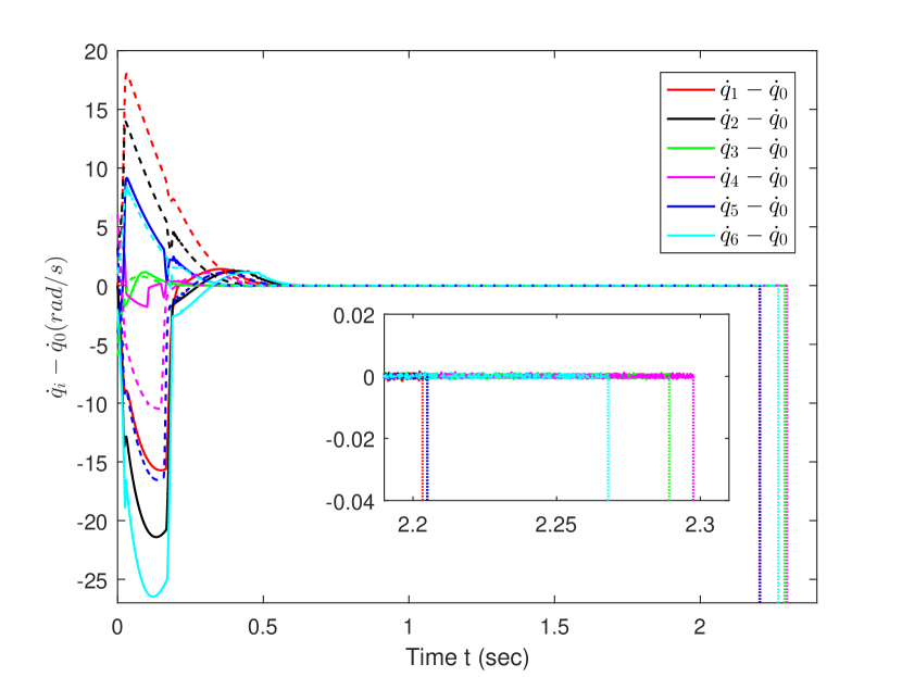Fig. 3 shows $q_{i}$ , $\dot{q}_{i}$ respectively converge to $q_{0}$ , $\dot{q}_{0}$ in fixed time instants.

VI Conclusion

This paper has proposed the fixed-time robust control design for the consensus problem of networked Euler-Lagrange systems based on a distributed observer, which is capable of estimating the desired trajectory of the leader in a fixed time under a directed graph. The heterogeneous uncertain Euler-Lagrange systems are converted into second-order systems by a partial design of the control law, and then the backstepping procedure for second-order systems are utilized to accomplished the fixed-time control design.

References

[1] S. P. Bhat and D. S. Bernstein, “Continuous finite-time stabilization of the translational and rotational double integrators,” IEEE Transactions on Automatic Control, vol. 43, no. 5, pp. 678–682, 1998.
[2] F. Xiao, L. Wang, J. Chen, and Y. Gao, “Finite-time formation control for multi-agent systems,” Automatica, vol. 45, no. 11, pp. 2605–2611, 2009.
[3] J. Fu and J. Wang, “Observer-based finite-time coordinated tracking for general linear multi-agent systems,” Automatica, vol. 66, pp. 231–237, 2016.
[4] Y. Cao and W. Ren, “Finite-time consensus for multi-agent networks with unknown inherent nonlinear dynamics,” Automatica, vol. 50, no. 10, pp. 2648–2656, 2014.
[5] H. Du, G. Wen, D. Wu, Y. Cheng, and J. Lü, “Distributed fixed-time consensus for nonlinear heterogeneous multi-agent systems,” Automatica, vol. 113, p. 108797, 2020.
[6] Z. Zuo, “Nonsingular fixed-time consensus tracking for second-order multi-agent networks,” Automatica, vol. 54, pp. 305–309, 2015.
[7] Z. Zuo, B. Tian, M. Defoort, and Z. Ding, “Fixed-time consensus tracking for multiagent systems with high-order integrator dynamics,” IEEE Transactions on Automatic Control, vol. 63, no. 2, pp. 563–570, 2018.
[8] Y. Hong, Y. Xu, and J. Huang, “Finite-time control for robot manipulators,” Systems & Control Letters, vol. 46, no. 4, pp. 243–253, 2002.
[9] Y. Hong, J. Wang, and D. Cheng, “Adaptive finite-time control of nonlinear systems with parametric uncertainty,” IEEE Transactions on Automatic Control, vol. 51, no. 5, pp. 858–862, 2006.
[10] X. Huang, W. Lin, and B. Yang, “Global finite-time stabilization of a class of uncertain nonlinear systems,” Automatica, vol. 41, pp. 881–888, 2005.
[11] S. Yu, X. Yu, B. Shirinzadeh, and Z. Man, “Continuous finite-time control for robotic manipulators with terminal sliding mode,” Automatica, vol. 41, no. 11, pp. 1957–1964, 2005.
[12] D. Zhao, S. Li, and F. Gao, “A new terminal sliding mode control for robotic manipulators,” International Journal of control, vol. 82, no. 10, pp. 1804–1813, 2009.
[13] M. Galicki, “Finite-time control of robotic manipulators,” Automatica, vol. 51, pp. 49–54, 2015.
[14] J. Huang, C. Wen, W. Wang, and Y.-D. Song, “Adaptive finite-time consensus control of a group of uncertain nonlinear mechanical systems,” Automatica, vol. 51, pp. 292–301, 2015.
[15] H.-X. Hu, G. Wen, W. Yu, J. Cao, and T. Huang, “Finite-time coordination behavior of multiple Euler–Lagrange systems in cooperation-competition networks,” IEEE transactions on cybernetics, vol. 49, no. 8, pp. 2967–2979, 2019.
[16] A. Polyakov, “Nonlinear feedback design for fixed-time stabilization of linear control systems,” IEEE Transactions on Automatic Control, vol. 57, no. 8, pp. 2106–2110, 2012.
[17] Y. Su, “Cooperative global output regulation of second-order nonlinear multi-agent systems with unknown control direction,” IEEE Transactions on Automatic Control, vol. 60, no. 12, pp. 3275–3280, 2015.
[18] R. A. Horn, R. A. Horn, and C. R. Johnson, Topics in Matrix Analysis. Cambridge University Press, 1994.
[19] G. H. Hardy, J. E. Littlewood, and G. Pólya, Inequalities. Cambridge University Press, 1952.
[20] C. Qian and W. Lin, “A continuous feedback approach to global strong stabilization of nonlinear systems,” IEEE Transactions on Automatic Control, vol. 46, no. 7, pp. 1061–1079, 2001.
[21] Y. Song, Y. Wang, J. Holloway, and M. Krstic, “Time-varying feedback for regulation of normal-form nonlinear systems in prescribed finite time,” Automatica, vol. 83, pp. 243–251, 2017.

	$\displaystyle\\|Y_{i}\\|^{2}=$	$\displaystyle\\|c_{1}y_{i}+c_{2}\mbox{sig}^{a}(y_{i})+c_{3}\mbox{sig}^{b}(y_{i}))\\|^{2}$
	$\displaystyle\geq$	$\displaystyle c_{1}^{2}\\|y_{i}\\|^{2}+c_{2}^{2}\\|\mbox{sig}^{a}(y_{i})\\|^{2}+c_{3}^{2}\\|\mbox{sig}^{b}(y_{i})\\|^{2}$
	$\displaystyle\geq$	$\displaystyle c_{1}^{2}\\|y_{i}\\|^{2}+c_{2}^{2}\\|y_{i}^{2a}\\|_{1}+c_{3}^{2}\\|y_{i}^{2b}\\|_{1}.$

	$\displaystyle V^{\frac{2a}{1+a}}\leq$	$\displaystyle\sum_{i=1}^{N}\Big{(}(\frac{c_{1}d_{i}}{2})^{\frac{2a}{1+a}}\\|y_{i}^{\frac{4a}{1+a}}\\|_{1}+(\frac{c_{2}d_{i}}{1+a})^{\frac{2a}{1+a}}\\|y_{i}^{2a}\\|_{1}$
		$\displaystyle+(\frac{c_{3}d_{i}}{1+b})^{\frac{2a}{1+a}}\\|y_{i}^{\frac{2a(1+b)}{1+a}}\\|_{1}\Big{)}$
	$\displaystyle\leq$	$\displaystyle\hat{c}_{2}\left((\\|y\\|^{2})^{\frac{2a}{1+a}}+(\\|y\\|^{2})^{a}+(\\|y\\|^{2})^{\frac{a(1+b)}{1+a}}\right)$

	$\displaystyle(\\|y\\|^{2})^{\frac{2a}{1+a}}\leq$	$\displaystyle\\|y\\|^{2}+(\\|y\\|^{2})^{a}$
	$\displaystyle(\\|y\\|^{2})^{\frac{a(1+b)}{1+a}}\leq$	$\displaystyle(\\|y\\|^{2})^{a}+(\\|y\\|^{2})^{b}$

	$\displaystyle(\\|y\\|^{2})^{\frac{2b}{1+b}}\leq$	$\displaystyle\\|y\\|^{2}+(\\|y\\|^{2})^{b}$
	$\displaystyle(\\|y\\|^{2})^{\frac{b(1+a)}{1+b}}\leq$	$\displaystyle(\\|y\\|^{2})^{a}+(\\|y\\|^{2})^{b}$

	$\displaystyle\\|M_{i}^{-1}(q_{i})\hat{M}-I_{m}\\|=$	$\displaystyle\\|\frac{2M_{i}^{-1}}{k_{\underline{m}}^{-1}+k_{\overline{m}}^{-1}}-I_{m}\\|\leq\epsilon$
	$\displaystyle\\|F_{i}(q_{i},v_{i})\\|\leq$	$\displaystyle k_{\underline{m}}^{-1}(k_{c}\\|v_{i}\\|^{2}+k_{g})=f_{i}(v_{i}),$