Flavor Constraints in a Generational Three Higgs Doublet Model
Abstract
We propose a Three Higgs Doublet Model (3HDM) that goes beyond natural flavor conservation and in which each of the three Higgs doublets couples mainly to a single generation of fermions via non-standard Yukawa structures. A hierarchy in the vacuum expectation values of the three Higgs doublets can partially address the SM flavor puzzle. In light of the experimentally observed GeV Higgs boson, we primarily work within a 3HDM alignment limit such that a Standard Model-like Higgs is recovered. In order to reproduce the observed CKM mixing among quarks, the neutral Higgs bosons of the theory necessarily mediate flavor changing neutral currents at the tree level. We consider constraints from neutral kaon, meson, and meson mixing as well as from the rare leptonic decays . We identify regions of parameter space in which the new physics Higgs bosons can be as light as a TeV or even lighter.
I Introduction
Measurements of Higgs properties at the LHC [1, 2] indicate that the Higgs is to good approximation Standard Model (SM) like. This is particularly the case for its couplings to gauge bosons and third generation fermions. However, little is still known about the small Higgs couplings to the first and second generation fermions. While evidence for the decay of the Higgs into muons has been established [3, 4], there is still large room for new physics in all its couplings to the first and second generation.
In this context, it is interesting to speculate that not all fermion masses originate from a single source of electroweak symmetry breaking but that the light fermions might obtain their masses from a second, subdominant source. Setups along this line have been proposed e.g. in [5, 6, 7, 8, 9, 10]. Part of the motivation of such scenarios is related to aspects of the SM flavor puzzle [11], i.e. the question of why the observed masses of quarks and leptons and the quark mixing exhibit a very hierarchical pattern. The first and second generation of quarks and leptons might be much lighter than the third generation because their masses are proportional to a much smaller source of electroweak symmetry breaking.
This idea has been implemented in the “flavorful” Two Higgs doublet model (2HDM) [12, 13, 14, 15]. One Higgs couples with approximately SM-like interactions to gauge bosons and the third generation fermions, while a second Higgs provides masses for the first and second generation. A mass hierarchy between the third generation and the first two generation can be explained by a hierarchy in vacuum expectation values of the two Higgs bosons. In this work we explore if this idea can be extended to all three generations in the context of a Three Higgs doublet model (3HDM). We are interested in a “generational” 3HDM, with each of the three Higgs bosons coupling to a single generation of fermions through rank-1 Yukawa matrices. The observed hierarchy between the masses of the three generations (or part of this hierarchy) may then be explained by a hierarchical pattern of the three Higgs vacuum expectation values.
A vast literature exists on the topic of 3HDMs, with many studies appearing within the past decade. Aspects of 3HDMs (or in general models with more than two Higgs doublets) that are extensively discussed include the structure of the scalar potential [16, 17, 18, 19, 20, 21, 22, 23, 24, 25, 26, 27, 28, 29, 30, 31, 32, 33, 34, 35, 36, 37, 38, 39], the presence of new sources of CP violation and applications to baryogenesis or leptogenesis [40, 41, 42, 43, 44, 45], the possible presence of a dark matter candidate if at least one the doublets is inert [46, 47, 48, 49, 50, 51, 52], interesting collider phenomenology of the additional Higgs bosons [53, 54, 55, 56, 57, 58, 59], as well as other phenomenological implications [60, 61, 62, 63, 64].
The most relevant aspect for our work is the flavor phenomenology of 3HDMs (see e.g. [65, 66, 67, 68, 69, 70, 71, 72, 73, 74]). As we will see, in order to reproduce the observed mixing in the quark sector, our model necessarily violates the principle of natural flavor conservation [75] and therefore features flavor changing neutral currents already at the tree level. The main goal of our paper is to consistently set up the model and to identify the most important flavor constraints. We find that the most generic version of our 3HDM gives large contributions to meson mixing, kaon mixing in particular, from the tree level exchange of neutral Higgs bosons. In such a region of parameter space, the meson mixing constraints push the additional Higgs bosons to scales that are not collider accessible. However, if only the minimal amount of flavor violation required to reproduce the CKM matrix is present, flavor constraints are much more relaxed. In that case, we find that the strongest constraints come from leptonic decays of mesons and kaons, and Higgs masses around 1-2 TeV are not excluded. An exploration of the distinct collider phenomenology of such a setup is left for future work.
This paper is structured as follows: In section II, we introduce the generational 3HDM. We discuss in detail the scalar sector, including electroweak symmetry breaking, the physical Higgs spectrum, as well as approximations that are valid in the limit of hierarchical vacuum expectation values. We also spell out our assumptions about the Yukawa sector and determine the couplings of the physical Higgs bosons with quarks and charged leptons. In section III, we discuss the most relevant low-energy flavor constraints of our model. We cover neutral meson mixing and rare leptonic decays of mesons and kaons, , , and . We conclude and summarize our results in section IV. Details about renormalization group running for meson mixing constraints and a simple setup that generates rank-1 Yukawa couplings are presented in appendices A and B, respectively.
II A generational three Higgs doublet model
II.1 The field content and the Lagrangian
We augment the SM with two additional Higgs doublets. The associated gauge representations under are analogous to the SM. All three Higgs doublets transform as , with labeling the three Higgs fields.
The terms in the model’s Lagrangian that contain the Higgs fields can be written as
| (1) |
In addition to the kinetic terms, the Lagrangian contains a potential for the Higgs fields and Yukawa interactions with the SM fermions. The most general Yukawa Lagrangian is
| (2) |
where and are flavor indices which run from 1 to 3. and represent the left-handed quark and lepton doublets, while , , are the quark and lepton singlets. The matrices denote the Yukawa couplings. Neutrino masses and mixing are beyond the scope of this paper.
The most general gauge invariant HDM potential may contain up to mass parameters and quartic interactions (see e.g. [28, 33])
| (3) |
where and, by hermiticity, while . In a 3HDM, this corresponds in general to 54 terms in the Higgs potential.
As discussed in more detail in section II.4 and appendix B, we are interested in a scenario in which the three Higgs fields couple preferentially to a single generation. This can be most readily achieved if the Higgs fields are charged under softly broken flavor symmetries. We thus consider it plausible that the Higgs potential respects to a good approximation a softly broken symmetry, with the three factors acting separately on a single Higgs field. This reduces significantly the possible 54 potential terms. Explicitly, we are left with111This setup is sometimes referred to as the symmetric 3HDM in the literature, see e.g. [32]. In fact, the third is automatically guaranteed by hypercharge gauge invariance.
| (4) |
The three diagonal mass parameters as well as all nine quartic interactions of the potential are real. The three off-diagonal mass parameters, with , softly break the symmetry. They can be complex and give rise to CP violation. Note that one can in principle use the freedom to re-phase the Higgs fields and remove the imaginary parts of two of the off-diagonal mass parameters, leaving a single physical CP violating phase.
II.2 Electroweak symmetry breaking and the Higgs spectrum
We assume that the three Higgs fields acquire vacuum expectation values such that spontaneous symmetry breaking (SSB) occurs: . In particular, we assume that the vacuum expectation values (vevs) of the Higgs fields are aligned such that remains unbroken.
Based on the study of bounded from below constraints in 3HDMs that include charged runaway directions (see e.g. [32, 39]) and the study of electroweak symmetry breaking in multi-Higgs doublet models (see e.g. [17, 23]), we expect that an order 1 amount of parameter space does not break , as is common in the 3HDM literature.
In this case, we can parameterize the scalar doublets in terms of charged and neutral components in the usual way
| (5) |
The three vevs can, in principle, be complex. We find it convenient to work in a phase convention in which all three vevs are real. Without loss of generality, we label the Higgs fields such that . As discussed below in section II.4, we will construct the Yukawa sector such that the doublets , , and provide mass mainly to the first, second, and third generation of fermions, respectively. The ordering of the three vevs thus follows the mass ordering of the three generations of fermions, and we will later focus mainly on the limit , which partially addresses the hierarchies in the fermion spectrum of the SM.
In order to reproduce the masses of the and bosons, the individual vevs must sum in quadrature to the SM Higgs vev
| (6) |
This condition is satisfied by construction if we work with the convenient parameterization
| (7) |
where we used the notation , and . The above definitions imply
| (8) |
which may be viewed as an extension of the 2HDM definition for . In effect, we may trade , , for , , .
Working with real vevs implies in general that , , and all have imaginary parts. We find that these imaginary parts are related by the minimization conditions of the potential in the following way
| (9) |
The remaining minimization conditions allow us to express the mass parameters , , and in terms of the real vacuum expectation values
| (10) | ||||
| (11) | ||||
| (12) |
In what follows, we will make the simplifying assumption that the Higgs potential respects CP invariance and set . The general case with CP violation in the Higgs potential and the possible implications will be discussed elsewhere.
In the absence of CP violation, HDM models will contain physical neutral CP-even Higgs bosons, physical neutral CP-odd Higgs bosons, and physical charged Higgs bosons. The remaining CP-odd and charged degrees of freedom are Goldstone bosons () that provide the longitudinal components of the and bosons of the SM. In our 3HDM case, after SSB, we expect a total of 3 neutral CP-even Higgs bosons (, , ), 2 neutral CP-odd Higgs (, ), and 2 pairs of charged Higgs bosons (, ).
The mass matrix of the CP-odd scalars is independent of the quartic interactions and given by
| (13) |
For the charged and CP-even scalar mass matrices, we find
| (14) | |||||
| (15) |
We rotate into the physical Higgs mass-eigenstate basis through orthogonal, 3-parameter rotations for each of the three Higgs sectors
| (16) |
The diagonalization matrices , , and can be parameterized as products of three rotation matrices. We find for the pseudoscalar and charged Higgs sectors
| (17) |
| (18) |
where and where already introduced in (7). After applying the and rotations, one obtains partially diagonalized forms of the respective mass matrices, with the massless Goldstone bosons and already appearing as eigenstates. The final rotations by the angels and fully diagonalize the mass matrices and define the massive eigenstates , and , .
The pseudoscalar masses , and the mixing angle are determined by
| (19) | |||||
| (20) | |||||
| (21) |
These relations can be used to trade the Lagrangian parameters , , for , , . The charged Higgs masses , and the corresponding mixing angle can be determined analogously. We find
| (22) | |||||
| (23) | |||||
| (24) |
In the case of the CP-even Higgs bosons, we write
| (25) |
with all three angles , , and , as new parameters. As already anticipated in the introduction, the stringent limits from meson mixing generically suggest that the BSM Higgs bosons may be considerably heavier than the electroweak scale. It is thus motivated to consider the decoupling limit in which . In this limit, one finds to first approximation
| (26) |
The eigenstate has a mass of the order of and has at leading order precisely SM-like couplings. It is thus identified with the 125 GeV Higgs. As we will see in section III, in the approximation (26), an exact cancellation of new physics contributions to the meson mixing amplitudes can occur. To assess the constraints from meson mixing, it thus becomes important to systematically include corrections beyond the leading order of the decoupling limit.
II.3 Beyond the leading order of the decoupling limit with large and
While it is possible to systematically expand the masses and mixing angles in the CP even scalar sector in powers of , the resulting expressions are rather lengthy and will not be presented here. Instead, we will focus on the scenario of large and in which the expressions simplify considerably. In fact, one motivation to consider the generational 3HDM model is the possibility of partially addressing the hierarchies in the SM fermion masses. We thus consider a scenario with , corresponding to .
First of all, assuming no particular hierarchy in the mass parameters , we find that the pseudoscalar is parametrically heavier than 222According to the minimization conditions in eqs. (10) - (12), this corresponds to a hierarchical set of diagonal masses . Alternatively, one could entertain a scenario with , which gives , but requires . In our numerical analysis, we do not assume any particular hierarchy in the masses of the heavy Higgs bosons.
| (27) |
Moreover, the mixing angle in the pseudoscalar sector, , turns out to be small and is of the order of . More precisely, we find
| (28) |
In the charged Higgs sector, the masses and mixing angles are given at leading order by the corresponding pseudoscalar quantities. Including next-to-leading order corrections, we find
| (29) |
Similarly, for the masses of the scalar Higgs bosons we find
| (30) | |||||
| (31) |
For the diagonalization matrix in the scalar Higgs sector, we find it convenient to write
| (32) |
where the matrix captures the departure from the decoupling limit. We find
| (33) | |||||
| (34) | |||||
| (35) |
II.4 The Yukawa sector
We consider the following set of Yukawa matrices, with textures that are an extension of the textures previously explored in the context of so-called flavorful 2HDMs [13, 12, 14]
| (36a) | ||||||||
| (36b) | ||||||||
| (36c) | ||||||||
With we indicate the order of the entries, keeping in mind that non-zero entries in the same matrix can differ by complex factors. We assume that all of the Yukawa couplings are rank-1 matrices, but otherwise do not contain any specific structure. Because of the assumed rank-1 structure, each Higgs doublet couples only to a single linear combination of the three generations and we dub such a scenario a “generational” 3HDM (or G3HDM). The rank-1 structure of the Yukawas can be realized in a straight-forward way by having the SM fermions mix with three separate generations of vector-like fermions that each couple to only one of the Higgs doublets. More details are given in appendix B.
An interesting feature of the generational 3HDM setup is that one may choose to generate part of the SM fermion mass hierarchies by adjusting the vevs of the three doublets relative to each other. This offers the option to either generate the large mass differences purely in the Yukawa sector, as seen in the SM, or to shift some of the burden over to the Higgs sector. In the limit of a large relative vev hierarchy, , one may begin with a set of rank-1 and Yukawa couplings, and proceed to have the large parts of the quark and lepton mass hierarchies be generated in the Higgs sector alone.
Without loss of generality, we have expressed the Yukawa couplings in a flavor basis in which the couplings of are diagonal, emphasizing the role of in providing the dominant component of the mass for the third generation of quarks and leptons. Note that the couplings of preserve a flavor symmetry that acts on the first two generations. The couplings of and are in general misaligned in flavor space and both break the symmetry. However, we can use the remaining freedom in choosing a flavor basis to bring the couplings of into the shown block-diagonal form.
The non-minimal breaking of the SM flavor symmetries by the above set of Yukawa couplings is expected to give large contributions to flavor-changing neutral current (FCNC) processes, kaon and meson mixing in particular. The corresponding flavor constraints on the model will be analyzed in detail in section III. In order to soften the constraints one may entertain the possibility that some of the off-diagonal entries in and are suppressed compared to what is shown in (36a) - (36c). This could for example be achieved by spontaneously broken flavor symmetries. However, we emphasize that not all off-diagonal entries in the Yukawa couplings can be arbitrarily suppressed. The entries in and of order , , and , where is the sine of the Cabibbo angle, are required to reproduce the CKM matrix, once one rotates in the fermion mass eigenstate basis. Note that it is an assumption that the CKM matrix originates from the diagonalization of the down-quark mass matrix. Other Yukawa textures can also be viable (see also footnote 3 below.)
In the fermion mass eigenstate basis, we define the following set of mass parameters which we will use below to write the couplings of the physical Higgs mass eigenstates to fermion mass eigenstates
| (37) |
These parameters obey the relationship
| (38) |
with (without superscripts) representing the physical masses of the quarks or leptons.
We obtain the following set of explicit mass parameters after expanding each entry to leading order in ratios of first to second and second to third generation masses
| (39) |
| (40) |
| (41) |
| (42) |
The lepton mass parameters are completely analogous to the ones in the up quark sector. In the above expressions, the , are free, in general complex, parameters. These parameterize new sources of flavor and CP violation. Note that not all entries of the mass matrices are independent. This is due to two reasons: first, they need to reproduce the quark and lepton masses as well as the CKM matrix; second, we have assumed that they originate from rank-1 Yukawa couplings.
It is in principle possible to set all the , to zero. In that case, one obtains a “generation specific” 3HDM in which the Yukawa couplings are aligned such that , , and couple to a good approximation only to the first, second, and third generation, respectively. The alignment can be exact in the up-quark sector and the lepton sector. However, because in the described setup the CKM matrix originates from the down Yukawa couplings, the alignment cannot be perfect in the down sector. The mass matrices , , contain necessarily also flavor changing entries333Alternatively, the CKM matrix could be generated in the up-sector. In that case one could have an exact alignment in the down quark sector, but the up quark mass matrices , , would contain off-diagonal terms. In the most generic case, the CKM matrix would originate partly from the down-sector and partly from the up-sector. .
II.5 Couplings of the physical Higgs bosons
After bringing both fermions and scalars into the mass eigenstate basis, the couplings of the physical Higgs bosons of the 3HDM to the SM fermions may be parameterized by
| (43) |
We introduced the modifiers that parameterize the deviation from the related SM couplings. In the SM, for the diagonal Higgs couplings, whereas for the off-diagonal couplings. It is straight-forward to express the factors in terms of mass parameters in (39) - (42) and the mixing angles in the Higgs sector defined in (17), (18), and (25),
| (44) |
As the resulting explicit expressions are very lengthy, we refrain from showing them here. Instead, we give approximate expressions that are valid in the combined limit and . We find for the CP-odd Higgs couplings
| (45) | |||||
| (46) |
The factors of the CP even Higgs bosons are tightly related to the ones of the CP odd Higgs bosons. For all types of fermions one has
| (47) | |||||
| (48) | |||||
| (49) |
Finally, for the charged Higgs bosons we find
| (50) |
III Low Energy Flavor Probes
As seen in the previous section, the Higgs bosons of the considered setup in general all have flavor-changing couplings. One thus expects that flavor-changing neutral current (FCNC) processes can be used to constrain the model. This is particularly the case for neutral meson mixing and rare leptonic decays of neutral mesons, which all receive tree-level contributions from neutral Higgs boson exchange. As detailed below, we indeed find that observables related to the mentioned FCNC processes provide often stringent constraints on our Higgs parameter space as many of the observables have been measured to a high accuracy and there exist robust SM predictions for most cases considered.
III.1 Meson oscillations
The frequencies of neutral kaon and meson oscillations are measured with impressive accuracy [76, 77, 78, 79]. Also the parameter that measures indirect CP violation in kaon oscillations is known experimentally with high precision [78], as are the and mixing phases [79, 80, 81]. The experimental status is summarized in the left column of Table 1.
| observable | experiment | SM prediction (from tree level CKM) |
|---|---|---|
| [78] | [82] | |
| [79] | ||
| [79] | ||
| [78] | ||
| [79, 80] | ||
| [79, 81] |
The SM predictions we use are collected in the right column of Table 1. For the neutral kaon oscillation frequency , we quote the short-distance contribution [82]. Keeping in mind that there are also long-distance contributions that are poorly controlled so far [83, 84], we use in our numerical analysis . We obtain the SM predictions of the remaining observables following [85]. Among the most relevant input parameters are CKM matrix elements that we determine from the PDG values [78]
| (51) |
The values for and are conservative averages of determinations using inclusive and exclusive tree level decays. For the sine of the Cabibbo angle, we use [78], neglecting its tiny uncertainty. The hadronic matrix elements needed for the SM predictions of and are taken from [86]. Overall, there is very good agreement between the measurements and the corresponding SM predictions. In most cases, the size of possible new physics contributions is limited by the precision of the SM predictions.
The relevant observables in the neutral meson systems are the mass differences and mixing phases that can be calculated from the new physics contributions to the mixing amplitudes, which we denote by
| (52) |
Similarly, the relevant observables for kaon mixing are the mass difference and the CP violating parameter , and they can be expressed as
| (53) |
where [78].
In the considered 3HDM setup, the dominant new physics contributions arise from the tree-level exchange of the neutral Higgs bosons. The expressions for and mixing are an extension of the flavorful 2HDM expressions [14], and we find
| (54) |
where is a SM loop function. The parameters , , and encapsulate 1-loop QCD renormalization group running and ratios of hadronic matrix elements. Setting the renormalization scale to TeV and using hadronic matrix elements from [87], we find
| (55) | |||
| (56) |
for mixing and for mixing, respectively. Natural choices for the renormalization scale are the masses of the neutral Higgs bosons. The values of the depend logarithmically on the scale and stay within when varying it between GeV and TeV. Explicit expressions for the factors are provided in appendix A.
The final ingredient to evaluate eq. (54) are the quark mass ratios . The ratios are to a very good approximation RGE invariant, and we use [78, 88, 89]
| (57) |
In the phenomenologically interesting limit there is an approximate cancellation in the terms in the second line of eq. (54). In this case, using the expressions for the factors from section II, we find
| (58) | |||||
| (59) |
Based on the above expressions and using the values collected in Table 1, we can derive simple analytical bounds on and . Assuming that there are no accidental cancellations, setting the absolute values of the and parameters to 1, and marginalizing over their phases, we find
| (60) | ||||
| (61) |
For moderately large values of and , we find that the masses of the additional Higgs bosons get pushed into the multi-TeV range.
In the scenario in which all , the expressions in eqs. (58) and (59) vanish, and one needs to expand one order higher in to find the leading contribution. An analogous behavior was observed in the context of flavorful 2HDMs [14] and is a well-known phenomenon in 2HDMs in general [90]. Making use of the results in section II.3, we find
| (62) | |||||
| (63) |
Interestingly, in this case, the expressions are independent of and , and one can directly obtain bounds on the masses and . Assuming the absence of accidental cancellations and assuming that the relevant combinations of quartic coupling are 1, we find
| (64) | |||||
| (65) |
We do not obtain a meaningful bound on from mixing. The bounds that can be obtained are rather weak, of the order of the electroweak scale. Given our approximations, we expect uncertainties on those bounds.
Moving on to kaon oscillations, the new physics contributions to the mixing amplitude can be generically written as
| (66) |
For the kaon decay constant and the hadronic bag parameters we use MeV [91] and , , [92]. The factors correspond to corrections from the 1-loop QCD renormalization group running from the high new physics scale to the low scale at which the kaon matrix elements are evaluated. For a new physics scale of TeV we find
| (67) |
Explicit expressions for the factors are given in appendix A.
In the decoupling limit , the expression simplifies considerably
| (68) |
Setting the absolute value of the parameter to 1 and marginalizing over its phase, we find the following bounds on the Higgs masses
| (69) |
In the generic case, we see that the additional Higgs bosons are far outside the reach of the LHC, even for moderate values of and .
If we profile over the phase of instead of marginalizing over it, the situation is qualitatively different, as the strong constraint from is avoided and only the much weaker constraint from applies. In this approach, we find
| (70) |
If the parameter is set to 0, the leading contribution to the kaon mixing amplitude is given by
| (71) |
If the quartic couplings are assumed to be and barring accidental cancellations, we find
| (72) |
These constraints are fairly weak and in the same ballpark as the numbers we found from and mixing when the and were switched off.
For completeness, we also discuss the constraints from neutral meson mixing. The expressions for the mixing amplitude are very similar to the case of kaon mixing, with the obvious replacements of couplings, masses, and hadronic parameters
| (73) |
The parameters have already been introduced in eq. (67). The meson decay constant, and the bag parameters are MeV [91] and , , [92]. For the ratio of up to charm quark mass, we use [78, 88, 89]
| (74) |
In the decoupling limit, the expression for the mixing amplitude simplifies to
| (75) |
On the experimental side, neutral meson mixing is firmly established [79]. Assuming no direct CP violation in doubly Cabibbo suppressed meson decays (which is an excellent approximation in our setup), HFLAV directly provides constraints on the mixing amplitude parameterized by , with the neutral meson lifetime s, and the CP violating phase . We find that the confidence regions in the plane shown by HFLAV [79] can be reproduced with high accuracy by
| (76) |
The SM prediction for the mixing amplitude is expected to be real to a good approximation, but its size is not well known (see e.g. [93] for a review). In our numerical analysis, we allow the SM contribution to saturate the experimental central value of the real part with 100% uncertainty
| (77) |
To find bounds on the Higgs masses, we set the absolute value of the parameter combination , which enters the new physics contribution to the mixing amplitude, to 1 and marginalizing over its phase. We find
| (78) |
This is considerably weaker than the corresponding constraint from kaon mixing. We do not find a meaningful bound from mixing when we profile over the new physics phase. The constraints from mixing can be avoided entirely if the parameters in the up sector are set to zero.
So far, we have seen that meson mixing generically puts very strong constraints on the model. In the presence of flavor violating parameters , with CP violating phases, the strongest constraint comes from kaon mixing, and the results above suggest that the additional Higgs bosons have to have masses of at least 10 TeV or even 100 TeV for moderately large and .
If the new flavor violating parameters are very small, , an irreducible amount of flavor mixing remains due to the CKM matrix. However, in that case, the new physics contributions to meson mixing turn out to be fairly small, and Higgs boson masses below the 1 TeV scale can be compatible with constraints from meson mixing. Therefore, it is important to consider additional flavor observables that are sensitive to the new Higgs bosons and could provide stronger constraints.
III.2 Rare meson decays and
The rare decays of neutral mesons into a charged lepton pair, and , the decay in particular, are known to be sensitive probes of extended scalar sectors [94, 95, 96].
The branching ratios of these meson decays can be predicted with very high precision. The largest uncertainty stems from the relevant CKM matrix elements. Using the results from [97, 98] and the CKM input from eq. (51) we find
| (79) | |||||
| (80) | |||||
| (81) | |||||
| (82) |
On the experimental side, is well established, while only upper bounds exist for . The world averages from the PDG are based on LHCb, CMS, and ATLAS results [99, 100, 101, 78], and read
| (83) | |||||
| (84) |
The experimental sensitivities to and are still far above the SM predictions. The strongest constraints on the branching ratios come from LHCb [102]
| (85) | |||||
| (86) |
In the presence of NP, the expression for BR may be generally written as [103, 95]
| (87) |
where the effective lifetime difference in the meson system is parameterized by [79]. In writing eq. (87), we have ignored a possible non-standard mixing phase , which is justified given the strong constraints from measurements [79, 81] (see Table 1).
The coefficients and depend on possible new physics contributions. In the SM, and , while in our 3HDM setup we find
| (88) |
| (89) |
The SM Wilson coefficient is . Analogous expressions hold also for . Note that the width difference in the system is negligibly small .
To obtain an analytic understanding of the constraints that can be obtained from these rare decays, we expand the expressions in the limit and . We also assume that the flavor-violating parameters are negligible . In that case, the irreducible contributions to are given by
| (90) |
As one can expect, the dominant contributions to come from the “second generation” Higgs bosons. The contributions from the “first generation” Higgs bosons are suppressed by a factor . Also note that is a free parameter and can in principle be made arbitrarily small. No robust constraints can therefore be obtained on .
A similar picture emerges for . For this decay, we find
| (91) |
Focusing on the “second generation” Higgs bosons, we estimate the following bounds
| (92) | |||||
| (93) |
The small low-mass window that is allowed by corresponds to a large new physics amplitude that interferes destructively with the SM and gives a SM-like branching ratio. Such a scenario is starting to be disfavored by measurements of the effective lifetime [95, 104], but not fully excluded yet by alone.
For moderate , the bounds we find from and are stronger than the ones from and mixing in eqs. (64) and (65), and their strength increases with increasing .
We checked if relevant bounds can be obtained from and . Using the same approximations as above, we find the new physics contributions
| (94) | |||||
| (95) |
III.3 Rare kaon decays
We also investigated the constraints that can be obtained from rare kaon decays. In particular, one can expect that the decay can provide relevant constraints on the “first generation” Higgs bosons. In the following, we will discuss and . The corresponding decays are not yet observed, and existing limits on their branching ratios [105, 106] have much weaker sensitivity to our scenario.
The decays receive large long-distance contributions from . Adapting the results from [107, 108, 109] we find the following expression for the branching ratios in our 3HDM scenario
| (96) |
The imaginary and real parts of the coefficient are given by
| (97) | |||||
| (98) |
where is the di-logarithm function and is the velocity of the leptons in the kaon restframe. The approximate expressions in equations (97) and (98) hold with high accuracy for electrons but not for muons.
The renormalization scale dependent function is a low energy coupling that is related to the off-shell form factor. Precise predictions have been obtained in [109], , (see also the previous evaluations in [110, 107, 108]).
The short distance contributions to the decays are encoded in the SM coefficient , and the lepton specific new physics contributions , and . Neglecting QED running effects and making use of isospin symmetry for the kaon masses and decay constants , we find
| (99) |
| (100) |
where [78] is the sine of the Cabibbo angle. The SM part, , contains the top contribution [111] and the charm contribution [112, 109]. The and branching ratios and lifetimes that enter the above expressions are , and s, s [78].
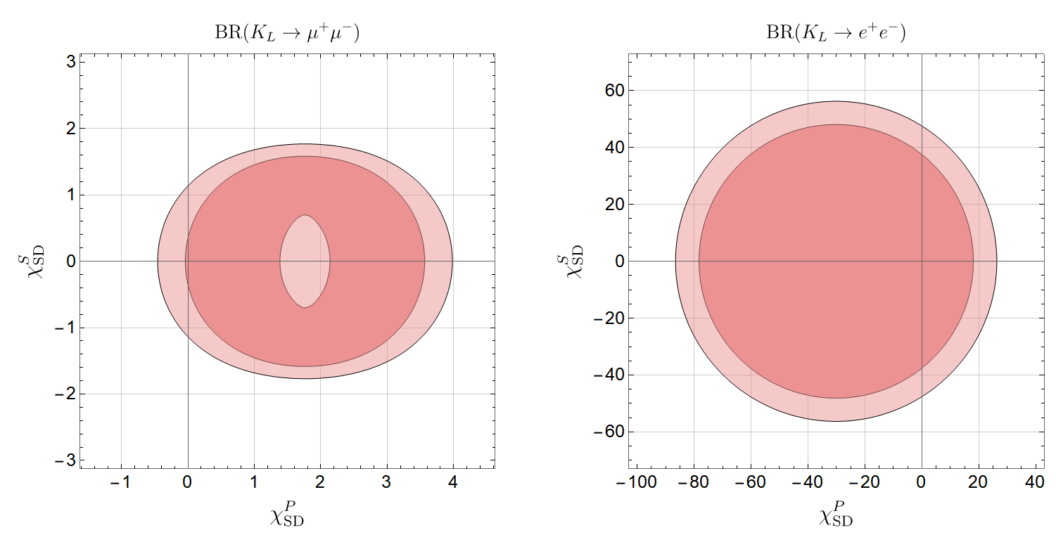
Experimentally, the decay is measured with high precision, while there is hardly evidence for the extremely rare decay. Normalizing the corresponding branching ratios to the branching ratio of the decay one has [78, 109]
| (101) | |||||
| (102) |
Based on these experimental results, we find the allowed regions in vs. parameter space shown in figure 1.
In the phenomenologically interesting limit and , and assuming that the flavor-violating parameters are negligible we find the following approximate results for the new physics parameters and for muons
| (103) | |||||
| (104) |
and for electrons
| (105) | |||||
| (106) |
As one might expect, we find relevant constraints on the second generation Higgs boson from and on the first generation Higgs boson from . The approximate bounds on the Higgs masses are
| (107) | |||||
| (108) |
The bound from is particularly strong, surpassing the one from quoted in equation (92).
III.4 Summary of the flavor constraints
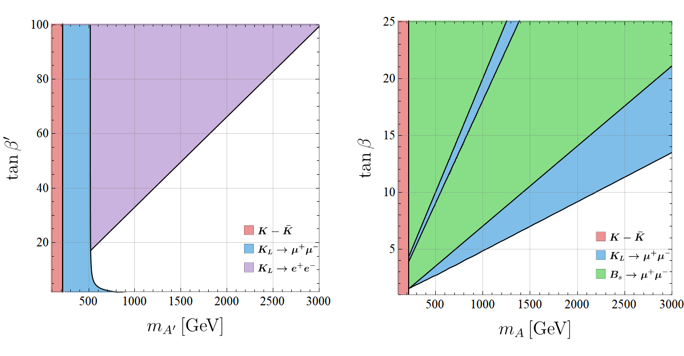
As discussed in the previous section, neutral meson mixing constraints push the masses of the additional Higgs bosons far into the multi-TeV range if the flavor parameters and are generic (i.e. if their magnitudes are of order 1). We therefore focus on the “generation-specific” limit, , which contains only the minimal amount of flavor violation to reproduce the observed quark mixing. In figure 2, we summarize the most important flavor constraints in this limit. The plot on the left shows the constraints on the “first generation” Higgs boson parameters and , while the one on the right shows the constraints on the “second generation” Higgs boson parameters and . The colored regions are excluded at the 95% C.L. by the indicated processes. Only the most stringent constraints are shown.
To obtain the bounds displayed in figure 2, we use the generation specific relationships for each process within the context of the decoupling limit (i.e. equations (103)-(106) for the leptonic decays, equations (90), (91), (94), and (95) for the leptonic and decays, and equations (62), (63), and (68) for meson mixing). The meson mixing expression automatically vanishes in the “generation specific” regime. We further fix and send the masses not being plotted to infinity. In other words, in obtaining constraints on the “first generation” parameters of and , we send and vice versa for the “second generation ” parameter space. This means that the shown bounds hold barring accidental cancellations among the contributions from different Higgs bosons.
In the generation specific limit, we find that provides the strongest bounds for the “first-generation” parameters and , whereas provides the strongest bounds for the “second-generation” parameters and , in particular for large and which is the best motivated region of parameter space. Kaon mixing is the most important constraint from meson mixing in both spaces, but is only relevant for low and . As one might expect, the strongest constraints on the first (second) generation Higgs bosons come from observables in which the majority of the fermions in the initial and final states are from the first (second) generation.
For a moderate hierarchy in the vacuum expectation values of the 3HDM, , the new Higgs boson masses can be comfortably as light as 1.5 TeV without violating flavor constraints. For smaller values of and , the Higgs bosons could be even lighter.
IV Conclusions and Outlook
In this paper, we explored a Three Higgs Doublet Model (3HDM) in which each of the three Higgs doublets primarily couples to a single generation of Standard Model fermions. One of the motivations for this scenario is its potential to partially address aspects of the SM flavor puzzle. In particular, the observed hierarchies in fermion masses could arise, at least in part, from a hierarchical pattern of Higgs vacuum expectation values, .
In the first part of the paper, we outlined the framework of our “generational 3HDM” in detail. The Yukawa sector is structured such that each Higgs doublet couples exclusively to one generation of fermions through rank-1 Yukawa matrices. A small number of free parameters governs the flavor misalignment among the three sets of up-type, down-type, and lepton Yukawa couplings. We assume that the flavor misalignment of the down-type Yukawas accounts for the observed CKM mixing in the SM quark sector, while the remaining flavor misalignment—parameterized by the coefficients and —can, in principle, be set to zero. To accommodate the observed SM-like Higgs boson, we focused on the 3HDM alignment limit, which naturally emerges in the decoupling regime, where the additional Higgs bosons are significantly heavier than the electroweak scale. The key parameters governing the properties of the additional Higgs states are their masses, and , as well as the ratios of vacuum expectation values and , which characterize the “second-generation Higgs” (unprimed) and “first-generation Higgs” (primed), respectively.
Due to the non-trivial flavor structure of the model, the new Higgs bosons generically exhibit flavor-changing couplings. In the second part of the paper, we constrained the model’s parameter space using flavor-changing neutral current processes. For generic flavor violation, where the parameters and are of order unity, we find that neutral meson mixing, particularly kaon mixing, imposes stringent constraints, pushing the new Higgs bosons well beyond the TeV scale and out of collider reach. However, in a scenario with the minimum amount of flavor violation (where the and are set to zero), the flavor constraints are significantly relaxed. In this case, the strongest bounds arise from rare leptonic decays of kaons and mesons, and Higgs bosons around the TeV scale remain viable. An interesting feature with regard to the flavor phenomenology is that the - parameter space is primarily constrained by processes involving mainly first generation fermions (e.g. ), while the - parameter space is constrained by processes involving mainly second generation fermions (e.g. or ). The most important bounds are summarized in Figure 2.
Our work motivates various follow up studies. Given that there are regions of parameter space in which the additional neutral Higgs bosons can have masses around the TeV scale, it would be interesting to explore the characteristic collider phenomenology. Based on the generational structure of the new Higgs boson couplings, one can expect that di-lepton resonance searches and di-jet resonance searches might already give relevant constraints on the model. Moreover, the flavor and collider signatures of the charged Higgs bosons warrant further investigation. The charged Higgs bosons can contribute to leptonic decays of charged mesons and might be probed by lepton flavor universality tests in [113, 114] and decays [115]. Finally, throughout much of our analysis, we have assumed that the tree-level Higgs potential respects CP invariance. It would be interesting to examine how our conclusions might change in the presence of CP violation in the Higgs sector.
Acknowledgments
We thank Aditya Gadam and Stefania Gori for useful discussions. The research of W.A. and K.T. is supported by the U.S. Department of Energy grant number DE-SC0010107.
Appendix A RGE running corrections to meson mixing
In section III.1 we discussed constraints on the Higgs bosons from meson mixing observables and included the effect of RGE running from the scale of the Higgs bosons to the scale of the mesons. In this appendix we provide the relevant RGE factors and ratios of hadronic matrix elements. We obtain the RGE factors from the 1-loop anomalous dimensions given in [116]. For meson mixing we find for the factors
| (109) |
| (110) |
| (111) |
where we used the definition of the hadronic matrix elements from [87]. The scale should be of the order of the heavy Higgs masses . The ratios of the bag parameters that enter the above expressions can be taken directly from table XV in [87].
The RGE factors that are relevant for kaon and meson mixing are given by
| (112) |
| (113) |
| (114) |
As above, the scale should be of the order of the heavy Higgs masses. The scale is the scale at which the kaon or meson bag parameters are evaluated. In our numerical analysis we use the bag parameters from [92].
Appendix B A model for the rank-1 Yukawa couplings
In this appendix we outline a simple construction that gives the rank-1 Yukawa couplings for the three Higgs doublets that we discussed in section II.4. If the three generations of SM fermions do not couple directly to the Higgs doublets but instead mix with three separate generations of vector-like fermions, rank-1 Yukawa couplings automatically arise, see e.g. [117].
We start by introducing three symmetries that act separately on the the three Higgs doublets
| (115) |
while all SM fermions remain uncharged. For each , we introduce a single generation of heavy vector-like matter, charged under the corresponding such that Yukawa couplings with a single Higgs are allowed
| (116) |
where the sum over runs over the three Higgs doublets. We assume that the symmetries are softly broken by mass mixing between the vector-like fermions and the SM fermions. After integrating out the vector-like fermions, the effective Yukawa interactions of the SM fermions take the form
| (117) | |||
| (118) | |||
| (119) |
These Yukawa interactions are outer products of two flavor vectors and thus rank-1 by construction.
As a by-product, the three symmetries also greatly reduce the number of Higgs potential terms as discussed in section II.1.
References
- [1] CMS collaboration, A portrait of the Higgs boson by the CMS experiment ten years after the discovery., Nature 607 (2022) 60 [2207.00043].
- [2] ATLAS collaboration, A detailed map of Higgs boson interactions by the ATLAS experiment ten years after the discovery, Nature 607 (2022) 52 [2207.00092].
- [3] CMS collaboration, Evidence for Higgs boson decay to a pair of muons, JHEP 01 (2021) 148 [2009.04363].
- [4] ATLAS collaboration, A search for the dimuon decay of the Standard Model Higgs boson with the ATLAS detector, Phys. Lett. B 812 (2021) 135980 [2007.07830].
- [5] W. Altmannshofer, S. Gori, A.L. Kagan, L. Silvestrini and J. Zupan, Uncovering Mass Generation Through Higgs Flavor Violation, Phys. Rev. D 93 (2016) 031301 [1507.07927].
- [6] D. Ghosh, R.S. Gupta and G. Perez, Is the Higgs Mechanism of Fermion Mass Generation a Fact? A Yukawa-less First-Two-Generation Model, Phys. Lett. B 755 (2016) 504 [1508.01501].
- [7] F.J. Botella, G.C. Branco, M.N. Rebelo and J.I. Silva-Marcos, What if the masses of the first two quark families are not generated by the standard model Higgs boson?, Phys. Rev. D 94 (2016) 115031 [1602.08011].
- [8] A.K. Das and C. Kao, A Two Higgs doublet model for the top quark, Phys. Lett. B 372 (1996) 106 [hep-ph/9511329].
- [9] A.E. Blechman, A.A. Petrov and G. Yeghiyan, The Flavor puzzle in multi-Higgs models, JHEP 11 (2010) 075 [1009.1612].
- [10] D. Egana-Ugrinovic, S. Homiller and P.R. Meade, Higgs bosons with large couplings to light quarks, Phys. Rev. D 100 (2019) 115041 [1908.11376].
- [11] W. Altmannshofer and A. Greljo, Recent Progress in Flavor Model Building, 2412.04549.
- [12] W. Altmannshofer, J. Eby, S. Gori, M. Lotito, M. Martone and D. Tuckler, Collider Signatures of Flavorful Higgs Bosons, Phys. Rev. D 94 (2016) 115032 [1610.02398].
- [13] W. Altmannshofer, S. Gori, D.J. Robinson and D. Tuckler, The Flavor-locked Flavorful Two Higgs Doublet Model, JHEP 03 (2018) 129 [1712.01847].
- [14] W. Altmannshofer and B. Maddock, Flavorful Two Higgs Doublet Models with a Twist, Phys. Rev. D 98 (2018) 075005 [1805.08659].
- [15] W. Altmannshofer, B. Maddock and D. Tuckler, Rare Top Decays as Probes of Flavorful Higgs Bosons, Phys. Rev. D 100 (2019) 015003 [1904.10956].
- [16] A. Barroso, P.M. Ferreira, R. Santos and J.P. Silva, Stability of the normal vacuum in multi-Higgs-doublet models, Phys. Rev. D 74 (2006) 085016 [hep-ph/0608282].
- [17] C.C. Nishi, The Structure of potentials with N Higgs doublets, Phys. Rev. D 76 (2007) 055013 [0706.2685].
- [18] I.P. Ivanov and C.C. Nishi, Properties of the general NHDM. I. The Orbit space, Phys. Rev. D 82 (2010) 015014 [1004.1799].
- [19] I.P. Ivanov, Properties of the general NHDM. II. Higgs potential and its symmetries, JHEP 07 (2010) 020 [1004.1802].
- [20] K. Kannike, Vacuum Stability Conditions From Copositivity Criteria, Eur. Phys. J. C 72 (2012) 2093 [1205.3781].
- [21] I.P. Ivanov and E. Vdovin, Discrete symmetries in the three-Higgs-doublet model, Phys. Rev. D 86 (2012) 095030 [1206.7108].
- [22] V. Keus, S.F. King and S. Moretti, Three-Higgs-doublet models: symmetries, potentials and Higgs boson masses, JHEP 01 (2014) 052 [1310.8253].
- [23] M. Maniatis and O. Nachtmann, Stability and symmetry breaking in the general three-Higgs-doublet model, JHEP 02 (2015) 058 [1408.6833].
- [24] I.P. Ivanov and C.C. Nishi, Symmetry breaking patterns in 3HDM, JHEP 01 (2015) 021 [1410.6139].
- [25] S. Moretti and K. Yagyu, Constraints on Parameter Space from Perturbative Unitarity in Models with Three Scalar Doublets, Phys. Rev. D 91 (2015) 055022 [1501.06544].
- [26] M. Maniatis and O. Nachtmann, Stability and symmetry breaking in the general -Higgs-doublet model, Phys. Rev. D 92 (2015) 075017 [1504.01736].
- [27] A. Pilaftsis, Symmetries for standard model alignment in multi-Higgs doublet models, Phys. Rev. D 93 (2016) 075012 [1602.02017].
- [28] M.P. Bento, H.E. Haber, J.C. Romão and J.a.P. Silva, Multi-Higgs doublet models: physical parametrization, sum rules and unitarity bounds, JHEP 11 (2017) 095 [1708.09408].
- [29] S. Pramanick and A. Raychaudhuri, Three-Higgs-doublet model under A4 symmetry implies alignment, JHEP 01 (2018) 011 [1710.04433].
- [30] I. de Medeiros Varzielas and I.P. Ivanov, Recognizing symmetries in a 3HDM in a basis-independent way, Phys. Rev. D 100 (2019) 015008 [1903.11110].
- [31] D. Das and I. Saha, Alignment limit in three Higgs-doublet models, Phys. Rev. D 100 (2019) 035021 [1904.03970].
- [32] F.S. Faro and I.P. Ivanov, Boundedness from below in the three-Higgs-doublet model, Phys. Rev. D 100 (2019) 035038 [1907.01963].
- [33] N. Darvishi and A. Pilaftsis, Classifying Accidental Symmetries in Multi-Higgs Doublet Models, Phys. Rev. D 101 (2020) 095008 [1912.00887].
- [34] I.P. Ivanov and F. Vazão, Yet another lesson on the stability conditions in multi-Higgs potentials, JHEP 11 (2020) 104 [2006.00036].
- [35] S. Carrolo, J.C. Romão, J.a.P. Silva and F. Vazão, Symmetry and decoupling in multi-Higgs boson models, Phys. Rev. D 103 (2021) 075026 [2102.11303].
- [36] N. Darvishi, M.R. Masouminia and A. Pilaftsis, Maximally symmetric three-Higgs-doublet model, Phys. Rev. D 104 (2021) 115017 [2106.03159].
- [37] J. Kalinowski, W. Kotlarski, M.N. Rebelo and I. de Medeiros Varzielas, 3HDM with (27) symmetry and its phenomenological consequences, JHEP 02 (2023) 231 [2112.12699].
- [38] M.P. Bento, J.C. Romão and J.a.P. Silva, Unitarity bounds for all symmetry-constrained 3HDMs, JHEP 08 (2022) 273 [2204.13130].
- [39] R. Boto, J.C. Romão and J.a.P. Silva, Bounded from below conditions on a class of symmetry constrained 3HDM, Phys. Rev. D 106 (2022) 115010 [2208.01068].
- [40] S. Weinberg, Gauge Theory of CP Violation, Phys. Rev. Lett. 37 (1976) 657.
- [41] A. Ahriche, G. Faisel, S.-Y. Ho, S. Nasri and J. Tandean, Effects of two inert scalar doublets on Higgs boson interactions and the electroweak phase transition, Phys. Rev. D 92 (2015) 035020 [1501.06605].
- [42] I. de Medeiros Varzielas, S.F. King, C. Luhn and T. Neder, CP-odd invariants for multi-Higgs models: applications with discrete symmetry, Phys. Rev. D 94 (2016) 056007 [1603.06942].
- [43] I.P. Ivanov, C.C. Nishi, J.a.P. Silva and A. Trautner, Basis-invariant conditions for symmetry of order four, Phys. Rev. D 99 (2019) 015039 [1810.13396].
- [44] I. Chakraborty and H. Roy, Type-I thermal leptogenesis in -symmetric three Higgs doublet model, Eur. Phys. J. C 80 (2020) 1038 [1909.07790].
- [45] H. Davoudiasl, I.M. Lewis and M. Sullivan, Multi-TeV signals of baryogenesis in a Higgs troika model, Phys. Rev. D 104 (2021) 015024 [2103.12089].
- [46] B. Grzadkowski, O.M. Ogreid and P. Osland, Natural Multi-Higgs Model with Dark Matter and CP Violation, Phys. Rev. D 80 (2009) 055013 [0904.2173].
- [47] V. Keus, S.F. King, S. Moretti and D. Sokolowska, Dark Matter with Two Inert Doublets plus One Higgs Doublet, JHEP 11 (2014) 016 [1407.7859].
- [48] A. Cordero, J. Hernandez-Sanchez, V. Keus, S.F. King, S. Moretti, D. Rojas et al., Dark Matter Signals at the LHC from a 3HDM, JHEP 05 (2018) 030 [1712.09598].
- [49] A. Cordero-Cid, J. Hernández-Sánchez, V. Keus, S. Moretti, D. Rojas and D. Sokołowska, Lepton collider indirect signatures of dark CP-violation, Eur. Phys. J. C 80 (2020) 135 [1812.00820].
- [50] A. Aranda, D. Hernández-Otero, J. Hernández-Sanchez, V. Keus, S. Moretti, D. Rojas-Ciofalo et al., Z3 symmetric inert ( 2+1 )-Higgs-doublet model, Phys. Rev. D 103 (2021) 015023 [1907.12470].
- [51] W. Khater, A. Kunčinas, O.M. Ogreid, P. Osland and M.N. Rebelo, Dark matter in three-Higgs-doublet models with S3 symmetry, JHEP 01 (2022) 120 [2108.07026].
- [52] A. Kunčinas, O.M. Ogreid, P. Osland and M.N. Rebelo, Dark matter in a CP-violating three-Higgs-doublet model with S3 symmetry, Phys. Rev. D 106 (2022) 075002 [2204.05684].
- [53] A.G. Akeroyd, S. Moretti and J. Hernandez-Sanchez, Light charged Higgs bosons decaying to charm and bottom quarks in models with two or more Higgs doublets, Phys. Rev. D 85 (2012) 115002 [1203.5769].
- [54] M. Merchand and M. Sher, Three doublet lepton-specific model, Phys. Rev. D 95 (2017) 055004 [1611.06887].
- [55] J.E. Camargo-Molina, T. Mandal, R. Pasechnik and J. Wessén, Heavy charged scalars from fusion: A generic search strategy applied to a 3HDM with family symmetry, JHEP 03 (2018) 024 [1711.03551].
- [56] A.G. Akeroyd, S. Moretti and M. Song, Light charged Higgs boson with dominant decay to quarks and its search at the LHC and future colliders, Phys. Rev. D 98 (2018) 115024 [1810.05403].
- [57] A.G. Akeroyd, S. Moretti and M. Song, Light charged Higgs boson with dominant decay to a charm quark and a bottom quark and its search at LEP2 and future colliders, Phys. Rev. D 101 (2020) 035021 [1908.00826].
- [58] M. Chakraborti, D. Das, M. Levy, S. Mukherjee and I. Saha, Prospects for light charged scalars in a three-Higgs-doublet model with Z3 symmetry, Phys. Rev. D 104 (2021) 075033 [2104.08146].
- [59] I.P. Ivanov and S.A. Obodenko, Constraining CP4 3HDM with Top Quark Decays, Universe 7 (2021) 197 [2104.11440].
- [60] W. Grimus, L. Lavoura, O.M. Ogreid and P. Osland, A Precision constraint on multi-Higgs-doublet models, J. Phys. G 35 (2008) 075001 [0711.4022].
- [61] A.G. Akeroyd, S. Moretti, K. Yagyu and E. Yildirim, Light charged Higgs boson scenario in 3-Higgs doublet models, Int. J. Mod. Phys. A 32 (2017) 1750145 [1605.05881].
- [62] M.A. Solberg, Conditions for the custodial symmetry in multi-Higgs-doublet models, JHEP 05 (2018) 163 [1801.00519].
- [63] A.G. Akeroyd, S. Moretti, T. Shindou and M. Song, CP asymmetries of in models with three Higgs doublets, Phys. Rev. D 103 (2021) 015035 [2009.05779].
- [64] H.E. Logan, S. Moretti, D. Rojas-Ciofalo and M. Song, CP violation from charged Higgs bosons in the three Higgs doublet model, JHEP 07 (2021) 158 [2012.08846].
- [65] Y. Grossman, Phenomenology of models with more than two Higgs doublets, Nucl. Phys. B 426 (1994) 355 [hep-ph/9401311].
- [66] G. Cree and H.E. Logan, Yukawa alignment from natural flavor conservation, Phys. Rev. D 84 (2011) 055021 [1106.4039].
- [67] F. Hartmann and W. Kilian, Flavour Models with Three Higgs Generations, Eur. Phys. J. C 74 (2014) 3055 [1405.1901].
- [68] K. Yagyu, Higgs boson couplings in multi-doublet models with natural flavour conservation, Phys. Lett. B 763 (2016) 102 [1609.04590].
- [69] A. Peñuelas and A. Pich, Flavour alignment in multi-Higgs-doublet models, JHEP 12 (2017) 084 [1710.02040].
- [70] A.E.C. Hernández, S. Kovalenko, M. Maniatis and I. Schmidt, Fermion mass hierarchy and g 2 anomalies in an extended 3HDM Model, JHEP 10 (2021) 036 [2104.07047].
- [71] D. Das, P.M. Ferreira, A.P. Morais, I. Padilla-Gay, R. Pasechnik and J.P. Rodrigues, A three Higgs doublet model with symmetry-suppressed flavour changing neutral currents, JHEP 11 (2021) 079 [2106.06425].
- [72] R. Boto, J.C. Romão and J.a.P. Silva, Current bounds on the type-Z Z3 three-Higgs-doublet model, Phys. Rev. D 104 (2021) 095006 [2106.11977].
- [73] D. Das, M. Levy, P.B. Pal, A.M. Prasad, I. Saha and A. Srivastava, Democratic three-Higgs-doublet models: The custodial limit and wrong-sign Yukawa coupling, Phys. Rev. D 107 (2023) 055035 [2301.00231].
- [74] R. Boto, D. Das, L. Lourenco, J.C. Romao and J.P. Silva, Fingerprinting the type-Z three-Higgs-doublet models, Phys. Rev. D 108 (2023) 015020 [2304.13494].
- [75] S.L. Glashow and S. Weinberg, Natural Conservation Laws for Neutral Currents, Phys. Rev. D 15 (1977) 1958.
- [76] LHCb collaboration, A precise measurement of the meson oscillation frequency, Eur. Phys. J. C 76 (2016) 412 [1604.03475].
- [77] LHCb collaboration, Precise determination of the – oscillation frequency, Nature Phys. 18 (2022) 1 [2104.04421].
- [78] Particle Data Group collaboration, Review of particle physics, Phys. Rev. D 110 (2024) 030001.
- [79] Heavy Flavor Averaging Group, HFLAV collaboration, Averages of b-hadron, c-hadron, and -lepton properties as of 2021, Phys. Rev. D 107 (2023) 052008 [2206.07501].
- [80] LHCb collaboration, Measurement of CP Violation in Decays, Phys. Rev. Lett. 132 (2024) 021801 [2309.09728].
- [81] LHCb collaboration, Improved Measurement of CP Violation Parameters in Decays in the Vicinity of the Resonance, Phys. Rev. Lett. 132 (2024) 051802 [2308.01468].
- [82] J. Brod and M. Gorbahn, Next-to-Next-to-Leading-Order Charm-Quark Contribution to the Violation Parameter and , Phys. Rev. Lett. 108 (2012) 121801 [1108.2036].
- [83] Z. Bai, N.H. Christ, T. Izubuchi, C.T. Sachrajda, A. Soni and J. Yu, Mass Difference from Lattice QCD, Phys. Rev. Lett. 113 (2014) 112003 [1406.0916].
- [84] B. Wang, Calculating with lattice QCD, PoS LATTICE2021 (2022) 141 [2301.01387].
- [85] W. Altmannshofer and N. Lewis, Loop-induced determinations of and , Phys. Rev. D 105 (2022) 033004 [2112.03437].
- [86] R.J. Dowdall, C.T.H. Davies, R.R. Horgan, G.P. Lepage, C.J. Monahan, J. Shigemitsu et al., Neutral B-meson mixing from full lattice QCD at the physical point, Phys. Rev. D 100 (2019) 094508 [1907.01025].
- [87] Fermilab Lattice, MILC collaboration, -mixing matrix elements from lattice QCD for the Standard Model and beyond, Phys. Rev. D 93 (2016) 113016 [1602.03560].
- [88] K.G. Chetyrkin, J.H. Kuhn and M. Steinhauser, RunDec: A Mathematica package for running and decoupling of the strong coupling and quark masses, Comput. Phys. Commun. 133 (2000) 43 [hep-ph/0004189].
- [89] F. Herren and M. Steinhauser, Version 3 of RunDec and CRunDec, Comput. Phys. Commun. 224 (2018) 333 [1703.03751].
- [90] M. Gorbahn, S. Jager, U. Nierste and S. Trine, The supersymmetric Higgs sector and mixing for large tan , Phys. Rev. D 84 (2011) 034030 [0901.2065].
- [91] Flavour Lattice Averaging Group (FLAG) collaboration, FLAG Review 2021, Eur. Phys. J. C 82 (2022) 869 [2111.09849].
- [92] ETM collaboration, S=2 and C=2 bag parameters in the standard model and beyond from Nf=2+1+1 twisted-mass lattice QCD, Phys. Rev. D 92 (2015) 034516 [1505.06639].
- [93] A. Lenz and G. Wilkinson, Mixing and CP Violation in the Charm System, Ann. Rev. Nucl. Part. Sci. 71 (2021) 59 [2011.04443].
- [94] X.-Q. Li, J. Lu and A. Pich, Decays in the Aligned Two-Higgs-Doublet Model, JHEP 06 (2014) 022 [1404.5865].
- [95] W. Altmannshofer, C. Niehoff and D.M. Straub, as current and future probe of new physics, JHEP 05 (2017) 076 [1702.05498].
- [96] P. Arnan, D. Bečirević, F. Mescia and O. Sumensari, Two Higgs doublet models and exclusive decays, Eur. Phys. J. C 77 (2017) 796 [1703.03426].
- [97] C. Bobeth, M. Gorbahn, T. Hermann, M. Misiak, E. Stamou and M. Steinhauser, in the Standard Model with Reduced Theoretical Uncertainty, Phys. Rev. Lett. 112 (2014) 101801 [1311.0903].
- [98] M. Beneke, C. Bobeth and R. Szafron, Power-enhanced leading-logarithmic QED corrections to , JHEP 10 (2019) 232 [1908.07011].
- [99] ATLAS collaboration, Study of the rare decays of and mesons into muon pairs using data collected during 2015 and 2016 with the ATLAS detector, JHEP 04 (2019) 098 [1812.03017].
- [100] LHCb collaboration, Measurement of the decay properties and search for the and decays, Phys. Rev. D 105 (2022) 012010 [2108.09283].
- [101] CMS collaboration, Measurement of the decay properties and search for the decay in proton-proton collisions at = 13 TeV, Phys. Lett. B 842 (2023) 137955 [2212.10311].
- [102] LHCb collaboration, Search for the Rare Decays and , Phys. Rev. Lett. 124 (2020) 211802 [2003.03999].
- [103] K. De Bruyn, R. Fleischer, R. Knegjens, P. Koppenburg, M. Merk, A. Pellegrino et al., Probing New Physics via the Effective Lifetime, Phys. Rev. Lett. 109 (2012) 041801 [1204.1737].
- [104] W. Altmannshofer and P. Stangl, New physics in rare B decays after Moriond 2021, Eur. Phys. J. C 81 (2021) 952 [2103.13370].
- [105] KLOE collaboration, Search for the decay with the KLOE detector, Phys. Lett. B 672 (2009) 203 [0811.1007].
- [106] LHCb collaboration, Constraints on the Branching Fraction, Phys. Rev. Lett. 125 (2020) 231801 [2001.10354].
- [107] G. Isidori and R. Unterdorfer, On the short distance constraints from , JHEP 01 (2004) 009 [hep-ph/0311084].
- [108] V. Cirigliano, G. Ecker, H. Neufeld, A. Pich and J. Portoles, Kaon Decays in the Standard Model, Rev. Mod. Phys. 84 (2012) 399 [1107.6001].
- [109] M. Hoferichter, B.-L. Hoid and J.R. de Elvira, Improved Standard-Model prediction for , JHEP 04 (2024) 071 [2310.17689].
- [110] D. Gomez Dumm and A. Pich, Long distance contributions to the decay width, Phys. Rev. Lett. 80 (1998) 4633 [hep-ph/9801298].
- [111] J. Brod and E. Stamou, Impact of indirect CP violation on , JHEP 05 (2023) 155 [2209.07445].
- [112] M. Gorbahn and U. Haisch, Charm Quark Contribution to at Next-to-Next-to-Leading, Phys. Rev. Lett. 97 (2006) 122002 [hep-ph/0605203].
- [113] PiENu collaboration, Improved Measurement of the Branching Ratio, Phys. Rev. Lett. 115 (2015) 071801 [1506.05845].
- [114] PIONEER collaboration, PIONEER: Studies of Rare Pion Decays, 2203.01981.
- [115] NA62 collaboration, Precision Measurement of the Ratio of the Charged Kaon Leptonic Decay Rates, Phys. Lett. B 719 (2013) 326 [1212.4012].
- [116] A.J. Buras, M. Misiak and J. Urban, Two loop QCD anomalous dimensions of flavor changing four quark operators within and beyond the standard model, Nucl. Phys. B 586 (2000) 397 [hep-ph/0005183].
- [117] A.L. Kagan, Radiative Quark Mass and Mixing Hierarchies From Supersymmetric Models With a Fourth Mirror Family, Phys. Rev. D 40 (1989) 173.