Flavor violating leptonic decays of $\tau$ and $\mu$ leptons in the Standard Model with massive neutrinos

Lepton flavor violating (LFV) processes are forbidden in the standard model (SM) SM with massless neutrinos. However, the experimental evidence of neutrino oscillations nuosc claims for an extended model with neutrino mass terms. For massive neutrinos, the mass matrix will be nondiagonal in the interaction (weak) basis, as occurs in the quark sector CKM , and the mixing of three light neutrinos could be described through the $3\times 3$ unitary Pontecorvo-Maki-Nakagawa-Sakata (PMNS) matrix PMNS . In such scenario, charged LFV transitions could arise, for instance, from one loop diagrams involving a couple of $W\ell\nu_{\ell}$ vertices with different flavor neutrinos each. However, it turns out natural having a strong suppression for this class of processes owing to a GIM-like mechanism Glashow:1970gm , just as it has been reported for the $\mu^{-}\to e^{-}\gamma$ decay, with a prediction at an unobservable low rate: $BR(\mu^{-}\to e^{-}\gamma)\sim\mathcal{O}(10^{-55})$ Petcov:1976ff ; LibroCheng ; Calibbi:2017uvl , which is far away from the capacity of any current or foreseen experimental facility.

By way of contrast, the prediction for the $\tau^{-}\to\mu^{-}\ell^{+}\ell^{-}$ ($\ell=\mu,e$) decays given by ref. Pham:1998fq indicates that the GIM cancellation for these processes is much milder and a value of $BR(\tau^{-}\to\mu^{-}\ell^{+}\ell^{-})\geq 10^{-14}$ is reported. An updated evaluation using the amplitude derived in ref. Pham:1998fq , employing the latest global fit results for neutrino mixing Patrignani:2016xqp ; Fits yields a branching fraction $\sim 4\cdot 10^{-16}$ for the three muon channel. Both values are still far away from the PDG upper bounds, $1.5\cdot 10^{-8}$ (for $\ell=e$) and $2.1\cdot 10^{-8}$ ($\ell=\mu$) at $90\%$ confidence level ¹¹1More stringent bounds of $1.1\cdot 10^{-8}$ and $1.2\cdot 10^{-8}$, respectively, can be obtained by combining results of different experiments according to the HFLAV group Referencia . Belle-II shall be able to set limits on the $\tau^{-}\to\mu^{-}\mu^{+}\mu^{-}$ decay at the level of $3\cdot 10^{-10}$ with their full data set ($50$ ab^-1) Kou:2018nap .. Similarly, we verified that using the values reported in refs. Patrignani:2016xqp ; Fits for the neutrino mixing parameters, Pham’s result Pham:1998fq would predict a $\mu^{-}\to e^{-}e^{+}e^{-}$ branching ratio of $\sim 2\cdot 10^{-21}$, larger than Petcov’s prediction ($\sim 10^{-53}$ evaluated with updated neutrino masses and mixings input) Petcov:1976ff by at least some thirty orders of magnitude. Again, the current upper limit on this decay channel ($1\cdot 10^{-12}$ at $90\%$ C.L. Patrignani:2016xqp ) is still far from testing Pham’s result Pham:1998fq . This author claims that this unexpectedly large estimation is due to the presence of a divergent logarithmic term depending on the neutrino mass, which comes from a one-loop diagram that involves two neutrino propagators (diag. (d) in our fig. 1).

Certainly, considering effects or processes that arise from quantum corrections could involve divergent loop integrals. However, in any renormalizable theory, the possible divergences must vanish order by order (in the loop or effective field theory expansion) to be able to define (finite) observables. In fact, in a QFT the divergences can be classified into two types: ultraviolet (UV) and infrared divergences (IR). The former (UV) appear in the high-energy regime and they can be healed redefining the theory parameters, whereas the latter (IR) occur in the low-energy regime and can be classified in soft and collinear divergences, which cancel however in properly defined (IR-safe) observables KLN . We show that the seeming logarithmic divergent behavior of the LFV amplitude reported in ref. Pham:1998fq is not present, as the vanishing momentum transfer approximation considered in that paper lies outside the physical region. Consequently, the rates of $L^{-}\to\ell^{-}\ell^{\prime-}\ell^{\prime+}$ decays in the SM extended with massive neutrinos are extremely suppressed, in agreement with ref. Petcov:1976ff . It is worth noting that the LFV amplitudes must vanish in the limit of massless neutrinos. This requirement is satisfied by the result of Ref. [8], but it is not the case in ref, [10] which behaves as $\sum_{j}U_{Lj}U_{\ell j}^{*}\log(m_{j}/m_{W})$ for very small neutrino masses. Our result, as it will be shown below, satisfies the expected agreement with the SM.

In section 2 and 3 we discuss in detail our computation of these processes and compare it to those in refs. Petcov:1976ff and Pham:1998fq , showing explicitly why the approximation in Pham:1998fq is unreliable, and reproducing the results of Petcov:1976ff in the approximation where masses and momenta of the external particles are neglected from the beginning. However, we also analize the numerical accuracy of this approximation. Finally, we state our conclusions in section 4. Several appendices complete technical details of our calculation.

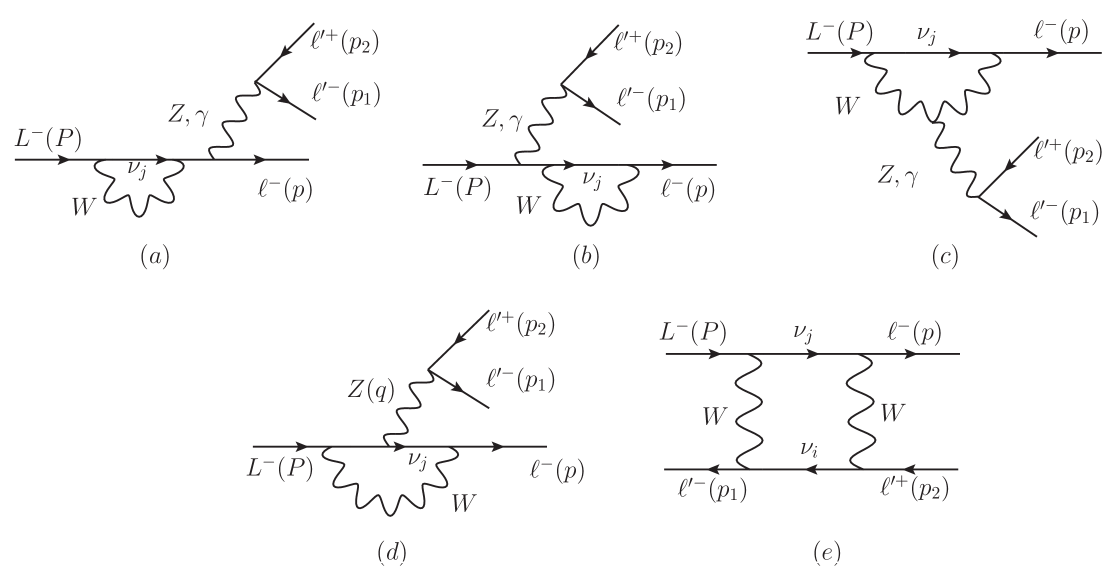
The $L^{-}\to\ell^{-}\ell^{\prime-}\ell^{\prime+}$ decays can be induced through the diagrams depicted in fig. 1. Since the main purpose of this work is to falsify the existence of the logarithmic divergent term claimed in ref. Pham:1998fq , we first concentrate on the amplitude of the diagram (d). We have, however, verified the corresponding expressions for the loop integrals in ref. Petcov:1976ff for the particular process $\mu^{-}\to e^{-}e^{-}e^{+}$, when masses and momenta of external leptons are neglected in the computations. Particularly, in Ref. Petcov:1976ff it is shown that the corresponding branching ratio is completely dominated by those diagrams with two neutrino propagators, i. e. (d) and (e) in fig. 1, which contribute comparably.

In our analysis, we keep employing the convention used by ref. Pham:1998fq , in order to denote the masses and momenta (see fig. 1) of the external leptons, that is $M$ and $P$ ($m$ and $p$) stand for the mass and momentum of the $L^{-}$ ($\ell^{-}$) lepton, respectively. In this way, the amplitude of the diagram (d) can be written as

$\displaystyle\mathcal{M}_{d}$

$\displaystyle\sim$

$\displaystyle\frac{i}{m_{Z}^{2}}l_{L\ell}^{\lambda}\times\ell_{\ell^{\prime}\ell^{\prime}\lambda},$

(1)

where $\ell_{\ell^{\prime}\ell^{\prime}}^{\lambda}=-ig/(2c_{W})\bar{u}(p_{1})\gamma^{\lambda}(g_{v}^{\ell^{\prime}}-g_{a}^{\ell^{\prime}}\gamma_{5})v(p_{2})$ ²²2$g$ is the $SU(2)_{L}$ coupling and $c_{W}(s_{W})$ is short for the cosine(sine) of the weak mixing angle $\theta_{W}$. In the SM, $g_{v}^{\ell^{\prime}}=-1/2+2s_{W}^{2}$ and $g_{a}^{\ell^{\prime}}=-1/2$. is independent of the loop integration, whereas the relevant part for the latter is given by the effective $ZL\ell$ transition as follows:

$$l_{L\ell}^{\lambda}=\left(\frac{-ig}{4c_{W}}\right)\left(\frac{-ig}{2\sqrt{2}}\right)^{2}\sum_{j=1}^{3}U^{*}_{\ell j}U_{Lj}\bar{u}(p)\Gamma^{\lambda}_{j}u(P),$$

(2)

where $U_{im}$ are entries of the PMNS mixing matrix. In the Feynman-’t Hooft gauge we have

$$\Gamma^{\lambda}_{j}=\int\frac{d^{4}k}{(2\pi)^{4}}\frac{\gamma_{\rho}(1-\gamma_{5})i\left[(\not{p}+\not{k})+m_{j}\right]\gamma^{\lambda}(1-\gamma_{5})i\left[(\not{P}+\not{k})+m_{j}\right]\gamma_{\sigma}(1-\gamma_{5})(-ig^{\rho\sigma})}{\left[(p+k)^{2}-m_{j}^{2}\right]\left[(P+k)^{2}-m_{j}^{2}\right]\left[k^{2}-m_{W}^{2}\right]}.$$

(3)

After making the loop integration using dimensional regularization in order to deal with the (logarithmic) UV divergences, the Lorentz structure for the $\Gamma^{\lambda}_{j}$ factor can be written as follows,

	$\displaystyle\Gamma^{\lambda}_{j}$	$\displaystyle=$	$\displaystyle F_{a}\gamma^{\lambda}(1-\gamma_{5})+F_{b}\gamma^{\lambda}(1+\gamma_{5})+F_{c}(P+p)^{\lambda}(1+\gamma_{5})$		(4)
		$\displaystyle+$	$\displaystyle F_{d}(P+p)^{\lambda}(1-\gamma_{5})+F_{e}q^{\lambda}(1+\gamma_{5})+F_{f}q^{\lambda}(1-\gamma_{5}),$

where in general $F_{k}=F_{k}(q^{2},m_{j}^{2})$ $(k=a,\,b...,\,f)$ are functions given in terms of the momentum transfer $q^{2}$, and the neutrino mass squared (of course $F_{k}$ functions will also depend on the mass of the $W$ gauge boson and external masses, but these have well-defined values).

At this point, it is worth to note that in the approximation where the momenta of the external particles are neglected in equation (3), such as it is done in ref. Petcov:1976ff for the $\mu\to 3e$ decay, the computation is simplified considerably, as the only possible contribution is given by the $F^{0}_{a}$ function, where we are using a superscript $0$ in order to distinguish this approximation. In this simple case, the $F^{0}_{a}$ function will not depend on $q^{2}$ and is given in terms of the Feynman parameters as follows

$$F^{0}_{a}(m_{j}^{2})=\frac{1}{2\pi^{2}}\int_{0}^{1}\int_{0}^{1-x}\left[2+\log\left(D^{0}_{j}/\mu^{2}\right)\right]dxdy,$$

(5)

where $D^{0}_{j}(m_{j}^{2})=(1-x)m_{j}^{2}+xm_{W}^{2}$. Whereas in terms of PaVe functions it is given by

	$\displaystyle F^{0}_{a}(m_{j}^{2})$	$\displaystyle=$	$\displaystyle-\frac{1}{8\pi^{2}\left(m_{j}^{2}-m_{W}^{2}\right){}^{2}}\left[2m_{j}^{2}\left(m_{j}^{2}-2m_{W}^{2}\right)B_{0}(0,m_{j}^{2},m_{j}^{2})+2m_{W}^{4}B_{0}(0,m_{W}^{2},m_{W}^{2})\right.$		(6)
		$\displaystyle+$	$\displaystyle\left.4m_{j}^{2}m_{W}^{2}-3m_{j}^{4}-m_{W}^{4}\right].$

Now, one analytical expression for the $F_{a}^{0}$ function can be obtained in a straightforward way either integrating over the Feynman parameters in eq. (5) or using the definition of the $B_{0}(0,m^{2},m^{2})$ scalar function in eq. (6). In such a way that after making an expansion around $m_{j}^{2}=0$ we obtained

$$F^{0}_{a}=\frac{1}{2\pi^{2}}\left[\frac{m_{j}^{2}}{m_{W}^{2}}\log\left(\frac{m_{W}^{2}}{m_{j}^{2}}\right)-\frac{m_{j}^{2}}{2m_{W}^{2}}+\frac{1}{2}\log\left(\frac{m_{W}^{2}}{\mu^{2}}\right)+\frac{1}{4}+\vartheta\left(\frac{m_{j}^{2}}{m_{W}^{2}}\right)^{2}\right].$$

(7)

From eq. (7) it turns clear that, in this approximation, the amplitude will be proportional to the neutrino mass squared, where the dominant contribution, due to the big gap between the neutrino and $W$ boson mass scales, comes from the first term as it involves a relative factor $\log\left(\frac{m_{W}^{2}}{m_{j}^{2}}\right)$ compared to the second one ³³3A similar relative suppression operates for the diagrams in fig. 1 (a), (b) and (c) with respect to the diagrams in fig. 1 (d) and (e)., whereas the independent terms on neutrino mass will vanish by the GIM-like mechanism.

Therefore, the structure of the matrix element for the contribution of the diagram (d) in fig. 1 in the approximation where masses and momenta of the external particles are neglected is given by

	$\displaystyle\mathcal{M}_{d}$	$\displaystyle=$	$\displaystyle-i\frac{G_{F}^{2}m_{W}^{2}\beta_{F^{0}_{a}}}{4}\,\bar{u}(p)\gamma_{\lambda}(1-\gamma_{5})u(P)\times\bar{u}(p_{1})\gamma^{\lambda}(1-\gamma_{5})v(p_{2})$		(8)
		$\displaystyle+$	$\displaystyle iG_{F}^{2}m_{W}^{2}s_{W}^{2}\beta_{F^{0}_{a}}\,\bar{u}(p)\gamma_{\lambda}(1-\gamma_{5})u(P)\times\bar{u}(p_{1})\gamma^{\lambda}v(p_{2})\,,$

where we have defined

$$\beta_{F^{0}_{a}}=\sum_{j}U_{Lj}U^{*}_{\ell j}F^{0}_{a}(m_{j}^{2}).$$

(9)

We verified that eq. (8) reproduces the result reported in ref. Petcov:1976ff considering only the first term in eq. (7) and the simple case of two families.

Returning to the general case (non-zero masses and momentum of the external particles), we also have obtained the $F_{k}$ functions using both Feynman parametrization (we will denote the corresponding expressions by $F_{F_{k}}$) and the Passarino-Veltman (PaVe) technique (denoted by $F_{PV_{k}}$) tHooft:1978jhc ; Passarino:1978jh , employing FeynCalc Mertig:1990an . In particular, we agree with the expressions previously reported in ref. Pham:1998fq in terms of the Feynman parameters ⁴⁴4We have found some irrelevant differences in the numerators of the $f_{d}$ and $f_{f}$ functions, as can be seen comparing eqs. (11), (12) and (13) with the corresponding expressions in ref. Pham:1998fq ., namely the $F_{F_{k}}$ functions can be written as

$$F_{F_{k}}(q^{2},m_{j}^{2})=\frac{1}{2\pi^{2}}\int_{0}^{1}dx\int_{0}^{1-x}f_{k}(q^{2},m_{j}^{2})dy,$$

(10)

where

	$\displaystyle f_{a}$	$\displaystyle=$	$\displaystyle 2+\log\left(D_{j}(q^{2})/\mu^{2}\right)+\frac{(q^{2}-m^{2})x(y-1)+M^{2}x(x+y)+q^{2}y(y-1)}{D_{j}},$		(11)
	$\displaystyle f_{b}$	$\displaystyle=$	$\displaystyle\frac{mMx}{D_{j}},\quad f_{c}=-\frac{Mx(x+y)}{D_{j}},\quad f_{d}=-\frac{mx(1-y)}{D_{j}},$		(12)
	$\displaystyle f_{e}$	$\displaystyle=$	$\displaystyle\frac{Mx(2-3y-x)-2My(y-1)}{D_{j}},\quad f_{f}=\frac{xm(y-1)+2my(y-1)}{D_{j}},$		(13)

and $D_{j}$ is defined as

$$D_{j}(q^{2},m_{j}^{2})=-(x-1)m_{j}^{2}-m^{2}xy+xm_{W}^{2}+M^{2}x(x+y-1)-q^{2}y(1-x-y).$$

(14)

We have omitted in $f_{a}$ the term associated with the UV divergence since it is independent of $m_{j}$ and vanishes owing to the GIM-like mechanism.

On the other hand, the $F_{k}$ functions in terms of the PaVe scalar functions are given as follows

$$F_{PV_{k}}(q^{2},m_{j}^{2})=\frac{1}{2\pi^{2}}\frac{N_{F_{k}}}{D_{F_{k}}},$$

(15)

with

	$\displaystyle D_{F_{a}}=2D_{F_{b}}$	$\displaystyle=$	$\displaystyle-2\lambda(m^{2},M^{2},q^{2}),$		(16)
	$\displaystyle D_{F_{c}}=D_{F_{e}}$	$\displaystyle=$	$\displaystyle\frac{M}{2}D_{F_{a}}^{2}\quad D_{F_{d}}\,=\,D_{F_{f}}\,=\,\frac{m}{2}D_{F_{a}}^{2}\,,$		(17)

	$\displaystyle N_{F_{k}}$	$\displaystyle=$	$\displaystyle\xi_{k_{1}}B_{0}(m^{2},m_{j}^{2},m_{W}^{2})+\xi_{k_{2}}B_{0}(M^{2},m_{j}^{2},m_{W}^{2})+\xi_{k_{3}}B_{0}(q^{2},m_{j}^{2},m_{j}^{2})+\xi_{k_{4}}B_{0}(0,m_{j}^{2},m_{W}^{2})$		(18)
			$\displaystyle+\xi_{k_{5}}C_{0}(m^{2},M^{2},q^{2},m_{j}^{2},m_{W}^{2},m_{j}^{2})+\xi_{k_{0}},$

where $\lambda$ is the Kallen function $\lambda(x,y,z)=x^{2}+y^{2}+z^{2}-2(xy+xz+yz)$, and the $\xi_{k}$ factors can be found in the appendix A.⁵⁵5The cancellation of the UV divergences for the $F_{m}$ functions in terms of the PaVe functions occurs again by the GIM mechanism. This can be verified easily owing to the fact that the sums over the coefficients of the different scalar $B_{0}$ functions, which contain an isolated divergent term, are independent of $m_{j}$. That is $\sum_{i=1}^{4}\frac{\xi_{a_{i}}}{D_{PV_{a}}}=-\frac{1}{2}$, and $\sum_{i=1}^{4}\frac{\xi_{l_{i}}}{D_{PV_{l}}}=0$ for ($l=b,c,d,e,f$).

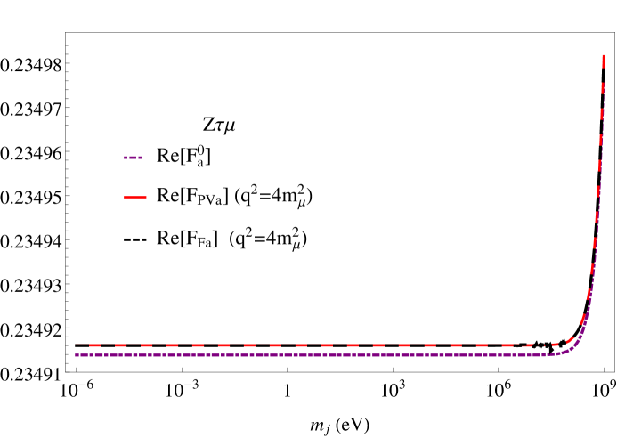
Unlike the approximation made in ref. Petcov:1976ff , the presence of masses and momenta of the external particles in the computation hinders the way for the derivation of analytical expressions for the integrals in eqs. (10) or (15)  ⁶⁶6The analytical expressions of the first integrals over the $y$ parameter in eqs. (11), (12) and (13) can be derived from the formulas reported in appendix B.. Nevertheless, we have done a numerical cross-check between both expressions, where we have employed the Looptools package vanOldenborgh:1989wn ; Hahn:1998yk for the evaluation of the PaVe functions and a numerical Mathematica Mathematica routine for the evaluation of the parametric integrals (see fig. 2). We have found an excellent agreement between these two expressions for values of $q^{2}<4m_{j}^{2}$, which are, however, out side of the physical domain for the considered decays, since $q^{2}_{\rm{min}}=4m_{\ell^{\prime}}^{2}\gg m_{j}^{2}$. In this way, owing to the simpler integrals, we verified that a better precision is found in terms of PaVe functions than using Feynman parameters, this feature is illustrated, as an example, for the particular case of the $Z\tau\mu$ transition in fig. 2 for the (dominant, as we will show) $F_{a}$ factor.

At this point, we want to stress that we disagree with the approximation done in ref. Pham:1998fq in order to estimate the relevant dependence on the neutrino mass of the $F_{k}$ functions. We highlight that we are studying a process where the momentum transfer $q^{2}$ must be non-vanishing and in principle is much larger than the neutrino squared mass, $m_{j}^{2}$, which comes from the loop computation. Therefore, using an expansion around $q^{2}=0$ in order to simplify the integration over the Feynman parameters keeping the terms proportional to $m_{j}^{2}$ in the denominators of equations (11), (12) and (13), as it is done in ref. Pham:1998fq , modifies substantially the behavior of the original functions in the interesting physical region for the neutrino masses and, as a consequence, it gives rise to an incorrect infrared logarithmically divergent behavior of the $F_{k}$ functions when $m_{j}$ goes to zero, without any possible cure. In particular, the dependence on the momentum transfer, $q^{2}$, plays a crucial role in the behavior of the $F_{k}$ functions. In this respect, we point out the presence of a small imaginary part in the $F_{a}$ function, which emerges for the physical values $4m_{j}^{2}<q^{2}$.

As we mentioned before, the $q^{2}$ minimum in the $L^{-}\to\ell^{-}\ell^{\prime-}\ell^{\prime+}$ decay is given by $4m_{\ell^{\prime}}^{2}$, which is much larger than neutrinos masses. This, together with the difficulties in obtaining analytical expressions directly for the $F_{k}$ functions suggests employing some numerical approximation to deal with the problem. Because of this, we approximate the $F_{k}$ functions in the physical region for the neutrinos masses by fitting the curves for the real and imaginary parts of the $F_{k}$ functions evaluated in terms of the PaVe function ⁷⁷7Our fits for the $F_{k}$ functions are taken with the precision of the Looptools package considering a neutrino mass varying from $10^{-15}$ GeV to the benchmark point $m_{\mu}$ ($m_{e}$), for a fixed value of $q^{2}=4m_{\mu}^{2}$ ($q^{2}=4m_{e}^{2}$) for the $Z\tau\mu$ ($Z\tau e$ and $Z\mu e$) vertices.. We have found a reasonably good fit of the form

$\displaystyle F_{k}$

$\displaystyle=$

$\displaystyle\frac{1}{2\pi^{2}u}\left(Q_{k}+\frac{m_{j}^{2}}{m_{W}^{2}}R_{k}\right),$

where $u=1$ for $k=a,b$ and $u=M$ for $k=c,d,e,f$ and the respective values for the $Q_{k}=Q_{R_{k}}+iQ_{R_{I}}$ and $R_{k}=R_{R_{k}}+iR_{R_{I}}$ factors of all considered channels are given in appendix D.

From eq. (LABEL:fit), it turns clear that the $Q_{k}$ factors will not contribute owing to the GIM-like mechanism, whereas the relevant contributions is given by the $R_{k}$ factors. Then, according to our numerical results, we find that the relevant factors of the $F_{b}$, $F_{c}$ and $F_{d}$ functions are suppressed with respect to the $F_{a}$ factor. On the other hand, despite the respective factors of $F_{e}$ and $F_{f}$ functions are larger than those of the $F_{a}$ function, when the momentum transfer becomes smaller and smaller their helicity suppression makes them negligible. Therefore, we will concentrate on the contribution of the $F_{a}$ function. Furthermore, in order to justify our results, we have made an expansion for the PaVe functions involved in eq. (18), following the same strategy that Cheng and Li for the $\mu\to e\gamma$ decay LibroCheng , that is expanding the loop integrals around $m_{j}^{2}=0$ (more details of our expansions are given in appendix E), and with the help of Package-X program Patel:2015tea , we have been able to rewrite the $F_{PV_{a}}$ contribution as follows,

$$F_{PV_{a}}(q^{2},m_{j}^{2})=\frac{1}{2\pi^{2}}\left[Q_{a}+\frac{m_{j}^{2}}{m_{W}^{2}}R_{a}+\vartheta\left(\frac{m_{j}^{4}}{m_{W}^{4}}\right)\right],$$

(20)

where

	$\displaystyle Q_{a}$	$\displaystyle=$	$\displaystyle-\lambda(m^{2},M^{2},q^{2})^{-1}\left[f_{Q_{a_{1}}}C_{0}(m^{2},M^{2},q^{2},0,m_{W}^{2},0)+f_{Q_{a_{2}}}\log\left(\frac{m_{W}^{2}}{m_{W}^{2}-m^{2}}\right)\right.$		(21)
		$\displaystyle+$	$\displaystyle\left.f_{Q_{a_{3}}}\log\left(\frac{m_{W}^{2}}{m_{W}^{2}-M^{2}}\right)+f_{Q_{a_{4}}}\log\left(\frac{m_{W}^{2}}{q^{2}}\right)+f_{Q_{a_{5}}}\right]-\frac{1}{2}\Delta,$

	$\displaystyle R_{a}$	$\displaystyle=$	$\displaystyle-m_{W}^{2}\lambda(m^{2},M^{2},q^{2})^{-1}\left[f_{R_{a_{1}}}C_{0}(m^{2},M^{2},q^{2},0,m_{W}^{2},0)+f_{R_{a_{2}}}\log\left(\frac{m_{W}^{2}}{m_{W}^{2}-m^{2}}\right)\right.$		(22)
		$\displaystyle+$	$\displaystyle\left.f_{R_{a_{3}}}\log\left(\frac{m_{W}^{2}}{m_{W}^{2}-M^{2}}\right)+f_{R_{a_{4}}}\log\left(\frac{m_{W}^{2}}{q^{2}}\right)+f_{R_{a_{5}}}\right],$

where $\Delta=\frac{1}{\textstyle{\epsilon}}-\gamma_{E}+\log(4\pi)$, and the $f_{Q}$ and $f_{R}$ factors can be found in the appendix E. We verified that our numerical fits for the $Z\tau\mu$ and $Z\tau e$ vertex are in a very good agreement with eq. (22), whereas a deviation is found for the $Z\mu e$ vertex, as can be seen in Table 9, we consider the results obtained from eq. (22) for the effective vertices as our reference ones.

In this way, we can approximate the amplitude for diagram (d) according to eq. (8) replacing $F_{a}^{0}$ by

$$F_{a}\approx\frac{1}{2\pi^{2}}\frac{m_{j}^{2}}{m_{W}^{2}}R_{a},$$

(23)

Now, in order to evaluate the respective branching fractions for the $L^{-}\to\ell^{-}\ell^{\prime-}\ell^{\prime+}$ decays we considered the state of the art best fit values of the three neutrino oscillation parameters Patrignani:2016xqp ; Fits . Without lose of generality, we assume the $CP$-conserving scenario ⁸⁸8In general, the leptonic mixing matrix can involve three $CP$-violating phases, one Dirac phase $\delta$, and two additional physical phases in case neutrinos are Majorana particles. Lepton number conserving observables (as those considered here) are not sensitive to the latter, so that for $L^{-}\to\ell^{-}\ell^{\prime-}\ell^{\prime+}$ decays they can only depend on the phase $\delta$. Once the unitarity condition has been used to write the lightest neutrino mass eigenstate contribution in terms of the other two, it can be seen that the term with the largest logarithm (Log$(m_{3}^{2}/m_{1}^{2})$ in the normal hierarchy) has a PMNS pre-factor (we are using the PDG parametrization) which does not depend on $\delta$, which justifies our approach., and we use the following values reported for the mixing angles $\sin^{2}\theta_{12}=0.307(13)$, $\sin^{2}\theta_{23}=0.51(4)$, and $\sin^{2}\theta_{13}=0.0210(11)$, whereas the neutrino mass squared differences are taken as $\Delta m^{2}_{32}=2.45(5)\times 10^{-3}$eV² and $\Delta m^{2}_{21}=7.53(18)\times 10^{-5}$eV^{2 99}9These numbers correspond to the normal hierarchy ($m_{1}<m_{2}<m_{3}$); different (though very similar) values are reported for the inverted hierarchy ($m_{3}<m_{1}<m_{2}$). Changing hierarchy is immaterial for our numerical evaluations. We have verified that results are not sensitive to the lightest neutrino mass value, but only to the mass squared differences.. The kinematics for the $L^{-}\to\ell^{-}\ell^{\prime-}\ell^{\prime+}$ decays can be found in Appendix C.

Neglecting for the moment the box contributions, we get the branching fractions reported in table 1.

Now, in order to make a complete comparison with the approximation done in ref. Petcov:1976ff we have also obtained the amplitude for the box diagram (e) in fig. 1. Note that unlike the penguin diagram (d), which involves two neutrino propagators of the same flavor, the box diagram (e) can involve two neutrino propagators with different flavors. Thus, in full generality, the amplitude can be written as follows

$$\mathcal{M}_{e}=\left(\frac{-ig}{2\sqrt{2}}\right)^{4}\sum_{i,j}U_{Lj}U^{*}_{lj}U_{\ell^{\prime}i}U^{*}_{\ell^{\prime}i}T_{\sigma\sigma^{\prime}}I^{\sigma\sigma^{\prime}},$$

(24)

where we defined

$\displaystyle T_{\sigma\sigma^{\prime}}$

$\displaystyle=$

$\displaystyle 4\,\bar{u}(p)\gamma_{\mu}\gamma_{\sigma}\gamma_{\nu}(1-\gamma_{5})u(P)\times\bar{u}(p_{1})\gamma^{\nu}\gamma_{\sigma^{\prime}}\gamma^{\mu}(1-\gamma_{5})v(p_{2})$

(25)

and the relevant loop integral is given by (see fig. 1 (e))

$$I^{\sigma\sigma^{\prime}}=\int\frac{d^{4}k}{(2\pi)^{4}}\frac{(P+k)^{\sigma}(k+p_{1})^{\sigma^{\prime}}}{(k^{2}-m_{W}^{2})[(p_{1}+p_{2}+k)^{2}-m_{W}^{2}][(P+k)^{2}-m_{j}^{2}][(k+p_{1})^{2}-m_{i}^{2}]}.$$

(26)

Since we have written the equation (26) in terms of $P$, $p_{1}$ and $p_{2}$ momenta the integral must take the form

	$\displaystyle I^{\sigma\sigma^{\prime}}$	$\displaystyle=$	$\displaystyle i\left(g^{\sigma\sigma^{\prime}}H_{a}+P^{\sigma}P^{\sigma^{\prime}}H_{b}+P^{\sigma}p_{1}^{\sigma^{\prime}}H_{c}+P^{\sigma}p_{2}^{\sigma^{\prime}}H_{d}+p_{1}^{\sigma}P^{\sigma^{\prime}}H_{e}\right.$		(27)
		$\displaystyle+$	$\displaystyle\left.p_{1}^{\sigma}p_{1}^{\sigma^{\prime}}H_{f}+p_{1}^{\sigma}p_{2}^{\sigma^{\prime}}H_{g}+p_{2}^{\sigma}P^{\sigma^{\prime}}H_{h}+p_{2}^{\sigma}p_{1}^{\sigma^{\prime}}H_{i}+p_{2}^{\sigma}p_{2}^{\sigma^{\prime}}H_{j}\right).$

The $H_{k}$ factors depend upon the kinematical variables $s_{12}=(p_{1}+p_{2})^{2}=q^{2}$ and $s_{13}=(p_{1}+p)^{2}$, in addition of $m_{i}$ and $m_{j}$.

Anew, in the approximation where momenta of the external particles are neglected in eq. (26), the only contribution is given by the $H^{0}_{a}$ function, which will not depend either on $s_{12}$ or $s_{13}$. In such case, we obtained the following simplified expression

$$H_{a}^{0}(m_{j}^{2},m_{i}^{2})=\frac{1}{16\pi^{2}}\int_{0}^{1}dx\int_{0}^{1-x}dy\int_{0}^{1-x-y}\frac{-1}{2M_{F_{0}}^{2}}dz,$$

(28)

where

$\displaystyle M_{F_{0}}^{2}$

$\displaystyle=$

$\displaystyle m_{W}^{2}(x+y)-m_{j}^{2}(x+y-1)+(m_{i}^{2}-m_{j}^{2})z.$

(29)

Whereas, in terms of PaVe functions, $H^{0}_{a}$ reads

	$\displaystyle H^{0}_{a}(m_{j}^{2},m_{i}^{2})$	$\displaystyle=$	$\displaystyle\frac{1}{16\pi^{2}}\left(\frac{m_{j}^{4}}{4\left(m_{j}^{2}-m_{i}^{2}\right)\left(m_{j}^{2}-m_{W}^{2}\right){}^{2}}B_{0}(0,m_{j}^{2},m_{j}^{2})+\frac{m_{i}^{4}}{4\left(m_{i}^{2}-m_{j}^{2}\right)\left(m_{i}^{2}-m_{W}^{2}\right){}^{2}}B_{0}(0,m_{i}^{2},m_{i}^{2})\right.$		(30)
		$\displaystyle+$	$\displaystyle\left.\frac{2m_{i}^{2}m_{j}^{2}m_{W}^{2}-m_{W}^{4}\left(m_{i}^{2}+m_{j}^{2}\right)}{4\left(m_{i}^{2}-m_{W}^{2}\right){}^{2}\left(m_{j}^{2}-m_{W}^{2}\right)^{2}}B_{0}(0,m_{W}^{2},m_{W}^{2})+\frac{m_{W}^{2}}{4\left(m_{i}^{2}-m_{W}^{2}\right)\left(m_{W}^{2}-m_{j}^{2}\right)}\right)\,.$

In the same way that $F_{a}^{0}$ form factor, an analytical expression for $H_{a}^{0}$ can be obtained easily from either eq. (28) or eq. (30). This time, making a double Taylor expansion, first around $m_{i}^{2}=0$ and then around $m_{j}^{2}=0$, we obtained that

	$\displaystyle H^{0}_{a}(m_{j}^{2},m_{i}^{2})$	$\displaystyle=$	$\displaystyle\frac{1}{64\pi^{2}m_{W}^{4}}\left[\left(m_{i}^{2}+m_{j}^{2}\right)\left(\log\left(\frac{m_{W}^{2}}{m_{j}^{2}}\right)-1\right)\right.$		(31)
		$\displaystyle+$	$\displaystyle\left.\frac{m_{i}^{2}m_{j}^{2}}{m_{W}^{2}}\left(2\log\left(\frac{m_{W}^{2}}{m_{j}^{2}}\right)-1\right)-m_{W}^{2}+\vartheta\left(\frac{m_{i}^{4}}{m_{W}^{2}}\right)+\vartheta\left(\frac{m_{j}^{4}}{m_{W}^{2}}\right)\right].$

Using that $T_{\sigma\sigma^{\prime}}g^{\sigma\sigma^{\prime}}=16\bar{u}(p)\gamma_{\lambda}(1-\gamma_{5})u(P)\times\bar{u}(p_{1})\gamma^{\lambda}(1-\gamma_{5})v(p_{2})$, the amplitude -in this approximation- is given by

$\displaystyle\mathcal{M}_{e}$

$\displaystyle=$

$\displaystyle i8G_{F}^{2}m_{W}^{4}\beta_{H^{0}_{a}}\,\bar{u}(p)\gamma_{\lambda}(1-\gamma_{5})u(P)\times\bar{u}(p_{1})\gamma^{\lambda}(1-\gamma_{5})v(p_{2}),$

(32)

with

$$\beta_{H^{0}_{a}}=\sum_{j,i}U_{Lj}U^{*}_{\ell j}U_{\ell^{\prime}i}U^{*}_{\ell^{\prime}i}H^{0}_{a}(m_{i}^{2},m_{j}^{2}).$$

(33)

Again, we verified that taking into account the first term in eq. (31) and considering only two families, eq. (32) reproduces the expression reported in ref. Petcov:1976ff for the amplitude of the box diagram 1 (e) in the $\mu\to 3e$ decay.

In the general case, we also obtained the $H_{k}$ ($k=a,b,...,j$) functions in terms of both Feynman parameters integrals, $H_{F_{k}}$, and PaVe functions, $H_{PV_{k}}$. This time, the $H_{k}$ functions will depend on the squared masses of two different neutrinos, $m_{j}^{2}$ and $m_{i}^{2}$, and on two independent phase space variables $s_{12}$ and $s_{13}$. Using Feynman parametrization these functions read

$$H_{F_{k}}(s_{12},s_{13},m_{i}^{2},m_{j}^{2})=\frac{1}{16\pi^{2}}\int_{0}^{1}dx\int_{0}^{1-x}dy\int_{0}^{1-x-y}h_{k}(s_{12},s_{13},m_{i}^{2},m_{j}^{2})dz\,,$$

(34)

where

$$h_{a}=-\frac{1}{2M_{F}^{2}},\quad h_{b}=\frac{z(z-1)}{M_{F}^{4}},\quad h_{c}=-\frac{(z-1)(x+z)}{M_{F}^{4}},\quad h_{d}=\frac{y(z-1)}{M_{F}^{4}}\quad h_{e}=-\frac{z(x+z-1)}{M_{F}^{4}}\,,$$

(35)

$$h_{f}=\frac{(x+z-1)(x+z)}{M_{F}^{4}},\quad h_{g}=-\frac{y(x+z-1)}{M_{F}^{4}},\quad h_{h}=\frac{yz}{M_{F}^{4}}\quad h_{i}=-\frac{y(x+z)}{M_{F}^{4}},\quad h_{j}=\frac{y^{2}}{M_{F}^{4}}.$$

(36)

In the previous expressions, the denominator function is given by

	$\displaystyle M_{F}^{2}$	$\displaystyle=$	$\displaystyle-m_{j}^{2}(x+y-1)+m_{\ell^{\prime}}^{2}(x+y-1)(x+y)+m_{W}^{2}(x+y)-s_{12}xy+z^{2}\left(2m_{\ell^{\prime}}^{2}+m^{2}+M^{2}-s_{12}-s_{13}\right)$		(37)
		$\displaystyle+$	$\displaystyle z\left[m_{i}^{2}-m_{j}^{2}+(x+y)\left(3m_{\ell^{\prime}}^{2}-s_{12}-s_{13}\right)-2m_{\ell^{\prime}}^{2}+m^{2}(x-1)+M^{2}(y-1)+s_{12}+s_{13}\right].$

Expressions are rather lengthy in terms of the PaVe functions, so that here we only present the expression for the dominant $H_{a}$ function, which can be written as

$$H_{PV_{a}}(s_{12},s_{13},m_{j}^{2},m_{i}^{2})=\frac{1}{16\pi^{2}}\frac{N_{H_{a}}}{D_{H_{a}}},$$

(38)

with

	$\displaystyle D_{H_{a}}$	$\displaystyle=$	$\displaystyle 4\big{(}m^{4}m_{\ell^{\prime}}^{2}-m^{2}\big{[}M^{2}\big{(}2m_{\ell^{\prime}}^{2}-s_{12}\big{)}+s_{12}\big{(}m_{\ell^{\prime}}^{2}+s_{13}\big{)}\big{]}+M^{4}m_{\ell^{\prime}}^{2}-M^{2}s_{12}\big{(}m_{\ell^{\prime}}^{2}+s_{13}\big{)}$		(39)
		$\displaystyle+$	$\displaystyle s_{12}\big{(}-2s_{13}m_{\ell^{\prime}}^{2}+m_{\ell^{\prime}}^{4}+s_{13}\big{(}s_{12}+s_{13}\big{)}\big{)}\big{)},$

and

	$\displaystyle N_{H_{a}}$	$\displaystyle=$	$\displaystyle\chi_{k_{1}}C_{0}(m^{2},M^{2},s_{12},m_{W}^{2},m_{i}^{2},m_{W}^{2})+\chi_{k_{2}}C_{0}(m_{\ell^{\prime}}^{2},m_{\ell^{\prime}}^{2},s_{12},m_{W}^{2},m_{j}^{2},m_{W}^{2})$		(40)
		$\displaystyle+$	$\displaystyle\chi_{k_{3}}C_{0}(M^{2},m_{\ell^{\prime}}^{2},m^{2}+M^{2}+2m_{\ell^{\prime}}^{2}-s_{12}-s_{13},m_{i}^{2},m_{W}^{2},m_{j}^{2})$
		$\displaystyle+$	$\displaystyle\chi_{k_{4}}C_{0}(m^{2},m_{\ell^{\prime}}^{2},m^{2}+M^{2}+2m_{\ell^{\prime}}^{2}-s_{12}-s_{13},m_{i}^{2},m_{W}^{2},m_{j}^{2})$
		$\displaystyle+$	$\displaystyle\chi_{k_{5}}D_{0}(m^{2},M^{2},m_{\ell^{\prime}}^{2},m_{\ell^{\prime}}^{2},s_{12},m^{2}+M^{2}+2m_{\ell^{\prime}}^{2}-s_{12}-s_{13},m_{W}^{2},m_{i}^{2},m_{W}^{2},m_{j}^{2}).$

where $\chi_{k}$ factors are reported in Appendix A.

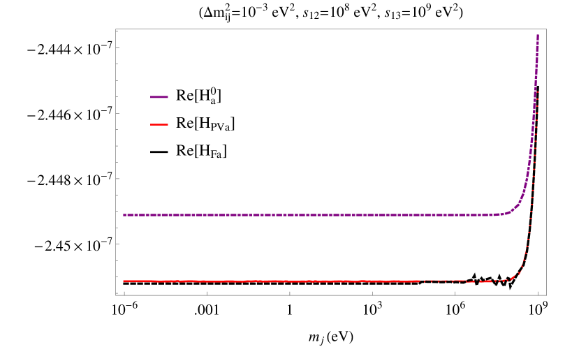
As far as the general case is concerned, we can see that although there are additional contributions associated with the $H_{k}$ functions, with $k=b$, $c$, $d$, $\ldots$ $j$; they are expected to be suppressed, as they correspond to higher-dimensional operators, with respect to the $H_{a}$ function associated with a $(V-A)\times(V-A)$ operator. Therefore, we will concentrate on the $H_{a}$ function in order to estimate the box diagram contribution. We also have done a numerical cross-check between the expressions for the $H_{a}$ function given in terms of the Feynman parameters eq. (34) and the PaVe functions eq. (38), as can be seen in fig. 3. In this case, it turns very complicated and far away of the purpose of this work to obtain an analytical expression for the $H_{a}$ function in eq. (40) making an expansion for the respective scalar PaVe functions, owing to the number of propagators involved and the dependence on two different neutrino masses. However, we can expect a good approximation through our numerical results, such as occurs with the penguin contribution.

References

- (1) S. L. Glashow, Nucl. Phys. 22 (1961) 579; S. Weinberg, Phys. Rev. Lett. 19 (1967) 1264; A. Salam, Conf. Proc. C 680519 (1968) 367.
- (2) Y. Fukuda et al. [Super-Kamiokande Collaboration], Phys. Rev. Lett. 81, 1562 (1998); Q. R. Ahmad et al. [SNO Collaboration], Phys. Rev. Lett. 87, 071301 (2001); 89, 011301 (2002).
- (3) N. Cabibbo, Phys. Rev. Lett. 10 (1963) 531; M. Kobayashi and T. Maskawa, Prog. Theor. Phys. 49 (1973) 652.
- (4) B. Pontecorvo, Sov. Phys. JETP 10 (1960) 1236 [Zh. Eksp. Teor. Fiz. 37 (1959) 1751]; Z. Maki, M. Nakagawa and S. Sakata, Prog. Theor. Phys. 28, 870 (1962).
- (5) S. L. Glashow, J. Iliopoulos and L. Maiani, Phys. Rev. D 2, 1285 (1970).
- (6) T. P. Cheng and L. F. Li, “Gauge Theory Of Elementary Particle Physics,” Oxford, Uk: Clarendon (1984) 536 P. (Oxford Science Publications)
- (7) L. Calibbi and G. Signorelli, Riv. Nuovo Cim. 41, 1 (2018)
- (8) S. T. Petcov, Sov. J. Nucl. Phys. 25, 340 (1977) [Yad. Fiz. 25, 641 (1977)] Erratum: [Sov. J. Nucl. Phys. 25, 698 (1977)] Erratum: [Yad. Fiz. 25, 1336 (1977)].
- (9) B. W. Lee and R. E. Shrock, Phys. Rev. D 16, 1444 (1977).
- (10) X. Y. Pham, Eur. Phys. J. C 8, 513 (1999).
- (11) C. Patrignani et al. [Particle Data Group], Chin. Phys. C 40, 100001 (2016).
- (12) Sw. Banerjee et al [HFLAV-Tau group], available at http://www.slac.stanford.edu/xorg/hflav/tau/spring-2017/tau-report-web.pdf
- (13) I. Esteban, M. C. González-Garcia, M. Maltoni, I. Martínez-Soler and T. Schwetz, JHEP 1701, 087 (2017); F. Capozzi, E. Di Valentino, E. Lisi, A. Marrone, A. Melchiorri and A. Palazzo, Phys. Rev. D 95, 096014 (2017); P. F. de Salas, D. V. Forero, C. A. Ternes, M. Tortola and J. W. F. Valle, Phys. Lett. B 782, 633 (2018)
- (14) E. Kou et al., arXiv:1808.10567 [hep-ex].
- (15) T. Kinoshita, J. Math. Phys. 3 (1962) 650; T. D. Lee and M. Nauenberg, Phys. Rev. 133 (1964) B1549.
- (16) G. Passarino and M. J. G. Veltman, Nucl. Phys. B 160 (1979) 151.
- (17) G. ’t Hooft and M. J. G. Veltman, Nucl. Phys. B 153, 365 (1979).
- (18) R. Mertig, M. Bohm and A. Denner, Comput. Phys. Commun. 64 (1991) 345.
- (19) G. J. van Oldenborgh and J. A. M. Vermaseren, Z. Phys. C 46 (1990) 425.
- (20) T. Hahn and M. Pérez-Victoria, Comput. Phys. Commun. 118 (1999) 153.
- (21) Wolfram Research, Inc., Mathematica, Version 11.3, Champaign, IL (2018).
- (22) J. I. Illana and T. Riemann, Phys. Rev. D 63, 053004 (2001).
- (23) E. Arganda, A. M. Curiel, M. J. Herrero and D. Temes, Phys. Rev. D 71, 035011 (2005).
- (24) H. H. Patel, Comput. Phys. Commun. 197, 276 (2015).