FLEX: an Adaptive Exploration Algorithm for Nonlinear Systems
Abstract
Model-based reinforcement learning is a powerful tool, but collecting data to fit an accurate model of the system can be costly. Exploring an unknown environment in a sample-efficient manner is hence of great importance. However, the complexity of dynamics and the computational limitations of real systems make this task challenging. In this work, we introduce FLEX, an exploration algorithm for nonlinear dynamics based on optimal experimental design. Our policy maximizes the information of the next step and results in an adaptive exploration algorithm, compatible with generic parametric learning models and requiring minimal resources. We test our method on a number of nonlinear environments covering different settings, including time-varying dynamics. Keeping in mind that exploration is intended to serve an exploitation objective, we also test our algorithm on downstream model-based classical control tasks and compare it to other state-of-the-art model-based and model-free approaches. The performance achieved by FLEX is competitive and its computational cost is low.
1 Introduction
Control theory and model-based reinforcement learning have had a range of achievements in various fields including aeronautics, robotics and energy systems (Kirk, 1970; Sutton & Barto, 2018). For the agent to find an effective control policy, the mathematical model of the environment must faithfully capture the dynamics of the system and thus must be fit with data. However, collecting observations can be expensive: consider for example an aircraft system, for which running experiments costs a lot of energy and time (Gupta et al., 1976). In this regard, active exploration (or system identification) aims at exciting the system in order to collect informative data and learn the system globally in a sample-efficient manner (Yang et al., 2021), independent of any control task. Once this task agnostic exploration phase is completed, the learned model can be exploited to solve multiple downstream tasks.
Dynamics may be complex and generally take the form of a nonlinear function of the state. An example would be air friction, which is essential to consider for an accurate control law, and yet difficult to model from physical principles (Faessler et al., 2018; De Simone et al., 2015). While exploration in linear systems is well understood (Goodwin & Payne, 1977), efficiently learning nonlinear dynamics is far more challenging. For realistic applications, this is compounded by the hard limitations of memory and computational resources of embedded systems (Tassa et al., 2012). Furthermore, the dynamics or the agent’s model of it may vary over time, and the exploration policy must adapt as the data stream is collected. Therefore, it is critical that the algorithm works adaptively, with limited memory storage and that it runs fast enough to be implementable in a real system, while being flexible enough to learn complex dynamics with potentially sophisticated models.
Different approaches have been proposed recently for exploring nonlinear environments, and have proceeded by maximizing an information gain (or uncertainty) on the parameters for specific classes of learning models. An exact computation can be derived for models with linear parametrizations (Schultheis et al., 2020), which are however of limited expressivity. Uncertainty can also be computed with Gaussian processes (Buisson-Fenet et al., 2020) or approximated using ensembles of neural networks (Shyam et al., 2019; Sekar et al., 2020) but these approaches suffer from a quadratic memory complexity and an important computational cost respectively, making them unlikely to be implementable in real systems. In all the above approaches, the inputs are planned episodically by solving a non-convex optimization problem where the nonlinear dynamics are simulated over a potentially large time horizon. Planning then relies on nonlinear solvers, which may be too slow to run in real time (Kleff et al., 2021). Furthermore, planning over large time horizons renders the algorithm unable to adapt to new observations as they are collected. As a result, the agent may spend a long time trusting a wrong model and exploring uninformative states. Recent works have focused on deriving a fast and adaptive exploration policy for linear dynamics (Blanke & Lelarge, 2022). However, maintaining such guarantees while exploring substantially more complex systems remains a significant challenge and an open area of research.
Contributions
The present study examines the problem of active exploration of nonlinear environments, with great importance attached to the constraints imposed by real systems. Based on information theory and optimal experimental design, we define an exploration objective that is valid for generic parametric learning models, encompassing linear models and neural networks. We derive an online approximation of this objective and introduce FLEX, a fast and adaptive exploration algorithm. The sample-efficiency and the adaptivity of our method are demonstrated with experiments on various nonlinear systems including a time-varying environment and the performance of FLEX is compared to several baselines. We further evaluate our exploration method on downstream exploitation tasks and compare FLEX to model-based and model-free exploration approaches.
Organization
We first introduce the mathematical formalism of our problem in Section 2. In Section 3, we focus on models with linear parametrizations, for which an information-theoretic objective can be derived. In Section 4, we introduce FLEX (Algorithm 2), our exploration algorithm that adaptively maximizes this objective online. In Section 5, we extend our approach to generic, nonlinear models. We test our method experimentally in Section 6.
2 Exploring a nonlinear environment
In nonlinear dynamical systems, the state and the input are governed by an equation of the form
| (2.1) |
where is a nonlinear function modeling the dynamics. This function is unknown or partially unknown, and our objective is to learn it from data, with as few samples as possible. What is observed in practice is a finite number of discrete, noisy observations of the dynamics (2.1):
| (2.2) |
where is a known time step, is the number of observations, is the state vector, is a normally distributed isotropic noise with known variance , and the control variables are chosen by the agent with the constraint . We assume that is a differentiable function. We write indifferently or where is the state-action pair. Note that our problem could be formulated in the framework of continuous Markov decision processes (Sutton & Barto, 2018), but we find (2.2) more suitable for our approach.
Sequential learning
The dynamics function is learned from past observations with a parametric function , whose parameters are gathered in a vector . We denote a generic parametric model by a map . At each time , the observed trajectory yields an estimate following a learning rule , such as maximum likelihood. At the end of the exploration, the agent returns a final value . Although this learning problem is rich and of an independent interest, we will adopt simple, bounded-memory, online learning rules and focus in this work on the following decision making process.
Sequential decision making
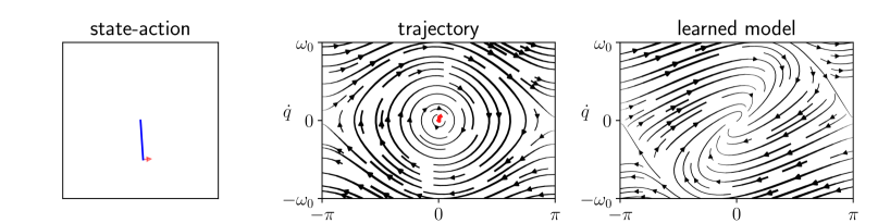
The agent’s decision takes the form of a policy , mapping the past trajectory to the future input, knowing the current parameter . We denote by the set of policies satisfying the constraint of amplitude . The sequential decision making process is summarized in Algorithm 1 and illustrated in Figure 1. The goal of active exploration is to choose inputs that make the trajectory as informative as possible for the estimation of with , as stated below.
The problem
For an arbitrary learning model of the dynamics provided with a learning rule and for a fixed number of observations , the goal is to find an exploration policy for which the learned model is as close to as possible at the end of exploration. Formally, we define the estimation error of parameter as
| (2.3) |
and look for a policy yielding the best estimate of at time :
| (2.4) |
where the expectation is taken over the stochastic dynamics (2.1) and possibly the randomness induced by the policy.
Practical considerations
In addition to the sample efficiency objective (2.4), we attach great importance to the three following practical points that emerge from the observations of Section 1. Adaptivity: as opposed to episodic planning for which remains constant with respect to throughout long time intervals, we want our policy to accommodate to new observations at each time step. Computational efficiency: evaluating the policy should require limited computational resources. Flexibility: our policy should be valid for a broad class of models , as we will see with the following examples.
Example 2.1 (Damped pendulum).
The angle of a pendulum driven by a torque satisfies the following nonlinear differential equation:
| (2.5) |
This second-order system can be described by the bidimensional state variable and the nonlinear map .
Example 2.2 (Nonlinear friction).
Using the same notations, the dynamics of a mass subject to a control force and friction is given (in the case of one-dimensional system for simplicity) by . The friction force is notoriously difficult to model. One possibility would be the nonlinear function (Zhang et al., 2014).
The choice of model is crucial and depends on prior knowledge about the system. In Example 2.1, if the system is known down to its scalar parameters, learning the dynamics reduces to linear regression. In the opposite case where little or nothing is known about the structure, as in Example 2.2, it would be desirable to fit more sophisticated parametric models. For instance, the recent successes of neural networks and their ability to express complex functions and to be trained online make them a promising option for our exploration task (Goodfellow et al., 2016).
Importantly, the exploration policy should depend on the learned model and drive the system to regions with high uncertainty. In contrast, random exploration fails to explore nonlinear systems globally: typically, friction forces pull the system toward a fixed point, while learning the environment requires large amplitude trajectories and hence temporal coherence in the excitation.
3 Information-theoretic view of exploration
Given a model of the dynamics, how do we choose inputs that efficiently navigate in phase space towards informative states ? This choice should be guided by some measure of the information that the trajectory provides about our learning model. In this section, we turn to information theory and study the simplest form of models: linear models provide us not only with a natural learning rule but also with an information-theoretic measure of exploration. We then leverage this criterion to define an optimization objective.
3.1 Linear models
An important class of models is the class of functions with an affine dependence on the parameters. In the remainder of this work, we use the word “linear” for an affine dependence. Note that the term “linear” refers to the parameter dependence of a model, but the dependence in the state-action pair is still assumed to be nonlinear in general.
Definition 3.1 (Linear model).
The most general form for a linear dependence of in its parameters is
| (3.1) |
where the features and are independent of . We denote by the rows of , and we define .
The class of linear models is critically important for several reasons. First, the dynamics can very often be formulated as an affine function of some well-defined scalar parameters, hence allowing for efficient estimation by ordinary least squares (Tedrake, 2022). Besides, a natural mathematical exploration objective from optimal experimental design theory can be derived for linear models (see Section 3.2). Finally, the computations allowed for linear models can be generalized to nonlinear models, as we will see in Section 5.
Example 3.1 (Learning the pendulum).
An important case of linear models is when the parameters are separated in a matrix form according to row-wise dependence, as follows.
Definition 3.2 (Matrix model).
We call a matrix model a parametrization of the form
| (3.3) |
where is a feature map and is a parameter matrix. The structure (3.1) is recovered by defining as the vectorization of of size , and the features as the block matrix .
Example 3.2 (Linear dynamics).
Consider the case of a linear time-invariant system: . A natural parametrization is , with the parameters . This is a matrix model (3.3) where and .
3.2 Optimal experimental design
Let be an observation whose distribution depends on a parameter and a decision variable (or design) denoted . Experimental design theory provides a quantitative answer to the question: how informative are the observations for estimating when the decision is taken? The information is defined as a scalar functions of the Fisher information matrix (Fedorov, 2010) as follows.
Definition 3.3 (Fisher information and information gain).
We denote the log-likelihood of the distribution. The observed Fisher information matrix (Gelman et al., 2004) of observation at some parameter value is
| (3.4) |
The D-optimal information gain is defined as
| (3.5) |
Example 3.4 (Linear regression).
In a linear regression, is the regressor and with the noise , yielding and .
This information gain quantifies the information about provided by the observations with design , and it may be interpreted as the volume of the confidence ellipsoid for the parameter vector . Several other functionals can be used instead of , leading to other optimality criteria. The D-optimality criterion benefits from a property of scale invariance (Pukelsheim, 2006) and is suitable for our online setting because it provides a simple rank-one update formula, as we will see in Section 4. A D-optimal design maximizes the information gain:
| (3.6) |
From a Bayesian perspective, D-optimality minimizes the entropy of the expected posterior on , or equivalently the mutual information between the current prior and the expected posterior (Chaloner & Verdinelli, 1995).
3.3 Optimally informative inputs for exploration
In this section, we apply the optimal experimental design framework to our dynamical setting, where the Gaussian noise assumption and the linear structure of the model allow for exact computations. The observations are the trajectory and the design is the policy generating the inputs .
Definition 3.4 (Gram matrix).
An important quantity is the Gram matrix of the features, defined as
| (3.7) |
Proposition 1.
Assume a linear model (3.1) for the data-generating distribution of the trajectory, with for simplicity. Then, the maximum likelihood estimate of is
| (3.8) |
and the Fisher information matrix is
| (3.9) |
Note that does not depend explicitly on but only on the observations, because the model is linear in the parameters.
It follows from (3.6) and Proposition 1 that, in our setting, D-optimal inputs solve the following optimal control problem:
| (3.10) | ||||
| subject to | ||||
where we neglect the noise in the dynamics for simplicity, and recall that .
Remark 3.1 (Optimal design for matrix models).
For models of the form (3.3), one can readily show that an equivalent objective is obtained by defining instead of .
3.4 Sequential learning
Linear models can be learned online with the recursive least squares formula for the estimator (3.8). Assuming for simplicity , and denoting , online learning takes the form
| (3.11a) | ||||
| (3.11b) | ||||
with the squared error loss and the matrix step size . Equation (3.11b) makes it transparent that recursive least squares is an online gradient descent step. The memory cost of learning is for the storage of and . For , there is one update for each row, hence updates per time step .
4 Adaptive D-optimal exploration with FLEX
We adopt D-optimality (3.10) as an objective for our exploration policy. However, this problem is non-convex and providing a numerical solution is computationally challenging. Furthermore, the dynamics constraint is unknown and can only be approximated with the current knowledge of the dynamics, which is improved at each time step. Although previous approaches have opted for an episodic optimization with large time horizons (Wagenmaker et al., 2021; Schultheis et al., 2020), it is desirable to update the choice of inputs at the same frequency as they are collected. In this section, we introduce FLEX (Algorithm 2), an adaptive D-optimal exploration algorithm with low computational complexity. In this section, we use the notations of linear models as defined in Section 3. We will show how this formalism extends to arbitrary, nonlinear models in Section 5.
4.1 One-step-ahead information gain
Since we seek minimal complexity and adaptivity, we choose to devote the computational effort at time to the choice of the next input only. We want to define an informativeness measure for input and solve a sequence of problems of the form
| (4.1) | ||||
As stated before, we attach great importance to the computational time of solving (4.1).
The function should quantify the information brought by , for which we derived a mathematical expression in our information-theoretic considerations of Section 3. Therefore, we want the problem sequence (4.1) to be an approximation of the problem (3.10).
A greedy approximation can be derived as follows. At time , the past trajectory is known and the choice of immediately determines the next state . We define as the predicted information gain truncated at .
Definition 4.1 (Predicted information gain).
Letting be the one-step-ahead state prediction and , we define
| (4.2) |
with
| (4.3) |
When is of rank one, a simpler formula can be derived.
Lemma 4.1 (Determinant Lemma).
By choosing a row for of the feature matrix and approximating , the expression for the information gain can be simplified as follows:
| (4.4) |
We adopt the rank-one approximation of Lemma 4.1 in the remainder of this work. Note that the index of row can be either drawn randomly or chosen using prior knowledge: the -th row of is informative if the -th component of the model is sensitive with respect to the parameters. One could also design a numerical criterion for this choice.
4.2 Computing D-optimal inputs
For linear systems, recent approaches have shown that a greedy D-optimal policy yields good exploration performance (Blanke & Lelarge, 2022). However for nonlinear systems, the nonlinearity of makes the maximization problem (4.1) challenging. To obtain a simpler optimization problem, we linearize the model with respect to the state. Intuitively, since we are planning between and , the corresponding change in the state is small so it is reasonable to use a linear approximation to the mapping .
Proposition 2.
Remark 4.1 (Linear dynamics).
Our exploration policy is summarized in Algorithm 2. Note that since it optimizes a greedy objective at each time step, it is adaptive by nature and it does not require the knowledge of the time horizon . The following result shows that solving (4.5) can be achieved at low cost, ensuring that our policy is computationally efficient.
Proposition 3.
Problem (4.5) can be solved numerically at the cost of a scalar root-finding and a matrix eigenvalue decomposition.
5 From linear models to nonlinear models
For the cases when no prior information is available about the structure of the dynamics (see Example 2.2), it is desirable to generalize the policy derived in Section 4 to more complex models that are not linear in the parameters. In this section, we extend Algorithm 2 to generic, nonlinear parametric models. We assume that is doubly differentiable with respect to and .
5.1 Linearized model
The developments of Section 4 are based on the linear dependence of the model on the parameters. For nonlinear models, a natural idea is to make a linear expansion of the model: assuming that the parameter vector is close to a convergence value , we can linearize to first order in :
| (5.1) |
In the limiting regime where this linear approximation would hold, would be a linear model with features
| (5.2) |
5.2 Online exploration with nonlinear models
In our dynamical framework, we expect the approximation (5.1) to be increasingly accurate as more observations are collected, hence motivating the generalization of the exploration strategy developed in Section 4 to nonlinear models. The features of the linearized model (5.1) are unknown because the Jacobian (5.2) depends on the unknown parameter in general. However, we can approximate by the current estimate at each time step along the trajectory. By defining
| (5.3) |
we extend the notion of the Gram matrix in Definition 3.4 as well as the optimal control problem (3.10) to nonlinear models. Note that since depends only on , the Gram matrix can still be computed online along the trajectory. Similarly, we extend the approach developed in Section 4 by defining
| (5.4) |
with chosen as in Lemma 4.1. With these quantities defined, Algorithm 2 is extended to arbitrary models.
Remark 5.1 (Consistency with linear models).
5.3 Computational perspective
In Algorithm 2, we need to compute , which amounts to computing the derivatives of in both and :
| (5.5) |
For neural networks, this matrix can be computed by automatic differentiation. The cost of solving (4.5) does not depend on so the computation of becomes the computational bottleneck for large models. The complexity of the latter operation is with automatic differentiation.
5.4 Sequential learning
We train nonlinear models using online gradient descent:
| (5.6) |
which extends (3.11b). For neural networks, online learning with an adaptive learning rate (and scalar is known to be effective (Bottou, 2012; Kingma & Ba, 2015). The gradient step can be averaged over a batch for smoother learning, at the cost of storing a small amount of data points.
6 Experiments
We run several experiments to validate our method. Our code and a demonstration video are available at https://github.com/MB-29/exploration. More details about the experiments can be found in Appendix C.
6.1 Exploration benchmark
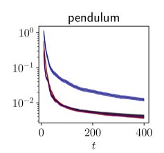
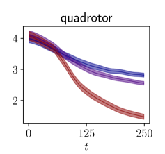
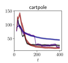
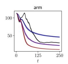
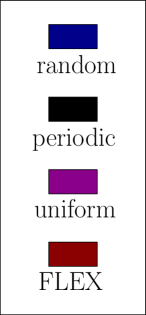
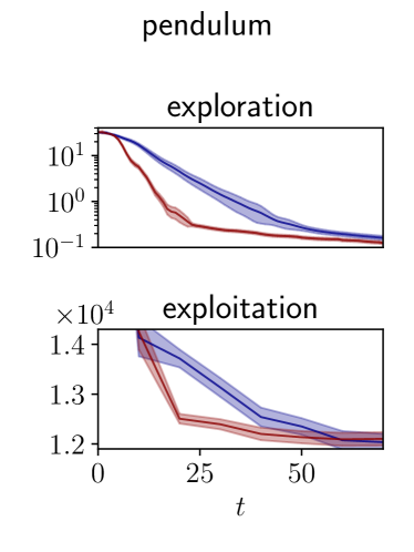
We first test our policy on various nonlinear environments from classical control, covering different values for and . We compare its performance in terms of sample efficiency to that of various baselines. The agents have the same learning model, but different exploration policies. Random exploration draws inputs at random. For pendulum-like environments, a periodic oracle baseline excites the system at an eigenmode, yielding resonant trajectories of large amplitude. A baseline called “uniform” maximizes the distance of the trajectory points in the state space: it optimizes objective (4.2) with .
Experimental setup
The learning models include various degrees of prior knowledge on the dynamics. A linear model is used for the pendulum, and neural networks are used for the other environments. The Jacobians of Proposition 2 are computed using automatic differentiation. At each time step, the model is evaluated with (2.3) computed over a fixed grid.
Results
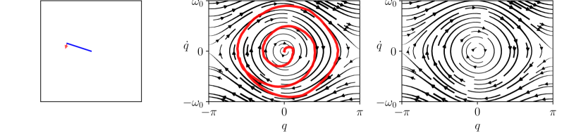
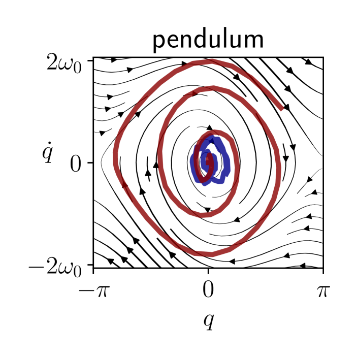
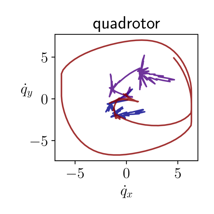
The results are presented in Figure 2. Our algorithm is sample-efficient and it outperforms the baselines in all the environments. We also display the trajectories obtained with our policy in phase space in Figure 3. Not only does FLEX produce informative trajectories of large amplitude, but more specifically it devotes energy so as to explore regions with higher uncertainty, unlike the baselines. Although the policy optimizes the information in a greedy fashion, it interestingly produces inputs with long-term temporal coherence. This is illustrated in our demonstration video. High-dimensional exploration is tackled in Appendix B.
6.2 Tracking of time-varying dynamics
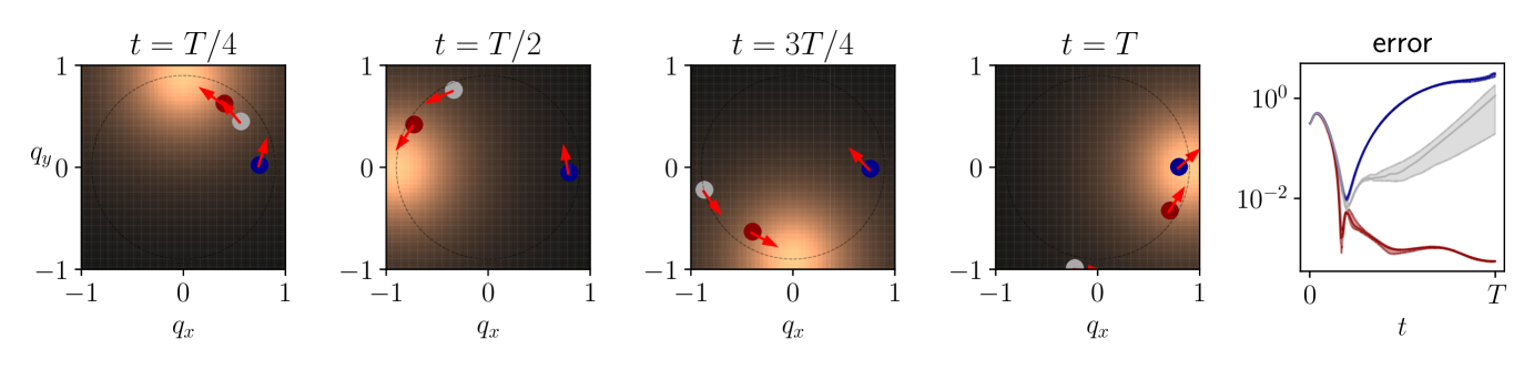

In real systems, dynamics may vary over time and an adaptive exploration is crucial for accommodating to changes in the environment. We test the adaptivity of our method by exploring a time-varying system, and compare to an episodic agent. The system is a central, repulsive force field centered on a star, moving around a circle uniformly at a period . The agent is a spaceship and the control variable is the acceleration. The force field varies significantly only in the vicinity of the star: the spaceship learns information about the dynamics only when it is close, and hence needs to track the star.
Experimental setup
The model learns the center and the radius of the force field, yielding a nonlinear parametrization (see Appendix C.2). With this model, three agents learn the dynamics: a random policy, FLEX, and an episodic agent that plans D-optimal inputs by solving (3.10) over a time horizon of repeatedly. At each time step, the model is evaluated in the parameter space with the distance to the real system parameters at the current time.
Results
The trajectories and the error curves are presented in Figure 4. Although the episodic agent initially follows the star, it eventually loses track of the dynamics because of the delay induced by planning over a time interval. Our adaptive policy, on the other hand, successfully explores the dynamics. Even though the planning of inputs has linear time complexity in in both cases, we observe a slowdown by a factor 100 for the episodic agent. We believe that this experiment on this toy model illustrates the relevance of an adaptive exploration policy in realistic settings.
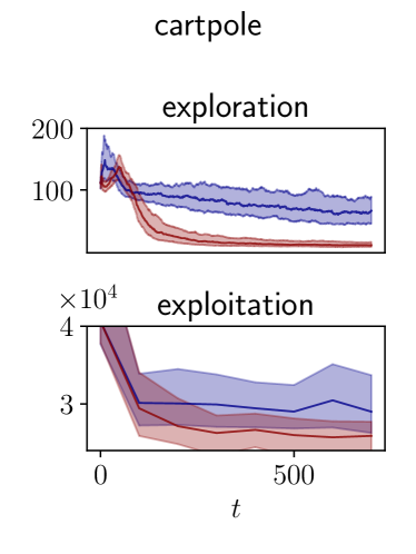
6.3 From exploration to exploitation
The goal of exploration is ultimately to obtain an accurate model for the system for model-based control. In order to validate the relevance of our approach to this framework, we evaluate the model learned during exploration on model-based control tasks. We compare it to the recent active exploration algorithms RHC and MAX (Schultheis et al., 2020; Shyam et al., 2019) and to the model-free reinforcement learning algorithm SAC (Haarnoja et al., 2018).
Experimental setup
We experiment on the pendulum and the cartpole of the DeepMind control suite (Tunyasuvunakool et al., 2020), for which we added noise. Throughout exploration, the learned model is evaluated using both (2.3) and with the exploitation cost achieved by a model-based control algorithm on the swingup task. The experimental details can be found in Appendix C.3 and in (Schultheis et al., 2020) along with the performance of the algorithms used for comparison. The control task is considered solved when the cost is lower than a value that we have chosen arbitrarily based on simulations.
Results
Our results are presented in Table 1 and in Figure 6. Our algorithm is sample-efficient in terms of exploitation, as it allows for a model-based control algorithm to solve the task faster than the other baselines. Its computational cost is low.
| Method | RAND | MAX | SAC | RHC | FLEX |
|---|---|---|---|---|---|
| samples | k | 2000 | k | 500 | 50 |
| compute | 1 | 100 | 2 | 8 | 4 |
| samples | k | k | k | ||
| compute | 1 | 20 | 1.5 | 2 | 1.6 |
7 Related work
The pure exploration task has recently attracted much interest in both the control and the reinforcement learning communities. Several methods have been proposed to learn the dynamics and to model uncertainty, including Gaussian processes (Buisson-Fenet et al., 2020), Random Fourier Features (Schultheis et al., 2020), and neural networks ensembles (Shyam et al., 2019; Sekar et al., 2020). An online exploration policy for linear systems is studied in (Blanke & Lelarge, 2022). A theoretical study for the identification of nonlinear systems can be found in (Mania et al., 2022). The extension of optimal experiment design to neural networks is proposed in (MacKay, 1992) for static systems, and in (Cohn, 1993) for dynamical systems with an offline algorithm and a focus on G-optimal designs.
8 Conclusion
We proposed an exploration algorithm based on D-optimal design, running online and adaptively. Our experiments demonstrate its sample efficiency both in terms of exploration and exploitation, its low computational cost and its ability to track time-varying dynamics. These results are encouraging for applications on real systems.
Although it is not the focus of our work, the online learning rule conditions the quality of exploration. In particular, the agent should be able to learn with bounded memory to meet the computational requirements of embedded systems. While we used a rather naive online learning algorithm, recent advances in the communities of machine learning and control are promising for learning dynamics online (Min et al., 2022). The computational cost of our method is dominated by the calculation of derivatives. Automatic differentiation is an active research field and we believe that progress in that direction can be made to reduce this cost.
It would be interesting to generalize FLEX to the more realistic setting of a partially observed state model (Goodwin & Payne, 1977). Another research direction is to use our exploration objective as an exploration bonus in the exploration-exploitation tradeoff.
References
- Amos et al. (2018) Amos, B., Jimenez, I., Sacks, J., Boots, B., and Kolter, J. Z. Differentiable MPC for End-to-end Planning and Control. 2018.
- Barto et al. (1983) Barto, A. G., Sutton, R. S., and Anderson, C. W. Neuronlike adaptive elements that can solve difficult learning control problems. IEEE transactions on systems, man, and cybernetics, (5):834–846, 1983.
- Bitar et al. (2017) Bitar, D., Kacem, N., and Bouhaddi, N. Investigation of modal interactions and their effects on the nonlinear dynamics of a periodic coupled pendulums chain. International Journal of Mechanical Sciences, 127:130–141, 2017. ISSN 0020-7403. doi: https://doi.org/10.1016/j.ijmecsci.2016.11.030. URL https://www.sciencedirect.com/science/article/pii/S0020740316309614. Special Issue from International Conference on Engineering Vibration - ICoEV 2015.
- Blanke & Lelarge (2022) Blanke, M. and Lelarge, M. Online greedy identification of linear dynamical systems. In 2022 IEEE 61st Conference on Decision and Control (CDC), pp. 5363–5368, 2022. doi: 10.1109/CDC51059.2022.9993030.
- Bottou (2012) Bottou, L. Stochastic gradient descent tricks. In Neural networks: Tricks of the trade, pp. 421–436. Springer, 2012.
- Buisson-Fenet et al. (2020) Buisson-Fenet, M., Solowjow, F., and Trimpe, S. Actively learning gaussian process dynamics. In Learning for dynamics and control, pp. 5–15. PMLR, 2020.
- Chaloner & Verdinelli (1995) Chaloner, K. and Verdinelli, I. Bayesian experimental design: A review. Statistical Science, 10(3):273–304, 1995. ISSN 08834237. URL http://www.jstor.org/stable/2246015.
- Chen (2008) Chen, J. Chaos from simplicity: an introduction to the double pendulum. 2008.
- Cohn (1993) Cohn, D. Neural network exploration using optimal experiment design. Advances in neural information processing systems, 6, 1993.
- De Simone et al. (2015) De Simone, M. C., Russo, S., and Ruggiero, A. Influence of aerodynamics on quadrotor dynamics. Recent Researches in Mechanical and Transportation Systems Influence, pp. 111–118, 2015.
- Faessler et al. (2018) Faessler, M., Franchi, A., and Scaramuzza, D. Differential flatness of quadrotor dynamics subject to rotor drag for accurate tracking of high-speed trajectories. IEEE Robotics and Automation Letters, 3(2):620–626, 2018. doi: 10.1109/LRA.2017.2776353.
- Fedorov (2010) Fedorov, V. Optimal experimental design. Wiley Interdisciplinary Reviews: Computational Statistics, 2(5):581–589, 2010.
- Gelman et al. (2004) Gelman, A., Carlin, J. B., Stern, H. S., and Rubin, D. B. Bayesian Data Analysis. Chapman and Hall/CRC, 2nd ed. edition, 2004.
- Goodfellow et al. (2016) Goodfellow, I., Bengio, Y., and Courville, A. Deep learning. MIT press, 2016.
- Goodwin & Payne (1977) Goodwin, G. and Payne, R. Dynamic System Identification: Experiment Design and Data Analysis. Developmental Psychology Series. Academic Press, 1977. ISBN 9780122897504. URL https://books.google.fr/books?id=tu5QAAAAMAAJ.
- Gupta et al. (1976) Gupta, N., Mehra, R., and Hall Jr, W. Application of optimal input synthesis to aircraft parameter identification, 1976.
- Haarnoja et al. (2018) Haarnoja, T., Zhou, A., Abbeel, P., and Levine, S. Soft actor-critic: Off-policy maximum entropy deep reinforcement learning with a stochastic actor. In Dy, J. and Krause, A. (eds.), Proceedings of the 35th International Conference on Machine Learning, volume 80 of Proceedings of Machine Learning Research, pp. 1861–1870. PMLR, 10–15 Jul 2018. URL https://proceedings.mlr.press/v80/haarnoja18b.html.
- Kingma & Ba (2015) Kingma, D. P. and Ba, J. Adam: A method for stochastic optimization. In ICLR (Poster), 2015. URL http://dblp.uni-trier.de/db/conf/iclr/iclr2015.html#KingmaB14.
- Kirk (1970) Kirk, D. E. Optimal control theory: an introduction. Springer, 1970.
- Kleff et al. (2021) Kleff, S., Meduri, A., Budhiraja, R., Mansard, N., and Righetti, L. High-frequency nonlinear model predictive control of a manipulator. In 2021 IEEE International Conference on Robotics and Automation (ICRA), pp. 7330–7336. IEEE, 2021.
- MacKay (1992) MacKay, D. J. Information-based objective functions for active data selection. Neural computation, 4(4):590–604, 1992.
- Mania et al. (2022) Mania, H., Jordan, M. I., and Recht, B. Active learning for nonlinear system identification with guarantees. Journal of Machine Learning Research, 23(32):1–30, 2022. URL http://jmlr.org/papers/v23/20-807.html.
- Min et al. (2022) Min, Y., Ahn, K., and Azizan, N. One-pass learning via bridging orthogonal gradient descent and recursive least-squares. In 2022 IEEE 61st Conference on Decision and Control (CDC), pp. 4720–4725, 2022. doi: 10.1109/CDC51059.2022.9992939.
- Paszke et al. (2017) Paszke, A., Gross, S., Chintala, S., Chanan, G., Yang, E., DeVito, Z., Lin, Z., Desmaison, A., Antiga, L., and Lerer, A. Automatic differentiation in pytorch. 2017.
- Pukelsheim (2006) Pukelsheim, F. Optimal design of experiments. SIAM, 2006.
- Schultheis et al. (2020) Schultheis, M., Belousov, B., Abdulsamad, H., and Peters, J. Receding horizon curiosity. In Kaelbling, L. P., Kragic, D., and Sugiura, K. (eds.), Proceedings of the Conference on Robot Learning, volume 100 of Proceedings of Machine Learning Research, pp. 1278–1288. PMLR, 30 Oct–01 Nov 2020. URL https://proceedings.mlr.press/v100/schultheis20a.html.
- Sekar et al. (2020) Sekar, R., Rybkin, O., Daniilidis, K., Abbeel, P., Hafner, D., and Pathak, D. Planning to explore via self-supervised world models. In International Conference on Machine Learning, pp. 8583–8592. PMLR, 2020.
- Shyam et al. (2019) Shyam, P., Jaśkowski, W., and Gomez, F. Model-based active exploration. In Chaudhuri, K. and Salakhutdinov, R. (eds.), Proceedings of the 36th International Conference on Machine Learning, volume 97 of Proceedings of Machine Learning Research, pp. 5779–5788. PMLR, 09–15 Jun 2019. URL https://proceedings.mlr.press/v97/shyam19a.html.
- Sutton & Barto (2018) Sutton, R. S. and Barto, A. G. Reinforcement learning: An introduction. MIT press, 2018.
- Tassa et al. (2012) Tassa, Y., Erez, T., and Todorov, E. Synthesis and stabilization of complex behaviors through online trajectory optimization. In 2012 IEEE/RSJ International Conference on Intelligent Robots and Systems, pp. 4906–4913. IEEE, 2012.
- Tedrake (2022) Tedrake, R. Underactuated Robotics. 2022. URL https://underactuated.csail.mit.edu.
- Tunyasuvunakool et al. (2020) Tunyasuvunakool, S., Muldal, A., Doron, Y., Liu, S., Bohez, S., Merel, J., Erez, T., Lillicrap, T., Heess, N., and Tassa, Y. dm control: Software and tasks for continuous control. Software Impacts, 6:100022, 2020. ISSN 2665-9638. doi: https://doi.org/10.1016/j.simpa.2020.100022. URL https://www.sciencedirect.com/science/article/pii/S2665963820300099.
- Wagenmaker et al. (2021) Wagenmaker, A. J., Simchowitz, M., and Jamieson, K. Task-optimal exploration in linear dynamical systems, 18–24 Jul 2021. URL https://proceedings.mlr.press/v139/wagenmaker21a.html.
- Yang et al. (2021) Yang, T., Tang, H., Bai, C., Liu, J., Hao, J., Meng, Z., Liu, P., and Wang, Z. Exploration in deep reinforcement learning: a comprehensive survey. arXiv preprint arXiv:2109.06668, 2021.
- Zhang et al. (2014) Zhang, D., Qi, H., Wu, X., Xie, Y., and Xu, J. The quadrotor dynamic modeling and indoor target tracking control method. Mathematical problems in engineering, 2014, 2014.
Appendix A Key definitions and approximations
We summarize step by step the approximations and the definitions pertaining FLEX from linear models to nonlinear models.
| Linear model | Nonlinear model | |
| Aassumption | as in (3.1) | differentiable |
| Learning | online least squares | online gradient descent |
| maximum likelihood estimator | maximum likelihood estimator | |
| as in (3.11b) | as in (5.6) | |
| Feature map | as in Definition 3.1 | as in (5.2) |
| as in Definition 3.1 | as in (5.3) | |
| as in Lemma 4.1 | ||
| Gram matrix | as in (3.7) | |
| Information matrix | as in (3.9) | as in 5.2 |
| D-optimal information gain | as in (4.3) | |
| Rank-one approximation | as in (4.4) | |
| Matrices | , | |
| as in (5.3) | ||
Appendix B Exploration in high-dimensional environments
We propose an additional experiment showing the behaviour of our algorithm in high dimension. We will add this experiment to our submission.
The nonlinear system we consider is a chain of coupled damped pendulums, with unknown friction. Each pendulum is coupled with its two nearest neighbors. Only the first pendulum is actuated an the motion of the rest of the pendululms is due to the successive coupling (Bitar et al., 2017). Exploration of the system consists in finding the friction forces on the pendulums.
We believe that this system is illustrative for the typical setup of system identification. In robotics for example, the experiment seeks to measure the parameters of a humanoid constituted of large number of joints. Furthermore, the system we propose poses both challenges of large dimension and underactuation. Indeed, the dimension of the state space is , and only one of the pendulums is actuated, the motion being propagated from neighbor to neighbor. This experiment allows us to monitor both the sample efficiency and the computational cost of FLEX in a challenging setting of large dimension.
Setup
The system is modeled with a linear model with unknown friction coefficients from observations . We define the sample complexity as the number of samples required to obtain a parameter error. For different values of , we measure the sample complexity and the computational time of FLEX and Random.
Results
We provide our resultsin Table 3. These results capture the behaviour of the algorithm when the dimension grows. Our algorithm FLEX seems to reach a linear sample complexity with respect to , with reasonable computational time, whereas random exploration fails to explore and yields super-linear sample complexity. Our results suggest that despite larger computational cost, FLEX remains sample efficient and competitive in high-dimensional environments.
| 2 | 5 | 10 | 20 | 50 | |
| 4 | 10 | 20 | 40 | 100 | |
| sample complexity, Random | 20 | 100 | 200 | 500 | |
| compute, Random | 1 | 2 | 6 | 60 | 250 |
| sample complexity, FLEX | 10 | 50 | 100 | 200 | 500 |
| compute, FLEX | 3 | 5 | 10 | 80 | 350 |
Appendix C Experimental details
C.1 Exploration benchmark
C.1.1 Additional results
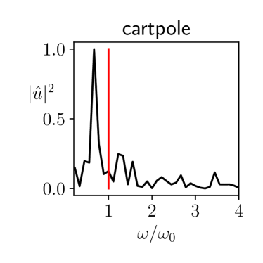
The temporal coherence of the inputs generated by FLEX is illustrated by Figure 5. The spectral density shows that the energy is peaked on a frequency, hence implying that there is a temporal structure exciting the cartole near resonance, and thereby yielding informative trajectories.
C.1.2 Environments
We provide additional details on the environments and the learning models used. We denote the translation variables by and and the angle variables by .
Environment 1 (Pendulum, ).
The dynamics are given by (2.5).
Environment 2 (Quadrotor, , ).
The planar quadrotor with nonlinear friction follows the following equations (Zhang et al., 2014)
| (C.1) | ||||
with the mass and the moment of inertia.
Environment 3 (Cartpole, ).
We implement the dynamics provided in (Barto et al., 1983).
Environment 4 (Robot arm / double pendulum, , ).
Equations available in (Chen, 2008).[, ]
C.1.3 Baselines
The random baselines returns . The uniform policy maximizes the uniformity objective by gradient descent, with 100 gradient steps at each time step. The periodic policy returns inputs of the for , with an eigenmode of the system.
C.1.4 Models
We use the following learning models in Section 6.1. of width 8 with one hidden layer and nonlinearity trained using ADAM optimizer (Kingma & Ba, 2015) with a batch size of 100.
Pendulum
We use the linear model of Example 2.1 and learn it by ordinary least squares.
Quadrotor
We learn the friction force with a neural net, and a learning rate of .
Cartpole
We parametrize with the observations , and and given by a neural network, trained with a learning rate of .
Arm
We use a neural network to learn as a function of and a learning rate of .
C.2 Tracking of time-varying dynamics
The state of the spaceship in the plane is denoted . The center of the star has time-varying coordinates
| (C.2) |
and the dynamics take the form
| (C.3) |
The agents know the dynamics down to the parameters and , which they learn by online gradient descent, with optimier ADAM and a learning rate of .
C.3 From exploration to exploitation

We add noise in the dynamics: for the pendulum and for the cartpole.
We use a linear model for the pendulum, and a neural network model with the same architecture as those of Section C.1 for the cartpole. The dynamics are learned as a function of and , and and for the cartpole.
Since we implemented our models with Pytorch (Paszke et al., 2017), we used we use the mpc package and the iLQR algorithm for exploitation (Amos et al., 2018). The quadratic costs are
| (C.4) |
for the pendulum and
| (C.5) |
for the cartpole. When comparing the cost values to competitors, only the order of magnitude matters since the control algorithm used for exploitation are different from an experiments to another.
We measured the computational time on a laptop and averaged it over 100 runs for FLEX and the random policy, then compared with the values of (Schultheis et al., 2020) and by setting the commputational time of the random policy to 1. Here again, only the orders of magnitude matter.
Appendix D Proofs
D.1 Proof of Proposition 1
Proof.
The data-generating distribution knowing the parameter can be computed using the probability chain rule:
| (D.1) |
which yields (omitting constants with respect to )
| (D.2) | ||||
Differentiating twice yields and taking the opposite yields
| (D.3) | ||||
∎
D.2 Proof of Proposition 2
D.3 Proof of Proposition 3
Proof.
See (Blanke & Lelarge, 2022). Since exploration aims at producing trajectories of large amplitude, we focus on inputs with maximal norm and assume an equality constraint in the optimization problem. The strict inequality can be handled readily with unconstrained minimization. Let us denote by a minimizer of (4.5), the eigenvalues of , and and the coordinates of and in a corresponding orthonormal basis. By the Lagrange multiplier theorem, there exists a nonzero scalar such that , where can be scaled such that is nonsingular. The inversion of the optimal condition and the expansion of the equality constraint yield
| (D.6a) | |||
| (D.6b) | |||
The minimizer is determined by solving (D.6b) for . ∎