This paper was converted on www.awesomepapers.org from LaTeX by an anonymous user.
Want to know more? Visit the Converter page.

\typearea

15

Floer cohomologies of non-torus fibers
of the Gelfand-Cetlin system

Yuichi Nohara and Kazushi Ueda
Abstract

The Gelfand-Cetlin system has non-torus Lagrangian fibers on some of the boundary strata of the moment polytope. We compute Floer cohomologies of such non-torus Lagrangian fibers in the cases of the 3-dimensional full flag manifold and the Grassmannian of 2-planes in a 4-space.

1 Introduction

Let PP be a parabolic subgroup of GL(n,)\operatorname{GL}(n,\mathbb{C}) and F:=GL(n,)/PF:=\operatorname{GL}(n,\mathbb{C})/P be the associated flag manifold. The Gelfand-Cetlin system, introduced by Guillemin and Sternberg [GS83], is a completely integrable system

Φ:F(dimF)/2,\Phi:F\longrightarrow\mathbb{R}^{(\dim_{\mathbb{R}}F)/2},

i.e., a set of functionally independent and Poisson commuting functions. The image Δ=Φ(F)\Delta=\Phi(F) is a convex polytope called the Gelfand-Cetlin polytope, and Φ\Phi gives a Lagrangian torus fibration structure over the interior IntΔ\operatorname{Int}\Delta of Δ\Delta. Unlike the case of toric manifolds where the fibers over the relative interior of a dd-dimensional face of the moment polytope are dd-dimensional isotropic tori, the Gelfand-Cetlin system has non-torus Lagrangian fibers over the relative interiors of some of the faces of Δ\Delta.

Let (X,ω)(X,\omega) be a compact toric manifold of dimX=N\dim_{\mathbb{C}}X=N, and Φ:XN\Phi:X\to\mathbb{R}^{N} be the toric moment map with the moment polytope Δ=Φ(X)\Delta=\Phi(X). For an interior point 𝒖IntΔ{\boldsymbol{u}}\in\operatorname{Int}\Delta, let L(𝒖)L({\boldsymbol{u}}) denote the Lagrangian torus fiber Φ1(𝒖)\Phi^{-1}({\boldsymbol{u}}). Lagrangian intersection Floer theory endows the cohomology group H(L(𝒖);Λ0)H^{*}(L({\boldsymbol{u}});\Lambda_{0}) over the Novikov ring

Λ0:={i=1aiTλi|ai,λi0,limiλi=}\Lambda_{0}:=\left\{\left.\sum_{i=1}^{\infty}a_{i}T^{\lambda_{i}}\,\right|\,a_{i}\in\mathbb{C},\ \lambda_{i}\geq 0,\ \lim_{i\to\infty}\lambda_{i}=\infty\right\}

with a structure {𝔪k}k0\{\mathfrak{m}_{k}\}_{k\geq 0} of a unital filtered AA_{\infty}-algebra [FOOO09]. Let Λ\Lambda and Λ+\Lambda_{+} be the quotient field and the maximal ideal of the local ring Λ0\Lambda_{0} respectively. An odd-degree element bHodd(L(𝒖);Λ0)b\in H^{\mathrm{odd}}(L({\boldsymbol{u}});\Lambda_{0}) is said to be a bounding cochain if it satisfies the Maurer-Cartan equation

k=0𝔪k(bk)=0.\sum_{k=0}^{\infty}\mathfrak{m}_{k}(b^{\otimes k})=0. (1.1)

A solution bHodd(L(𝒖);Λ0)b\in H^{\mathrm{odd}}(L({\boldsymbol{u}});\Lambda_{0}) to the weak Maurer-Cartan equation

k=0𝔪k(bk)0modΛ0𝐞0\displaystyle\sum_{k=0}^{\infty}\mathfrak{m}_{k}(b^{\otimes k})\equiv 0\mod\Lambda_{0}\,\mathbf{e}_{0} (1.2)

is called a weak bounding cochain, where 𝐞0\mathbf{e}_{0} is the unit in H(L(𝒖);Λ0)H^{*}(L({\boldsymbol{u}});\Lambda_{0}). The set of weak bounding cochains will be denoted by ^weak(L(𝒖))\widehat{\mathcal{M}}_{\mathrm{weak}}(L({\boldsymbol{u}})). The potential function is a map 𝔓𝔒:^weak(L(𝒖))Λ0\mathfrak{PO}\colon\widehat{\mathcal{M}}_{\mathrm{weak}}(L({\boldsymbol{u}}))\to\Lambda_{0} defined by

k=0𝔪k(b,,b)=𝔓𝔒(b)𝐞0.\displaystyle\sum_{k=0}^{\infty}\mathfrak{m}_{k}(b,\ldots,b)=\mathfrak{PO}(b)\mathbf{e}_{0}. (1.3)

A weak bounding cochain gives a deformed filtered AA_{\infty}-algebra whose AA_{\infty}-operations are given by

𝔪kb(x1,,xk)=m0=0mk=0𝔪m0++mk+k(bm0x1bm1xkbmk).\displaystyle\mathfrak{m}^{b}_{k}(x_{1},\ldots,x_{k})=\sum_{m_{0}=0}^{\infty}\cdots\sum_{m_{k}=0}^{\infty}\mathfrak{m}_{m_{0}+\cdots+m_{k}+k}(b^{\otimes m_{0}}\otimes x_{1}\otimes b^{\otimes m_{1}}\otimes\cdots\otimes x_{k}\otimes b^{\otimes m_{k}}). (1.4)

The weak Maurer-Cartan equation implies that 𝔪1b\mathfrak{m}_{1}^{b} squares to zero, and the deformed Floer cohomology is defined by

HF((L(𝒖),b),(L(𝒖),b);Λ0)=Ker(𝔪1b)/Im(𝔪1b).\displaystyle\mathop{H\!F}\nolimits((L({\boldsymbol{u}}),b),(L({\boldsymbol{u}}),b);\Lambda_{0})=\left.\operatorname{Ker}(\mathfrak{m}_{1}^{b})\right/\operatorname{Im}(\mathfrak{m}_{1}^{b}). (1.5)

More generally, one can deform the Floer differential 𝔪1\mathfrak{m}_{1} by

δb0,b1(x)=k0,k10𝔪k0+k1+1(b0,,b0k0,x,b1,,b1k1)\delta_{b_{0},b_{1}}(x)=\sum_{k_{0},k_{1}\geq 0}\mathfrak{m}_{k_{0}+k_{1}+1}(\underbrace{b_{0},\dots,b_{0}}_{k_{0}},x,\underbrace{b_{1},\dots,b_{1}}_{k_{1}}) (1.6)

for a pair (b0,b1)(b_{0},b_{1}) of weak bounding cochains with 𝔓𝔒(b0)=𝔓𝔒(b1)\mathfrak{PO}(b_{0})=\mathfrak{PO}(b_{1}). The Floer cohomology of the pair ((L(𝒖),b0),(L(𝒖),b1))((L({\boldsymbol{u}}),b_{0}),(L({\boldsymbol{u}}),b_{1})) is defined by

HF((L(𝒖),b0),(L(𝒖),b1);Λ0)=Ker(δb0,b1)/Im(δb0,b1).\displaystyle\mathop{H\!F}\nolimits((L({\boldsymbol{u}}),b_{0}),(L({\boldsymbol{u}}),b_{1});\Lambda_{0})=\left.\operatorname{Ker}(\delta_{b_{0},b_{1}})\right/\operatorname{Im}(\delta_{b_{0},b_{1}}). (1.7)

If the toric manifold XX is Fano, then the following hold [FOOO10]:

  • H1(L(𝒖);Λ0)H^{1}(L({\boldsymbol{u}});\Lambda_{0}) is contained in ^weak(L(𝒖))\widehat{\mathcal{M}}_{\mathrm{weak}}(L({\boldsymbol{u}})).

  • The potential function 𝔓𝔒\mathfrak{PO} on

    𝒖IntΔH1(L(𝒖);Λ0/2π1)IntΔ×(Λ0/2π1)N\bigcup_{{\boldsymbol{u}}\in\operatorname{Int}\Delta}H^{1}(L({\boldsymbol{u}});\Lambda_{0}/2\pi\sqrt{-1}\mathbb{Z})\cong\operatorname{Int}\Delta\times(\Lambda_{0}/2\pi\sqrt{-1}\mathbb{Z})^{N} (1.8)

    can be considered as a Laurent polynomial, which can be identified with the superpotential of the Landau-Ginzburg mirror of XX.

  • Each critical point of 𝔓𝔒\mathfrak{PO} corresponds to a pair (𝒖,b)({\boldsymbol{u}},b) such that the deformed Floer cohomology HF((L(𝒖),b),(L(𝒖),b);Λ)\mathop{H\!F}\nolimits((L({\boldsymbol{u}}),b),(L({\boldsymbol{u}}),b);\Lambda) over the Novikov field Λ\Lambda is non-trivial.

  • If the deformed Floer cohomology group over the Novikov field is non-trivial, then it is isomorphic to the classical cohomology group;

    HF((L(𝒖),b),(L(𝒖),b);Λ)H(TN;Λ).\displaystyle\mathop{H\!F}\nolimits((L({\boldsymbol{u}}),b),(L({\boldsymbol{u}}),b);\Lambda)\cong H^{*}(T^{N};\Lambda). (1.9)
  • The quantum cohomology ring QH(X;Λ)\mathop{QH}\nolimits(X;\Lambda) is isomorphic to the Jacobi ring Jac(𝔓𝔒)\operatorname{Jac}(\mathfrak{PO}) of the potential function.

In particular, the number of pairs (L(𝒖),b)(L({\boldsymbol{u}}),b) with nontrivial Floer cohomology coincides with rankQH(X;Λ)=rankH(X;Λ).\operatorname{rank}\mathop{QH}\nolimits(X;\Lambda)=\operatorname{rank}H^{*}(X;\Lambda).

Nishinou and the authors [NNU10] introduced the notion of a toric degeneration of an integrable system, and used it to compute the potential function of Lagrangian torus fibers of the Gelfand-Cetlin system. The resulting potential function can be considered as a Laurent polynomial just as in the toric Fano case, which can be identified with the superpotential of the Landau-Ginzburg mirror of the flag manifold given in [Giv97, BCFKvS00]. In contrast to the toric case, the rank of H(F;Λ)H^{*}(F;\Lambda) is greater in general than the rank of the Jacobi ring Jac(𝔓𝔒)\operatorname{Jac}(\mathfrak{PO}), and hence than the number of Lagrangian torus fibers with non-trivial Floer cohomology. In the case of the 3-dimensional flag manifold Fl(3)\operatorname{Fl}(3), the potential function has six critical points, which is equal to the rank of H(Fl(3);Λ)H^{*}(\operatorname{Fl}(3);\Lambda). Similarly, the potential function for the Grassmannian Gr(2,5)\operatorname{Gr}(2,5) of 2-planes in 5\mathbb{C}^{5} has ten critical points, which is equal to the rank of H(Gr(2,5);Λ)H^{*}(\operatorname{Gr}(2,5);\Lambda). On the other hand, the number of critical points of the potential function for the Grassmannian Gr(2,4)\operatorname{Gr}(2,4) of 2-planes in 4\mathbb{C}^{4} is four, which is less than the rank of H(Gr(2,4);Λ)H^{*}(\operatorname{Gr}(2,4);\Lambda), which is six.

In this paper, we study non-torus Lagrangian fibers of the Gelfand-Cetlin system over the boundary of the Gelfand-Cetlin polytope in the cases of Fl(3)\operatorname{Fl}(3) and Gr(2,4)\operatorname{Gr}(2,4). The main results are the following:

Theorem 1.1.

Let Φ:Fl(3)3\Phi\colon\operatorname{Fl}(3)\to\mathbb{R}^{3} be the Gelfand-Cetlin system with the Gelfand-Cetlin polytope Δ=Φ(Fl(3))\Delta=\Phi(\operatorname{Fl}(3)).

  1. 1.

    There exists a vertex 𝒖0{\boldsymbol{u}}_{0} of Δ\Delta such that a fiber L(𝒖)=Φ1(𝒖)L({\boldsymbol{u}})=\Phi^{-1}({\boldsymbol{u}}) over a boundary point 𝒖Δ{\boldsymbol{u}}\in\partial\Delta is a Lagrangian submanifold if and only if 𝒖=𝒖0{\boldsymbol{u}}={\boldsymbol{u}}_{0}.

  2. 2.

    The Lagrangian fiber L(𝒖0)L({\boldsymbol{u}}_{0}) is diffeomorphic to SU(2)S3\operatorname{SU}(2)\cong S^{3}.

  3. 3.

    The Floer cohomology of L(𝒖0)L({\boldsymbol{u}}_{0}) over the Novikov field Λ\Lambda is trivial;

    HF(L(𝒖0),L(𝒖0);Λ)=0.\mathop{H\!F}\nolimits(L({\boldsymbol{u}}_{0}),L({\boldsymbol{u}}_{0});\Lambda)=0. (1.10)
Theorem 1.2.

Let Φ:Gr(2,4)4\Phi\colon\operatorname{Gr}(2,4)\to\mathbb{R}^{4} be the Gelfand-Cetlin system with the Gelfand-Cetlin polytope Δ=Φ(Gr(2,4))\Delta=\Phi(\operatorname{Gr}(2,4)).

  1. 1.

    There exists an edge of Δ\Delta such that a fiber L(𝒖)=Φ1(𝒖)L({\boldsymbol{u}})=\Phi^{-1}({\boldsymbol{u}}) over 𝒖Δ{\boldsymbol{u}}\in\partial\Delta is a Lagrangian submanifold if and only if 𝒖{\boldsymbol{u}} is in the relative interior of the edge.

  2. 2.

    The Lagrangian fiber L(𝒖)L({\boldsymbol{u}}) over any point 𝒖{\boldsymbol{u}} in the relative interior of the edge is diffeomorphic to U(2)S1×S3\operatorname{U}(2)\cong S^{1}\times S^{3}.

  3. 3.

    H1(L(𝒖);Λ0)H^{1}(L({\boldsymbol{u}});\Lambda_{0}) is contained in ^weak(L(𝒖))\widehat{\mathcal{M}}_{\mathrm{weak}}(L({\boldsymbol{u}})).

  4. 4.

    The potential function is identically zero on H1(L(𝒖);Λ0)H^{1}(L({\boldsymbol{u}});\Lambda_{0}).

  5. 5.

    The Floer cohomology HF((L(𝒖),b),(L(𝒖),b);Λ)\mathop{H\!F}\nolimits((L({\boldsymbol{u}}),b),(L({\boldsymbol{u}}),b);\Lambda) of a Lagrangian U(2)\operatorname{U}(2)-fiber L(𝒖)L({\boldsymbol{u}}) over the Novikov field Λ\Lambda is non-trivial if and only if 𝒖{\boldsymbol{u}} is the barycenter 𝒖0{\boldsymbol{u}}_{0} of the edge and b=±π1/2𝐞1b=\pm\pi\sqrt{-1}/2\,\mathbf{e}_{1}, where 𝐞1\mathbf{e}_{1} is a generator of H1(L(𝒖);)H^{1}(L({\boldsymbol{u}});\mathbb{Z})\cong\mathbb{Z}.

  6. 6.

    If the deformed Floer cohomology group over the Novikov field is non-trivial, then it is isomorphic to the classical cohomology group;

    HF((L(𝒖0),±π1/2𝐞1),(L(𝒖0),±π1/2𝐞1);Λ)H(S1×S3;Λ).\displaystyle\mathop{H\!F}\nolimits((L({\boldsymbol{u}}_{0}),\pm\pi\sqrt{-1}/2\,\mathbf{e}_{1}),(L({\boldsymbol{u}}_{0}),\pm\pi\sqrt{-1}/2\,\mathbf{e}_{1});\Lambda)\cong H^{*}(S^{1}\times S^{3};\Lambda). (1.11)
  7. 7.

    The Floer cohomology of the pair ((L(𝒖0),π1/2𝐞1),(L(𝒖0),π1/2𝐞1))((L({\boldsymbol{u}}_{0}),\pi\sqrt{-1}/2\,\mathbf{e}_{1}),(L({\boldsymbol{u}}_{0}),-\pi\sqrt{-1}/2\,\mathbf{e}_{1})) is trivial;

    HF((L(𝒖0),π1/2𝐞1),(L(𝒖0),π1/2𝐞1);Λ)=0.\displaystyle\mathop{H\!F}\nolimits((L({\boldsymbol{u}}_{0}),\pi\sqrt{-1}/2\,\mathbf{e}_{1}),(L({\boldsymbol{u}}_{0}),\pi\sqrt{-1}/2\,\mathbf{e}_{1});\Lambda)=0. (1.12)

More precise statements, which describe the Floer cohomology groups over the Novikov ring Λ0\Lambda_{0}, are given in Theorem 4.8, Theorem 4.16, and Theorem 4.20.

A symplectic manifold (X,ω)(X,\omega) is monotone if the cohomology class [ω][\omega] is positively proportional to the first Chern class;

λ>0[ω]=λc1(X).\displaystyle\exists\lambda>0\quad[\omega]=\lambda c_{1}(X). (1.13)

The quantum cohomology ring of a monotone symplectic manifold does not have any convergence issue, and hence is defined over \mathbb{C}. A Lagrangian submanifold LL is monotone if the symplectic area of a disk bounded by LL is positively proportional to the Maslov index;

λ>0βπ2(M,L)βω=λμ(β).\displaystyle\exists\lambda>0\quad\forall\beta\in\pi_{2}(M,L)\quad\beta\cap\omega=\lambda\mu(\beta). (1.14)

The AA_{\infty}-operations on the Lagrangian intersection Floer complex of a monotone Lagrangian submanifold is defined over \mathbb{C}. The minimal Maslov number of oriented monotone Lagrangian submanifold is greater than or equal to 2, so that the obstruction class 𝔪0(1)\mathfrak{m}_{0}(1) can be written as 𝔪0(1)=𝔪0(L)𝐞0,\mathfrak{m}_{0}(1)=\mathfrak{m}_{0}(L)\,\mathbf{e}_{0}, where 𝔪0(L)\mathfrak{m}_{0}(L)\in\mathbb{C} is the count of Maslov index 2 disks bounded by LL, weighted by their symplectic areas and holonomies of a flat U(1)U(1)-bundle on LL along the boundaries of the disks. The monotone Fukaya category is defined as the direct sum

(X):=λ(X;λ),\displaystyle\mathcal{F}(X):=\bigoplus_{\lambda\in\mathbb{C}}\mathcal{F}(X;\lambda), (1.15)

where (X;λ)\mathcal{F}(X;\lambda) is an AA_{\infty}-category over \mathbb{C} whose objects are monotone Lagrangian submanifolds, equipped with flat U(1)U(1)-bundles, satisfying 𝔪0(L)=λ\mathfrak{m}_{0}(L)=\lambda. For any monotone Lagrangian submanifold LL, there is a natural ring homomorphism

QH(X)HF(L,L),\displaystyle\mathop{QH}\nolimits(X)\to\mathop{H\!F}\nolimits(L,L), (1.16)

which is known by Auroux [Aur07], Kontsevich, and Seidel to send c1(X)QH(X)c_{1}(X)\in\mathop{QH}\nolimits(X) to 𝔪0(1)HF(L,L)\mathfrak{m}_{0}(1)\in\mathop{H\!F}\nolimits(L,L). It follows that (X;λ)\mathcal{F}(X;\lambda) is trivial unless λ\lambda is an eigenvalue of the quantum cup product by c1(X)c_{1}(X).

Now consider the case when X=Gr(2,4)X=\operatorname{Gr}(2,4), which can be written as a quadric hypersurface

X={[z0::z5]5|z02=z12++z52}.\displaystyle X=\left\{[z_{0}:\cdots:z_{5}]\in\mathbb{P}^{5}\mathrel{}\middle|\mathrel{}z_{0}^{2}=z_{1}^{2}+\cdots+z_{5}^{2}\right\}. (1.17)

The real locus XX_{\mathbb{R}} is a monotone Lagrangian sphere, which is the vanishing cycle along a degeneration into a nodal quadric and split-generates the nilpotent summand Dπ(X;0)D^{\pi}\mathcal{F}(X;0) of the monotone Fukaya category [Smi12, Lemma 4.6]. The Floer cohomology HF(X,X)\mathop{H\!F}\nolimits(X_{\mathbb{R}},X_{\mathbb{R}}) is semisimple, and carries a formal AA_{\infty}-structure [Smi12, Lemma 4.7]. It follows that Dπ(X;0)D^{\pi}\mathcal{F}(X;0) is equivalent to the direct sum of two copies of the derived category Db()D^{b}(\mathbb{C}) of \mathbb{C}-vector spaces. On the other hand, (L(𝒖0),±π1/2𝐞1)(L({\boldsymbol{u}}_{0}),\pm\pi\sqrt{-1}/2\,\mathbf{e}_{1}) are also objects of the nilpotent summand Dπ(X;0)D^{\pi}\mathcal{F}(X;0) of the monotone Fukaya category, which are non-zero by (1.11). Since (L(𝒖0),±1/2𝐞1)(L({\boldsymbol{u}}_{0}),\pm\sqrt{-1}/2\,\mathbf{e}_{1}) is a pair of orthogonal non-zero objects in a triangulated category equivalent to Db()Db()D^{b}(\mathbb{C})\oplus D^{b}(\mathbb{C}), they split-generate the whole category:

Corollary 1.3.

The pair (L(𝐮0),±π1/2𝐞1)(L({\boldsymbol{u}}_{0}),\pm\pi\sqrt{-1}/2\,\mathbf{e}_{1}) split-generate Dπ(Gr(2,4);0)D^{\pi}\mathcal{F}(\operatorname{Gr}(2,4);0).

Acknowledgment: We thank Hiroshi Ohta, Kaoru Ono, and Yoshihiro Ohnita for useful conversations. Y. N. is supported by Grant-in-Aid for Young Scientists (No.23740055). K. U. is supported by Grant-in-Aid for Young Scientists (No.24740043).

2 Non-torus fibers of the Gelfand-Cetlin system

2.1 Flag manifolds

For a sequence 0=n0<n1<<nr<nr+1=n0=n_{0}<n_{1}<\dots<n_{r}<n_{r+1}=n of integers, let F=F(n1,,nr,n)F=F(n_{1},\dots,n_{r},n) be the flag manifold consisting of flags

0V1Vrn,dimVi=ni0\subset V_{1}\subset\dots\subset V_{r}\subset\mathbb{C}^{n},\quad\dim V_{i}=n_{i}

of n\mathbb{C}^{n}. We write the full flag manifold and the Grassmannian as Fl(n)=F(1,2,,n)\operatorname{Fl}(n)=F(1,2,\dots,n) and Gr(k,n)=F(k,n)\operatorname{Gr}(k,n)=F(k,n) respectively. The complex dimension of F(n1,,nr,n)F(n_{1},\dots,n_{r},n) is given by

N=N(n1,,nr,n):=dimF(n1,,nr,n)=i=1r(nini1)(nni).N=N(n_{1},\dots,n_{r},n):=\dim_{\mathbb{C}}F(n_{1},\dots,n_{r},n)=\sum_{i=1}^{r}(n_{i}-n_{i-1})(n-n_{i}).

Let P=P(n1,,nr,n)GL(n,)P=P(n_{1},\dots,n_{r},n)\subset\operatorname{GL}(n,\mathbb{C}) be the stabilizer subgroup of the standard flag (Vi=e1,,eni)i=1r,(V_{i}=\langle e_{1},\dots,e_{n_{i}}\rangle)_{i=1}^{r}, where {ei}i=1n\{e_{i}\}_{i=1}^{n} is the standard basis of n\mathbb{C}^{n}. The intersection of PP and U(n)\operatorname{U}(n) is U(k1)××U(kr+1)\operatorname{U}(k_{1})\times\dots\times\operatorname{U}(k_{r+1}) for ki=nini1k_{i}=n_{i}-n_{i-1}, and FF is written as

F=GL(n,)/P=U(n)/(U(k1)××U(kr+1)).F=\operatorname{GL}(n,\mathbb{C})/P=\operatorname{U}(n)/(\operatorname{U}(k_{1})\times\dots\times\operatorname{U}(k_{r+1})).

We take a U(n)\operatorname{U}(n)-invariant inner product x,y=trxy\langle x,y\rangle=\operatorname{tr}xy^{*} on the Lie algebra 𝔲(n)\mathfrak{u}(n) of U(n)\operatorname{U}(n), and identify the dual vector space 𝔲(n)\mathfrak{u}(n)^{*} of 𝔲(n)\mathfrak{u}(n) with the space 1𝔲(n)\sqrt{-1}\mathfrak{u}(n) of Hermitian matrices. For 𝝀=diag(λ1,,λn)1𝔲(n){\boldsymbol{\lambda}}=\mathrm{diag}\,(\lambda_{1},\dots,\lambda_{n})\in\sqrt{-1}\mathfrak{u}(n) with

λ1==λn1k1>λn1+1==λn2k2>>λnr+1==λnkr+1,\underbrace{\lambda_{1}=\dots=\lambda_{n_{1}}}_{k_{1}}>\underbrace{\lambda_{n_{1}+1}=\dots=\lambda_{n_{2}}}_{k_{2}}>\dots>\underbrace{\lambda_{n_{r}+1}=\dots=\lambda_{n}}_{k_{r+1}}, (2.1)

the flag manifold FF is identified with the adjoint orbit 𝒪𝝀1𝔲(n)\mathcal{O}_{{\boldsymbol{\lambda}}}\subset\sqrt{-1}\mathfrak{u}(n) of 𝝀{\boldsymbol{\lambda}}. Note that 𝒪𝝀\mathcal{O}_{{\boldsymbol{\lambda}}} consists of Hermitian matrices with fixed eigenvalues λ1,,λn\lambda_{1},\dots,\lambda_{n}. Let

ω(adξ(x),adη(x))=12πx,[ξ,η],ξ,η𝔲(n)\omega(\operatorname{ad}_{\xi}(x),\operatorname{ad}_{\eta}(x))=\frac{1}{2\pi}\langle x,[\xi,\eta]\rangle,\quad\xi,\eta\in\mathfrak{u}(n)

be the (normalized) Kostant-Kirillov form on 𝒪𝝀\mathcal{O}_{{\boldsymbol{\lambda}}}.

For each i=1,,ri=1,\dots,r, we set i:=(nin)(nni)1\mathbb{P}_{i}:=\mathbb{P}\bigl{(}\bigwedge^{n_{i}}\mathbb{C}^{n}\bigr{)}\cong\mathbb{P}^{\binom{n}{n_{i}}-1}. Then the Plücker embedding is given by

ι:Fi=1ri,(0V1Vrn)(n1V1,,nrVr).\iota:F\hookrightarrow\prod_{i=1}^{r}\mathbb{P}_{i},\quad(0\subset V_{1}\subset\dots\subset V_{r}\subset\mathbb{C}^{n})\mapsto(\textstyle{\bigwedge^{n_{1}}}V_{1},\dots,\textstyle{\bigwedge^{n_{r}}}V_{r}).

Let ωi\omega_{\mathbb{P}_{i}} be the Fubini-Study form on i\mathbb{P}_{i} normalized in such a way that it represents the first Chern class c1(𝒪(1))c_{1}(\mathcal{O}(1)) of the hyperplane bundle. Then the Kostant-Kirillov form ω\omega and the first Chern form c1(F)c_{1}(F) of FF are given by

ω\displaystyle\omega =i=1r(λniλni+1)ωi\displaystyle=\sum_{i=1}^{r}(\lambda_{n_{i}}-\lambda_{n_{i+1}})\omega_{\mathbb{P}_{i}}

and

c1(F)\displaystyle c_{1}(F) =i=1r(ni+1ni1)ωi\displaystyle=\sum_{i=1}^{r}(n_{i+1}-n_{i-1})\omega_{\mathbb{P}_{i}}

respectively.

Example 2.1.

The 3-dimensional full flag manifold Fl(3)\operatorname{Fl}(3) is embedded into

1×2=(3)×(23)2×2\mathbb{P}_{1}\times\mathbb{P}_{2}=\mathbb{P}(\mathbb{C}^{3})\times\mathbb{P}(\textstyle{\bigwedge^{2}\mathbb{C}^{3}})\cong\mathbb{P}^{2}\times\mathbb{P}^{2}

as a hypersurface. The image of Fl(3)\operatorname{Fl}(3) is given by the Plücker relation

Z1Z23+Z2Z31+Z3Z12=0,Z_{1}Z_{23}+Z_{2}Z_{31}+Z_{3}Z_{12}=0,

where [Z1:Z2:Z3][Z_{1}:Z_{2}:Z_{3}] and [Z23:Z31:Z12][Z_{23}:Z_{31}:Z_{12}] are the Plücker coordinates on 1\mathbb{P}_{1} and 2\mathbb{P}_{2} respectively.

Example 2.2.

The Grassmannian Gr(2,4)\operatorname{Gr}(2,4) of 2-plans in 4\mathbb{C}^{4} is embedded into (24)5\mathbb{P}(\bigwedge^{2}\mathbb{C}^{4})\cong\mathbb{P}^{5} as a hypersurface. The Plücker relation is given by

Z12Z34Z13Z24+Z14Z23=0,Z_{12}Z_{34}-Z_{13}Z_{24}+Z_{14}Z_{23}=0,

where [Z12:Z13:Z14:Z23:Z24:Z34][Z_{12}:Z_{13}:Z_{14}:Z_{23}:Z_{24}:Z_{34}] is the Plücker coordinates.

2.2 The Gelfand-Cetlin system

For x𝒪𝝀x\in\mathcal{O}_{{\boldsymbol{\lambda}}} and k=1,,n1k=1,\dots,n-1, let x(k)x^{(k)} denote the upper-left k×kk\times k submatrix of xx. Since x(k)x^{(k)} is also a Hermitian matrix, it has real eigenvalues λ1(k)(x)λ2(k)(x)λk(k)(x)\lambda^{(k)}_{1}(x)\geq\lambda^{(k)}_{2}(x)\geq\dots\geq\lambda^{(k)}_{k}(x). By taking the eigenvalues for all k=1,,n1k=1,\dots,n-1, we obtain a set (λi(k))1ikn1(\lambda^{(k)}_{i})_{1\leq i\leq k\leq n-1} of n(n1)/2n(n-1)/2 functions, which satisfy the inequalities

λ1λ2λ3λn1λnλ1(n1)λ2(n1)λn1(n1)λ1(n2)λn2(n2)λ1(1).\begin{aligned} \hbox to16.49995pt{$\hfill\lambda_{1}\hfill$}&&&&\hbox to16.49995pt{$\hfill\lambda_{2}\hfill$}&&&&\hbox to16.49995pt{$\hfill\lambda_{3}\hfill$}&&\cdots&&\hbox to16.49995pt{$\hfill\lambda_{n-1}\hfill$}&&&&\hbox to16.49995pt{$\hfill\lambda_{n}\hfill$}\\ &\rotatebox[origin={c}]{315.0}{$\geq$}&&\rotatebox[origin={c}]{45.0}{$\geq$}&&\rotatebox[origin={c}]{315.0}{$\geq$}&&\rotatebox[origin={c}]{45.0}{$\geq$}&&&&&&\rotatebox[origin={c}]{315.0}{$\geq$}&&\rotatebox[origin={c}]{45.0}{$\geq$}&\\ &&\hbox to16.49995pt{$\lambda_{1}^{(n-1)}$}&&&&\hbox to16.49995pt{$\lambda_{2}^{(n-1)}$}&&&&&&&&\hbox to16.49995pt{$\lambda_{n-1}^{(n-1)}$}&&\\ &&&\rotatebox[origin={c}]{315.0}{$\geq$}&&\rotatebox[origin={c}]{45.0}{$\geq$}&&&&&&&&\rotatebox[origin={c}]{45.0}{$\geq$}&&&\\ &&&&\hbox to16.49995pt{$\lambda_{1}^{(n-2)}$}&&&&&&&&\hbox to16.49995pt{$\lambda_{n-2}^{(n-2)}$}&&&&\\ &&&&&\rotatebox[origin={c}]{315.0}{$\geq$}&&&&&&\rotatebox[origin={c}]{45.0}{$\geq$}&&&&&\\ &&&&&&\rotatebox[origin={c}]{315.0}{$\cdots$}&&&&\rotatebox[origin={c}]{45.0}{$\cdots$}&&&&&&\\ &&&&&&&\rotatebox[origin={c}]{315.0}{$\geq$}&&\rotatebox[origin={c}]{45.0}{$\geq$}&&&&&&&\\ &&&&&&&&\hbox to16.49995pt{$\lambda_{1}^{(1)}$}&&&&&&&&&\end{aligned}. (2.2)

It follows that the number of non-constant λi(k)\lambda^{(k)}_{i} coincides with N=dimFN=\dim_{\mathbb{C}}F. Let I=I(n1,,nr,n)I=I(n_{1},\dots,n_{r},n) denotes the set of pairs (i,k)(i,k) such that λi(k)\lambda_{i}^{(k)} is non-constant. Then the Gelfand-Cetlin system is defined by

Φ=(λi(k))(i,k)I:F(n1,,nr,n)N(n1,,nr,n).\Phi=(\lambda^{(k)}_{i})_{(i,k)\in I}:F(n_{1},\dots,n_{r},n)\longrightarrow\mathbb{R}^{N(n_{1},\dots,n_{r},n)}.
Proposition 2.3 (Guillemin and Sternberg [GS83]).

The map Φ\Phi is a completely integrable system on (F(n1,,nr,n),ω)(F(n_{1},\dots,n_{r},n),\omega). The functions λi(k)\lambda_{i}^{(k)} are action variables, and the image Δ=Φ(F)\Delta=\Phi(F) is a convex polytope defined by (2.2). The fiber L(𝐮)=Φ1(𝐮)L({\boldsymbol{u}})=\Phi^{-1}({\boldsymbol{u}}) over each interior point 𝐮IntΔ{\boldsymbol{u}}\in\operatorname{Int}\Delta is a Lagrangian torus.

The image ΔN(n1,,nr,n)\Delta\subset\mathbb{R}^{N(n_{1},\dots,n_{r},n)} is called the Gelfand-Cetlin polytope. The Gelfand-Cetlin system is not smooth on the locus where λk(i)=λk(i+1)\lambda_{k}^{(i)}=\lambda_{k}^{(i+1)} for some (i,k)(i,k), or equivalently, where the Gelfand-Cetlin pattern (2.2) contains a set of equalities of the form

λk+1(i+1)==λk(i)λk(i+1)==λk1(i).\begin{aligned} &&\hbox to16.49995pt{$\hfill{\lambda_{k+1}^{(i+1)}}\hfill$}&&\\ &\rotatebox[origin={c}]{45.0}{$=$}&&\rotatebox[origin={c}]{315.0}{$=$}&&\phantom{\rotatebox[origin={c}]{315.0}{$\geq$}}&\\ \hbox to16.49995pt{$\hfill{\lambda_{k}^{(i)}}\hfill$}&&&&\hbox to16.49995pt{$\hfill{\lambda_{k}^{(i+1)}}\hfill$}&&\\ &\rotatebox[origin={c}]{315.0}{$=$}&&\rotatebox[origin={c}]{45.0}{$=$}&&&\\ &&\hbox to16.49995pt{$\hfill{\lambda_{k-1}^{(i)}}\hfill$}&&&&\end{aligned}.

The image of such loci are faces of Δ\Delta of codimension greater than two where Δ\Delta does not satisfy the Delzant condition. Away from such faces, each fiber Φ1(𝒖)\Phi^{-1}({\boldsymbol{u}}) of Φ\Phi is an isotropic torus whose dimension is that of the face of Δ\Delta containing 𝒖{\boldsymbol{u}} in its relative interior.

2.3 The case of Fl(3)\operatorname{Fl}(3)

Refer to caption
Figure 2.1: The Gelfand-Cetlin polytope for Fl(3)\operatorname{Fl}(3)

After a translation by a scalar matrix, we may assume that Fl(3)\operatorname{Fl}(3) is identified with the adjoint orbit of 𝝀=diag(λ1,0,λ2){\boldsymbol{\lambda}}=\operatorname{diag}(\lambda_{1},0,-\lambda_{2}) for λ1,λ2>0\lambda_{1},\lambda_{2}>0. Then the Gelfand-Cetlin polytope Δ\Delta consists of (u1,u2,u3)3(u_{1},u_{2},u_{3})\in\mathbb{R}^{3} satisfying

λ1\displaystyle 0\displaystyle λ2\displaystyle (2.3)
\displaystyle\rotatebox[origin={c}]{315.0}{$\geq$} \displaystyle\rotatebox[origin={c}]{45.0}{$\geq$} \displaystyle\rotatebox[origin={c}]{315.0}{$\geq$} \displaystyle\rotatebox[origin={c}]{45.0}{$\geq$}
u1\displaystyle u2\displaystyle
\displaystyle\rotatebox[origin={c}]{315.0}{$\geq$} \displaystyle\rotatebox[origin={c}]{45.0}{$\geq$}
u3\displaystyle

as shown in Figure 2.1. The non-smooth locus of Φ\Phi is the fiber L0=Φ1(𝟎)L_{0}=\Phi^{-1}({\boldsymbol{0}}) over the vertex 𝟎=(0,0,0)Δ{\boldsymbol{0}}=(0,0,0)\in\Delta where four edges intersect.

Definition 2.4 (Evans and Lekili [EL, Definition 1.1.1]).

Let KK be a compact connected Lie group. A Lagrangian submanifold LL in a Kähler manifold XX is said to be KK-homogeneous if KK acts holomorphically on XX in such a way that LL is a KK-orbit.

Proposition 2.5.

The fiber L0=Φ1(𝟎)L_{0}=\Phi^{-1}({\boldsymbol{0}}) is a Lagrangian 3-sphere given by

L0={(00z100z2z¯1z¯2λ1λ2)1𝔲(3)||z1|2+|z2|2=λ1λ2},L_{0}=\left\{\left.\begin{pmatrix}0&0&z_{1}\\ 0&0&z_{2}\\ \overline{z}_{1}&\overline{z}_{2}&\lambda_{1}-\lambda_{2}\end{pmatrix}\in\sqrt{-1}\mathfrak{u}(3)\right||z_{1}|^{2}+|z_{2}|^{2}=\lambda_{1}\lambda_{2}\right\},

which is KK-homogeneous for

K={(a1a¯20a2a¯10001)||a1|2+|a2|2=1}SU(2).K=\left\{\left.\begin{pmatrix}a_{1}&-\overline{a}_{2}&0\\ a_{2}&\overline{a}_{1}&0\\ 0&0&1\end{pmatrix}\right||a_{1}|^{2}+|a_{2}|^{2}=1\right\}\cong\operatorname{SU}(2).
Proof.

Suppose that xL0x\in L_{0}. Then λ1(2)(x)=λ2(2)(x)=0\lambda_{1}^{(2)}(x)=\lambda_{2}^{(2)}(x)=0 implies that x(2)=0x^{(2)}=0 and thus xx has the form

x=(00z100z2z¯1z¯2x33)x=\begin{pmatrix}0&0&z_{1}\\ 0&0&z_{2}\\ \overline{z}_{1}&\overline{z}_{2}&x_{33}\end{pmatrix}

for some z1,z2z_{1},z_{2}\in\mathbb{C} and x33x_{33}\in\mathbb{R}. Since

det(λx)=λ(λ2x33λ(|z1|2+|z2|2))=0\operatorname{det}(\lambda-x)=\lambda\left(\lambda^{2}-x_{33}\lambda-(|z_{1}|^{2}+|z_{2}|^{2})\right)=0

has solutions λ=λ1,0,λ2\lambda=\lambda_{1},0,-\lambda_{2}, we have x33=λ1λ2x_{33}=\lambda_{1}-\lambda_{2} and |z1|2+|z2|2=λ1λ2|z_{1}|^{2}+|z_{2}|^{2}=\lambda_{1}\lambda_{2}. Hence the fiber L0L_{0} is the KK-orbit of

(00λ1λ2000λ1λ20λ1λ2)=Adg0(λ10000000λ2)𝒪𝝀,\begin{pmatrix}0&0&\sqrt{\lambda_{1}\lambda_{2}}\\ 0&0&0\\ \sqrt{\lambda_{1}\lambda_{2}}&0&\lambda_{1}-\lambda_{2}\end{pmatrix}=\operatorname{Ad}_{g_{0}}\begin{pmatrix}\lambda_{1}&0&0\\ 0&0&0\\ 0&0&-\lambda_{2}\end{pmatrix}\in\mathcal{O}_{{\boldsymbol{\lambda}}},

where

g0=(λ2/(λ1+λ2)0λ1/(λ1+λ2)010λ1/(λ1+λ2)0λ2/(λ1+λ2))SU(3).g_{0}=\begin{pmatrix}\sqrt{\lambda_{2}/(\lambda_{1}+\lambda_{2})}&0&-\sqrt{\lambda_{1}/(\lambda_{1}+\lambda_{2})}\\ 0&1&0\\ \sqrt{\lambda_{1}/(\lambda_{1}+\lambda_{2})}&0&\sqrt{\lambda_{2}/(\lambda_{1}+\lambda_{2})}\end{pmatrix}\in\operatorname{SU}(3).

Next we see that L0L_{0} is Lagrangian. Since KK acts transitively on L0L_{0}, the tangent space TxL0T_{x}L_{0} is spanned by infinitesimal actions adξ(x)\operatorname{ad}_{\xi}(x) of ξ𝔨\xi\in\mathfrak{k}, where

𝔨={ξ=(ξ(2)000)𝔲(3)|ξ(2)𝔰𝔲(2)}𝔰𝔲(2)\mathfrak{k}=\biggl{\{}\xi=\begin{pmatrix}\xi^{(2)}&0\\ 0&0\end{pmatrix}\in\mathfrak{u}(3)\biggm{|}\xi^{(2)}\in\mathfrak{su}(2)\biggr{\}}\cong\mathfrak{su}(2)

is the Lie algebra of KK. Since x(2)=0x^{(2)}=0 for xL0x\in L_{0}, we have

ω(adξ(x),adη(x))=12πtr(x(2)[ξ(2),η(2)])=0\omega(\operatorname{ad}_{\xi}(x),\operatorname{ad}_{\eta}(x))=\frac{\sqrt{-1}}{2\pi}\operatorname{tr}\Bigl{(}x^{(2)}[\xi^{(2)},\eta^{(2)}]\Bigr{)}=0

for any ξ,η𝔨\xi,\eta\in\mathfrak{k}. ∎

Let ι:Fl(3)1×2=(3)×(23)\iota:\operatorname{Fl}(3)\to\mathbb{P}_{1}\times\mathbb{P}_{2}=\mathbb{P}(\mathbb{C}^{3})\times\mathbb{P}(\bigwedge^{2}\mathbb{C}^{3}) be the Plücker embedding and ([Z1:Z2:Z3],[Z23:Z31:Z12])([Z_{1}:Z_{2}:Z_{3}],[Z_{23}:Z_{31}:Z_{12}]) be the Plücker coordinates. The Kostant-Kirillov form is given by

ω=λ1ω1+λ2ω2.\omega=\lambda_{1}\omega_{\mathbb{P}_{1}}+\lambda_{2}\omega_{\mathbb{P}_{2}}.

Since the Lagrangian fiber L0L_{0} as a submanifold in SU(3)/T\operatorname{SU}(3)/T consists of

(a1a¯20a2a¯10001)g0=1λ1+λ2(λ2a1λ1+λ2a¯2λ1a1λ2a2λ1+λ2a¯1λ1a2λ10λ2)modT\begin{pmatrix}a_{1}&-\overline{a}_{2}&0\\ a_{2}&\overline{a}_{1}&0\\ 0&0&1\end{pmatrix}g_{0}=\frac{1}{\sqrt{\lambda_{1}+\lambda_{2}}}\begin{pmatrix}\sqrt{\lambda_{2}}a_{1}&-\sqrt{\lambda_{1}+\lambda_{2}}\overline{a}_{2}&-\sqrt{\lambda_{1}}a_{1}\\ \sqrt{\lambda_{2}}a_{2}&\sqrt{\lambda_{1}+\lambda_{2}}\overline{a}_{1}&-\sqrt{\lambda_{1}}a_{2}\\ \sqrt{\lambda_{1}}&0&\sqrt{\lambda_{2}}\end{pmatrix}\mod T

with |a1|2+|a2|2=1|a_{1}|^{2}+|a_{2}|^{2}=1, the image ι(L0)\iota(L_{0}) is given by

ι(L0)={([a1:a2:λ1λ2],[a¯1:a¯2:λ2λ1])||a1|2+|a2|2=1}.\iota(L_{0})=\Biggl{\{}\Biggm{(}\left[a_{1}:a_{2}:\sqrt{\frac{\lambda_{1}}{\lambda_{2}}}\right],\left[\overline{a}_{1}:\overline{a}_{2}:-\sqrt{\frac{\lambda_{2}}{\lambda_{1}}}\right]\Biggm{)}\,\Biggm{|}\,|a_{1}|^{2}+|a_{2}|^{2}=1\Biggr{\}}. (2.4)

Define an anti-holomorphic involution τ\tau on Fl(3)\operatorname{Fl}(3) by

τ([Z1:Z2:Z3],[Z23:Z31:Z12])\displaystyle\tau\left([Z_{1}:Z_{2}:Z_{3}],[Z_{23}:Z_{31}:Z_{12}]\right) =([Z¯23:Z¯31:λ1λ2Z¯12],[Z¯1:Z¯2:λ2λ1Z¯3]).\displaystyle=\left(\left[{\overline{Z}}_{23}:{\overline{Z}}_{31}:-\frac{\lambda_{1}}{\lambda_{2}}{\overline{Z}}_{12}\right],\left[\overline{Z}_{1}:\overline{Z}_{2}:-\frac{\lambda_{2}}{\lambda_{1}}\overline{Z}_{3}\right]\right). (2.5)
Proposition 2.6.

The Lagrangian L0L_{0} is the fixed point set of τ\tau.

One can easily see that τ\tau is an anti-symplectic involution if and only if λ1=λ2\lambda_{1}=\lambda_{2}.

2.4 The case of Gr(2,4)\operatorname{Gr}(2,4)

For k<nk<n, let V~(k,n){\widetilde{V}}(k,n) be the space of n×kn\times k matrices of rank kk, and set

V(k,n)={ZV~(k,n)ZZ=Ik}.V(k,n)=\{Z\in{\widetilde{V}}(k,n)\mid Z^{*}Z=I_{k}\}.

Then the Grassmannian Gr(k,n)\operatorname{Gr}(k,n) is given by

Gr(k,n)=V~(k,n)/GL(k,)=V(k,n)/U(k).\operatorname{Gr}(k,n)={\widetilde{V}}(k,n)/\operatorname{GL}(k,\mathbb{C})=V(k,n)/\operatorname{U}(k).

We first consider the Gelfand-Cetlin system on Gr(n,2n)\operatorname{Gr}(n,2n) for general nn. Fix λ>0\lambda>0 and identify Gr(n,2n)\operatorname{Gr}(n,2n) with the adjoint orbit 𝒪𝝀\mathcal{O}_{{\boldsymbol{\lambda}}} of

𝝀\displaystyle{\boldsymbol{\lambda}} =diag(λ,,λn,λ,,λn).\displaystyle=\operatorname{diag}(\underbrace{\lambda,\dots,\lambda}_{n},\underbrace{-\lambda,\dots,-\lambda}_{n}).

The orbit 𝒪𝝀\mathcal{O}_{{\boldsymbol{\lambda}}} consists of matrices of the form 2λZZλI2n2\lambda ZZ^{*}-\lambda I_{2n} for ZV(n,2n)Z\in V(n,2n). The Gelfand-Cetlin polytope Δ\Delta of Gr(n,2n)\operatorname{Gr}(n,2n) consists of 𝒖=(ui(k))(i,k)In2{\boldsymbol{u}}=(u_{i}^{(k)})_{(i,k)\in I}\in\mathbb{R}^{n^{2}} satisfying

un(2n1)λλu1(n)un(n)u1(1).\begin{aligned} &&&&&&\hbox to16.49995pt{$\hfill{u_{n}^{(2n-1)}}\hfill$}\\ &&&&&\rotatebox[origin={c}]{45.0}{$\geq$}&&\rotatebox[origin={c}]{315.0}{$\geq$}\\ \hbox to16.49995pt{$\hfill{\lambda}\hfill$}&&&&\hbox to16.49995pt{$\hfill{\rotatebox[origin={c}]{45.0}{$\cdots$}}\hfill$}&&&&\hbox to16.49995pt{$\hfill{\rotatebox[origin={c}]{315.0}{$\cdots$}}\hfill$}&&&&\hbox to16.49995pt{$\hfill{-\lambda}\hfill$}\\ &\hbox to16.49995pt{$\hfill{\rotatebox[origin={c}]{315.0}{$\geq$}}\hfill$}&&\hbox to16.49995pt{$\hfill{\rotatebox[origin={c}]{45.0}{$\geq$}}\hfill$}&&&&&&\hbox to16.49995pt{$\hfill{\rotatebox[origin={c}]{315.0}{$\geq$}}\hfill$}&&\hbox to16.49995pt{$\hfill{\rotatebox[origin={c}]{45.0}{$\geq$}}\hfill$}\\ &&\hbox to16.49995pt{$\hfill{u_{1}^{(n)}}\hfill$}&&&&\hbox to16.49995pt{$\hfill{\cdots}\hfill$}&&&&\hbox to16.49995pt{$\hfill{u_{n}^{(n)}}\hfill$}\\ &&&\hbox to16.49995pt{$\hfill{\rotatebox[origin={c}]{315.0}{$\geq$}}\hfill$}&&&&&&\hbox to16.49995pt{$\hfill{\rotatebox[origin={c}]{45.0}{$\geq$}}\hfill$}\\ &&&&\hbox to16.49995pt{$\hfill{\rotatebox[origin={c}]{315.0}{$\cdots$}}\hfill$}&&&&\hbox to16.49995pt{$\hfill{\rotatebox[origin={c}]{45.0}{$\cdots$}}\hfill$}\\ &&&&&\hbox to16.49995pt{$\hfill{\rotatebox[origin={c}]{315.0}{$\geq$}}\hfill$}&&\hbox to16.49995pt{$\hfill{\rotatebox[origin={c}]{45.0}{$\geq$}}\hfill$}\\ &&&&&&\hbox to16.49995pt{$\hfill{u_{1}^{(1)}}\hfill$}\end{aligned}.

For λ<t<λ-\lambda<t<\lambda, let Lt=Φ1(t,,t)L_{t}=\Phi^{-1}(t,\dots,t) be the fiber over the boundary point u1(1)==un(2n1)=tu_{1}^{(1)}=\dots=u^{(2n-1)}_{n}=t of Δ\Delta.

Proposition 2.7.

The fiber LtL_{t} is a Lagrangian submanifold given by

Lt={(tInλ2t2Aλ2t2AtIn)1𝔲(2n)|AU(n)}U(n),L_{t}=\biggl{\{}\begin{pmatrix}tI_{n}&\sqrt{\lambda^{2}-t^{2}}A^{*}\\ \sqrt{\lambda^{2}-t^{2}}A&-tI_{n}\end{pmatrix}\in\sqrt{-1}\mathfrak{u}(2n)\biggm{|}A\in\operatorname{U}(n)\biggr{\}}\cong\operatorname{U}(n),

which is KK-homogeneous for

K={(P00In)U(2n)|PU(n)}U(n).K=\left\{\left.\begin{pmatrix}P&0\\ 0&I_{n}\end{pmatrix}\in\operatorname{U}(2n)\,\right|\,P\in\operatorname{U}(n)\right\}\cong\operatorname{U}(n).
Proof.

We write x𝒪𝝀x\in\mathcal{O}_{{\boldsymbol{\lambda}}} as

x=2λZZλI2n=λ(2Z1Z1In2Z1Z22Z2Z12Z2Z2In)x=2\lambda ZZ^{*}-\lambda I_{2n}=\lambda\begin{pmatrix}2Z_{1}Z_{1}^{*}-I_{n}&2Z_{1}Z_{2}^{*}\\ 2Z_{2}Z_{1}^{*}&2Z_{2}Z_{2}^{*}-I_{n}\end{pmatrix}

for n×nn\times n matrices Z1Z_{1}, Z2Z_{2} with

Z=(Z1Z2)V(n,2n).Z=\begin{pmatrix}Z_{1}\\ Z_{2}\end{pmatrix}\in V(n,2n).

Suppose that xLtx\in L_{t}, or equivalently, λ1(n)(x)==λn(n)(x)=t\lambda_{1}^{(n)}(x)=\dots=\lambda_{n}^{(n)}(x)=t. Then the upper-left n×nn\times n block of xx satisfies

x(n)=2λZ1Z1λIn=tIn,x^{(n)}=2\lambda Z_{1}Z_{1}^{*}-\lambda I_{n}=tI_{n},

which means that Z1(λ+t)/2λU(n)Z_{1}\in\sqrt{(\lambda+t)/2\lambda}\operatorname{U}(n). After the right U(n)\operatorname{U}(n)-action on V(n,2n)V(n,2n), we may assume that Z1=(λ+t)/2λInZ_{1}=\sqrt{(\lambda+t)/2\lambda}I_{n}. Then the condition ZZ=InZ^{*}Z=I_{n} implies that

Z2Z2=Inλ+t2λIn=λt2λIn.Z_{2}^{*}Z_{2}=I_{n}-\frac{\lambda+t}{2\lambda}I_{n}=\frac{\lambda-t}{2\lambda}I_{n}.

Hence ZZ has the form

Z=((λ+t)/2λIn(λt)/2λA)V(n,2n)Z=\begin{pmatrix}\sqrt{(\lambda+t)/2\lambda}I_{n}\\ \sqrt{(\lambda-t)/2\lambda}A\end{pmatrix}\in V(n,2n) (2.6)

for some AU(n)A\in\operatorname{U}(n), which shows that

x=2λZZλI2n=(tInλ2t2Aλ2t2AtIn).x=2\lambda ZZ^{*}-\lambda I_{2n}=\begin{pmatrix}tI_{n}&\sqrt{\lambda^{2}-t^{2}}A^{*}\\ \sqrt{\lambda^{2}-t^{2}}A&-tI_{n}\end{pmatrix}.

The KK-homogeneity is obvious from this expression. Since the tangent space TxLtT_{x}L_{t} is spanned by the infinitesimal action of the Lie algebra 𝔨\mathfrak{k} of KK, and x(n)=tInx^{(n)}=tI_{n} is a scalar matrix, we have

ωx(adξ(x),adη(x))=12πtrx(n)[ξ(n),η(n)]=0\omega_{x}(\operatorname{ad}_{\xi}(x),\operatorname{ad}_{\eta}(x))=\frac{1}{2\pi}\operatorname{tr}x^{(n)}[\xi^{(n)},\eta^{(n)}]=0

for

ξ=(ξ(n)0),η=(η(n)0)𝔨,\xi=\begin{pmatrix}\xi^{(n)}&\\ &0\end{pmatrix},\ \eta=\begin{pmatrix}\eta^{(n)}&\\ &0\end{pmatrix}\in\mathfrak{k},

which shows that LtL_{t} is Lagrangian. ∎

Corollary 2.8.

For t0t\neq 0, the fiber LtL_{t} is displaceable, i.e., there exists a Hamiltonian diffeomorphism φ\varphi on Gr(n,2n)\operatorname{Gr}(n,2n) such that φ(Lt)Lt=\varphi(L_{t})\cap L_{t}=\emptyset.

Proof.

One has g(Lt)=Ltg(L_{t})=L_{-t} for g=(0InIn0)U(2n).g=\begin{pmatrix}0&-I_{n}\\ I_{n}&0\end{pmatrix}\in\operatorname{U}(2n).

In the rest of this subsection, we restrict ourselves to the case of Gr(2,4)\operatorname{Gr}(2,4). We write (u1,u2,u3,u4)=(u2(3),u1(2),u2(2),u1(1))(u_{1},u_{2},u_{3},u_{4})=(u_{2}^{(3)},u_{1}^{(2)},u_{2}^{(2)},u_{1}^{(1)}) for simplicity. Figure 2.2 shows the projection
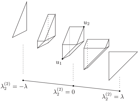
Δ[λ,λ],𝒖=(u1,u2,u3,u4)u1.\Delta\longrightarrow[-\lambda,\lambda],\quad{\boldsymbol{u}}=(u_{1},u_{2},u_{3},u_{4})\longmapsto u_{1}.
Refer to caption
Figure 2.2: The Gelfand-Cetlin polytope for Gr(2,4)\operatorname{Gr}(2,4)

The non-smooth locus of Φ\Phi is the inverse image of the edge of Δ\Delta defined by u1==u4u_{1}=\dots=u_{4}. The fiber LtL_{t} over (t,t,t,t)Δ(t,t,t,t)\in\partial\Delta is a Lagrangian submanifold consists of 2λZZλI2n2\lambda ZZ^{*}-\lambda I_{2n} with

Z=12λ(λ+tI2λtA)modU(2)Z=\frac{1}{\sqrt{2\lambda}}\begin{pmatrix}\sqrt{\lambda+t}I_{2}\\ \sqrt{\lambda-t}A\end{pmatrix}\mod\operatorname{U}(2)

for AU(2)A\in\operatorname{U}(2). We identify U(2)\operatorname{U}(2) with U(1)×SU(2)S1×S3\operatorname{U}(1)\times\operatorname{SU}(2)\cong S^{1}\times S^{3} by

U(1)×SU(2)U(2),(a0,(a1a¯2a2a¯1))(a0001)(a1a¯2a2a¯1).\operatorname{U}(1)\times\operatorname{SU}(2)\longrightarrow\operatorname{U}(2),\quad\left(a_{0},\begin{pmatrix}a_{1}&-\overline{a}_{2}\\ a_{2}&\overline{a}_{1}\end{pmatrix}\right)\longmapsto\begin{pmatrix}a_{0}&0\\ 0&1\end{pmatrix}\begin{pmatrix}a_{1}&-\overline{a}_{2}\\ a_{2}&\overline{a}_{1}\end{pmatrix}.

Then the image of LtL_{t} under the Plücker embedding ι:Gr(2,4)(24)5\iota:\operatorname{Gr}(2,4)\to\mathbb{P}(\bigwedge^{2}\mathbb{C}^{4})\cong\mathbb{P}^{5} is given by

ι(Lt)={[λ+tλt:a0a¯2:a¯1:a0a1:a2:λtλ+ta0]||a0|2=|a1|2+|a2|2=1}.\iota(L_{t})=\Biggl{\{}\biggl{[}\sqrt{\frac{\lambda+t}{\lambda-t}}:-a_{0}\overline{a}_{2}:\overline{a}_{1}:-a_{0}a_{1}:-a_{2}:\sqrt{\frac{\lambda-t}{\lambda+t}}a_{0}\biggr{]}\Biggm{|}|a_{0}|^{2}=|a_{1}|^{2}+|a_{2}|^{2}=1\Biggr{\}}.

This expression implies the following.

Proposition 2.9.

For each t(λ,λ)t\in(-\lambda,\lambda), we define an anti-holomorphic involution τt\tau_{t} on Gr(2,4)\operatorname{Gr}(2,4) defined by

τt([Z12:Z13:Z14:Z23:Z24:Z34])=[λ+tλtZ¯34:Z¯24:Z¯23:Z¯14:Z¯13:λtλ+tZ¯12]\tau_{t}([Z_{12}:Z_{13}:Z_{14}:Z_{23}:Z_{24}:Z_{34}])=\biggl{[}\frac{\lambda+t}{\lambda-t}\overline{Z}_{34}:\overline{Z}_{24}:-\overline{Z}_{23}:-\overline{Z}_{14}:\overline{Z}_{13}:\frac{\lambda-t}{\lambda+t}\overline{Z}_{12}\biggr{]} (2.7)

Then LtL_{t} is the fixed point set of τt\tau_{t}.

Remark 2.10.

The map τ0\tau_{0} for t=0t=0 is an anti-symplectic involution as well, and satisfies τ0(Lt)=Lt\tau_{0}(L_{t})=L_{-t} for each t(λ,λ)t\in(-\lambda,\lambda).

2.5 The case of Gr(2,5)\operatorname{Gr}(2,5)

We fix λ>0\lambda>0 and identify Gr(2,5)\operatorname{Gr}(2,5) with the adjoint orbit 𝒪𝝀\mathcal{O}_{{\boldsymbol{\lambda}}} of diag(λ,λ,0,0,0)1𝔲(5)\operatorname{diag}(\lambda,\lambda,0,0,0)\in\sqrt{-1}\mathfrak{u}(5). The Gelfand-Cetlin polytope Δ\Delta is defined by

λ\displaystyle u1\displaystyle (2.8)
\displaystyle\rotatebox[origin={c}]{315.0}{$\geq$} \displaystyle\rotatebox[origin={c}]{45.0}{$\geq$} \displaystyle\rotatebox[origin={c}]{315.0}{$\geq$}
u2\displaystyle u3\displaystyle 0\displaystyle
\displaystyle\rotatebox[origin={c}]{315.0}{$\geq$} \displaystyle\rotatebox[origin={c}]{45.0}{$\geq$} \displaystyle\rotatebox[origin={c}]{315.0}{$\geq$} \displaystyle\rotatebox[origin={c}]{45.0}{$\geq$}
u4\displaystyle u5\displaystyle
\displaystyle\rotatebox[origin={c}]{315.0}{$\geq$} \displaystyle\rotatebox[origin={c}]{45.0}{$\geq$}
u6\displaystyle

We first consider the fiber L1(s1,s2,t)L_{1}(s_{1},s_{2},t) over a boundary point given by

λs2>>>s1t0>==>tt==t.\begin{aligned} \hbox to16.49995pt{$\hfill{\lambda}\hfill$}&&&&\hbox to16.49995pt{$\hfill{s_{2}}\hfill$}\\ &\rotatebox[origin={c}]{315.0}{$>$}&&\rotatebox[origin={c}]{45.0}{$>$}&&\rotatebox[origin={c}]{315.0}{$>$}\\ &&\hbox to16.49995pt{$\hfill{s_{1}}\hfill$}&&&&\hbox to16.49995pt{$\hfill{t}\hfill$}&&&&\hbox to16.49995pt{$\hfill{0}\hfill$}\\ &&&\rotatebox[origin={c}]{315.0}{$>$}&&\rotatebox[origin={c}]{45.0}{$=$}&&\rotatebox[origin={c}]{315.0}{$=$}&&\rotatebox[origin={c}]{45.0}{$>$}\\ &&&&\hbox to16.49995pt{$\hfill{t}\hfill$}&&&&\hbox to16.49995pt{$\hfill{t}\hfill$}\\ &&&&&\rotatebox[origin={c}]{315.0}{$=$}&&\rotatebox[origin={c}]{45.0}{$=$}\\ &&&&&&\hbox to16.49995pt{$\hfill{t}\hfill$}\end{aligned}.
Proposition 2.11.

The fiber L1(s1,s2,t)L_{1}(s_{1},s_{2},t) is a Lagrangian submanifold diffeomorphic to U(2)×T2S3×T3\operatorname{U}(2)\times T^{2}\cong S^{3}\times T^{3}. Moreover, L1(s1,s2,t)L_{1}(s_{1},s_{2},t) is KK-homogeneous for

K={(Pe1θ1e1θ21)U(5)|PU(2),θ1,θ2}U(2)×T2.K=\left\{\left.\begin{pmatrix}P\\ &e^{\sqrt{-1}\theta_{1}}\\ &&e^{\sqrt{-1}\theta_{2}}\\ &&&1\end{pmatrix}\in\operatorname{U}(5)\right|P\in\operatorname{U}(2),\,\theta_{1},\theta_{2}\in\mathbb{R}\right\}\cong\operatorname{U}(2)\times T^{2}.
Proof.

Note that 𝒪𝝀\mathcal{O}_{{\boldsymbol{\lambda}}} consists of matrices of the form

x=λZZ=λ(ziz¯j+wiw¯j)1i,j5\displaystyle x=\lambda ZZ^{*}=\lambda(z_{i}\overline{z}_{j}+w_{i}\overline{w}_{j})_{1\leq i,j\leq 5} (2.9)

for

Z=(z1w1z2w2z3w3z4w4z5w5)V(2,5),Z=\begin{pmatrix}z_{1}&w_{1}\\ z_{2}&w_{2}\\ z_{3}&w_{3}\\ z_{4}&w_{4}\\ z_{5}&w_{5}\end{pmatrix}\in V(2,5),

i.e.,

i=15|zi|2=i=15|wi|2=1,i=15ziw¯i=0.\displaystyle\sum_{i=1}^{5}|z_{i}|^{2}=\sum_{i=1}^{5}|w_{i}|^{2}=1,\quad\sum_{i=1}^{5}z_{i}\overline{w}_{i}=0. (2.10)

Since the upper-left 2×22\times 2 submatrix of x=λ(ziz¯j+wiw¯j)L1(s1,s2,t)x=\lambda(z_{i}\overline{z}_{j}+w_{i}\overline{w}_{j})\in L_{1}(s_{1},s_{2},t) satisfies

x(2)=λ(|z1|2+|w1|2z1z¯2+w1w¯2z2z¯1+w2w¯1|z2|2+|w2|2)=(t00t),\displaystyle x^{(2)}=\lambda\begin{pmatrix}|z_{1}|^{2}+|w_{1}|^{2}&z_{1}\overline{z}_{2}+w_{1}\overline{w}_{2}\\ z_{2}\overline{z}_{1}+w_{2}\overline{w}_{1}&|z_{2}|^{2}+|w_{2}|^{2}\end{pmatrix}=\begin{pmatrix}t&0\\ 0&t\end{pmatrix}, (2.11)

we have

λt(z1w1z2w2)U(2),\displaystyle\sqrt{\frac{\lambda}{t}}\begin{pmatrix}z_{1}&w_{1}\\ z_{2}&w_{2}\end{pmatrix}\in\operatorname{U}(2), (2.12)

and in particular, |z1|2+|z2|2=|w1|2+|w2|2=t/λ|z_{1}|^{2}+|z_{2}|^{2}=|w_{1}|^{2}+|w_{2}|^{2}=t/\lambda. Then the condition (2.10) implies

|z3|2+|z4|2+|z5|2\displaystyle|z_{3}|^{2}+|z_{4}|^{2}+|z_{5}|^{2} =(λt)/λ,\displaystyle=(\lambda-t)/\lambda, (2.13)
|w3|2+|w4|2+|w5|2\displaystyle|w_{3}|^{2}+|w_{4}|^{2}+|w_{5}|^{2} =(λt)/λ,\displaystyle=(\lambda-t)/\lambda, (2.14)
z3w¯3+z4w¯4+z5w¯5\displaystyle z_{3}\overline{w}_{3}+z_{4}\overline{w}_{4}+z_{5}\overline{w}_{5} =0.\displaystyle=0. (2.15)

On the other hand, the conditions trx(3)=s1+t\operatorname{tr}x^{(3)}=s_{1}+t, trx(4)=λ+s2\operatorname{tr}x^{(4)}=\lambda+s_{2} imply

|z3|2+|w3|2\displaystyle|z_{3}|^{2}+|w_{3}|^{2} =(s1t)/λ,\displaystyle=(s_{1}-t)/\lambda, (2.16)
|z4|2+|w4|2\displaystyle|z_{4}|^{2}+|w_{4}|^{2} =(λs1+s2t)/λ,\displaystyle=(\lambda-s_{1}+s_{2}-t)/\lambda, (2.17)
|z5|2+|w5|2\displaystyle|z_{5}|^{2}+|w_{5}|^{2} =(λs2)/λ.\displaystyle=(\lambda-s_{2})/\lambda. (2.18)

After the right SU(2)\operatorname{SU}(2)-action on (z,w)(z,w), we may assume that (z5,w5)=((λs2)/λ,0)(z_{5},w_{5})=\bigl{(}\sqrt{(\lambda-s_{2})/\lambda},0\bigr{)}. Then (2.13), (2.14), and (2.15) become

|z3|2+|z4|2\displaystyle|z_{3}|^{2}+|z_{4}|^{2} =(s2t)/λ,\displaystyle=(s_{2}-t)/\lambda,
|w3|2+|w4|2\displaystyle|w_{3}|^{2}+|w_{4}|^{2} =(λt)/λ,\displaystyle=(\lambda-t)/\lambda,
z3w¯3+z4w¯4\displaystyle z_{3}\overline{w}_{3}+z_{4}\overline{w}_{4} =0,\displaystyle=0,

which mean that the 2×22\times 2 submatrix (zi,wi)i=3,4(z_{i},w_{i})_{i=3,4} has the form

(z3w3z4w4)=((s2t)/λa(λt)/λb¯c(s2t)/λb(λt)/λa¯c)\begin{pmatrix}z_{3}&w_{3}\\ z_{4}&w_{4}\end{pmatrix}=\begin{pmatrix}\sqrt{(s_{2}-t)/\lambda}\,a&-\sqrt{(\lambda-t)/\lambda}\,\overline{b}c\\ \sqrt{(s_{2}-t)/\lambda}\,b&\sqrt{(\lambda-t)/\lambda}\,\overline{a}c\end{pmatrix}

for some

(ab¯ba¯)SU(2),cU(1).\begin{pmatrix}a&-\overline{b}\\ b&\overline{a}\end{pmatrix}\in\operatorname{SU}(2),\quad c\in\operatorname{U}(1).

Combining this with (2.16) and (2.17) we have

|a|2=λs1λs2,|b|2=s1s2λs2,|a|^{2}=\frac{\lambda-s_{1}}{\lambda-s_{2}},\quad|b|^{2}=\frac{s_{1}-s_{2}}{\lambda-s_{2}},

and hence

(z3w3z4w4)=1λ(λs2)((s2t)(λs1)e1θ1(λt)(s1s2)e1θ2c(s2t)(s1s2)e1θ2(λt)(λs1)e1θ1c)\begin{pmatrix}z_{3}&w_{3}\\ z_{4}&w_{4}\end{pmatrix}=\frac{1}{\sqrt{\lambda(\lambda-s_{2})}}\begin{pmatrix}\sqrt{(s_{2}-t)(\lambda-s_{1})}\,e^{\sqrt{-1}\theta_{1}}&-\sqrt{(\lambda-t)(s_{1}-s_{2})}\,e^{-\sqrt{-1}\theta_{2}}c\\ \sqrt{(s_{2}-t)(s_{1}-s_{2})}\,e^{\sqrt{-1}\theta_{2}}&\sqrt{(\lambda-t)(\lambda-s_{1})}\,e^{-\sqrt{-1}\theta_{1}}c\end{pmatrix}

for some θ1,θ2\theta_{1},\theta_{2}\in\mathbb{R}. After the action of

{(100e1φ)U(2)|φ}U(1)\left\{\left.\begin{pmatrix}1&0\\ 0&e^{\sqrt{-1}\varphi}\end{pmatrix}\in\operatorname{U}(2)\right|\varphi\in\mathbb{R}\right\}\cong\operatorname{U}(1)

from the right, we may assume that

(z3w3z4w4)=1λ(λs2)((s2t)(λs1)e1θ1(λt)(s1s2)e1θ1(s2t)(s1s2)e1θ2(λt)(λs1)e1θ2).\begin{pmatrix}z_{3}&w_{3}\\ z_{4}&w_{4}\end{pmatrix}=\frac{1}{\sqrt{\lambda(\lambda-s_{2})}}\begin{pmatrix}\sqrt{(s_{2}-t)(\lambda-s_{1})}\,e^{\sqrt{-1}\theta_{1}}&-\sqrt{(\lambda-t)(s_{1}-s_{2})}\,e^{\sqrt{-1}\theta_{1}}\\ \sqrt{(s_{2}-t)(s_{1}-s_{2})}\,e^{\sqrt{-1}\theta_{2}}&\sqrt{(\lambda-t)(\lambda-s_{1})}\,e^{\sqrt{-1}\theta_{2}}\end{pmatrix}.

Therefore Z=(zi,wi)iZ=(z_{i},w_{i})_{i} is normalized as

(z1w1z5w5)=(z1w1z2w2(s2t)(λs1)/λ(λs2)e1θ1(λt)(s1s2)/λ(λs2)e1θ1(s2t)(s1s2)/λ(λs2)e1θ2(λt)(λs1)/λ(λs2)e1θ2(λs2)/λ0)\begin{pmatrix}z_{1}&w_{1}\\ \vdots&\vdots\\ z_{5}&w_{5}\\ \end{pmatrix}=\begin{pmatrix}z_{1}&w_{1}\\ z_{2}&w_{2}\\ \sqrt{(s_{2}-t)(\lambda-s_{1})/\lambda(\lambda-s_{2})}\,e^{\sqrt{-1}\theta_{1}}&-\sqrt{(\lambda-t)(s_{1}-s_{2})/\lambda(\lambda-s_{2})}\,e^{\sqrt{-1}\theta_{1}}\\ \sqrt{(s_{2}-t)(s_{1}-s_{2})/\lambda(\lambda-s_{2})}\,e^{\sqrt{-1}\theta_{2}}&\sqrt{(\lambda-t)(\lambda-s_{1})/\lambda(\lambda-s_{2})}\,e^{\sqrt{-1}\theta_{2}}\\ \sqrt{(\lambda-s_{2})/\lambda}&0\end{pmatrix}

with (2.12), which implies that L1(s1,s2,t)L_{1}(s_{1},s_{2},t) is a KK-orbit and diffeomorphic to U(2)×T2\operatorname{U}(2)\times T^{2}.

The assertion that L1(s1,s2,t)L_{1}(s_{1},s_{2},t) is Lagrangian follows from the KK-homogeneity as in the cases of Fl(3)\operatorname{Fl}(3) and Gr(n,2n)\operatorname{Gr}(n,2n). ∎

Next we consider the fiber L2(s1,s2,t)L_{2}(s_{1},s_{2},t) over

λt>==tt0==>>ts1>>s2.\begin{aligned} \hbox to16.49995pt{$\hfill{\lambda}\hfill$}&&&&\hbox to16.49995pt{$\hfill{t}\hfill$}\\ &\rotatebox[origin={c}]{315.0}{$>$}&&\rotatebox[origin={c}]{45.0}{$=$}&&\rotatebox[origin={c}]{315.0}{$=$}\\ &&\hbox to16.49995pt{$\hfill{t}\hfill$}&&&&\hbox to16.49995pt{$\hfill{t}\hfill$}&&&&\hbox to16.49995pt{$\hfill{0}\hfill$}\\ &&&\rotatebox[origin={c}]{315.0}{$=$}&&\rotatebox[origin={c}]{45.0}{$=$}&&\rotatebox[origin={c}]{315.0}{$>$}&&\rotatebox[origin={c}]{45.0}{$>$}\\ &&&&\hbox to16.49995pt{$\hfill{t}\hfill$}&&&&\hbox to16.49995pt{$\hfill{s_{1}}\hfill$}\\ &&&&&\rotatebox[origin={c}]{315.0}{$>$}&&\rotatebox[origin={c}]{45.0}{$>$}\\ &&&&&&\hbox to16.49995pt{$\hfill{s_{2}}\hfill$}\end{aligned}.

Suppose that x=λ(ziz¯j+wiw¯j)1i,j5L2(s1,s2,t)x=\lambda(z_{i}\overline{z}_{j}+w_{i}\overline{w}_{j})_{1\leq i,j\leq 5}\in L_{2}(s_{1},s_{2},t). The condition that x(3)=λ(ziz¯j+wiw¯j)1i,j3x^{(3)}=\lambda(z_{i}\overline{z}_{j}+w_{i}\overline{w}_{j})_{1\leq i,j\leq 3} has eigenvalues t,t,0t,t,0 is equivalent to

|z1|2+|z2|2+|z3|2\displaystyle|z_{1}|^{2}+|z_{2}|^{2}+|z_{3}|^{2} =t/λ,\displaystyle=t/\lambda, (2.19)
|w1|2+|w2|2+|w3|2\displaystyle|w_{1}|^{2}+|w_{2}|^{2}+|w_{3}|^{2} =t/λ,\displaystyle=t/\lambda, (2.20)
z1w¯1+z2w¯2+z3w¯3\displaystyle z_{1}\overline{w}_{1}+z_{2}\overline{w}_{2}+z_{3}\overline{w}_{3} =0,\displaystyle=0, (2.21)

and hence

λλt(z4w4z5w5)U(2).\sqrt{\frac{\lambda}{\lambda-t}}\begin{pmatrix}z_{4}&w_{4}\\ z_{5}&w_{5}\end{pmatrix}\in U(2).

On the other hand, the conditions x(1)=s2x^{(1)}=s_{2}, trx(2)=t+s1\operatorname{tr}x^{(2)}=t+s_{1}, and trx(3)=2t\operatorname{tr}x^{(3)}=2t imply

|z1|2+|w1|2\displaystyle|z_{1}|^{2}+|w_{1}|^{2} =s2/λ,\displaystyle=s_{2}/\lambda,
|z2|2+|w2|2\displaystyle|z_{2}|^{2}+|w_{2}|^{2} =(ts2+s1)/λ,\displaystyle=(t-s_{2}+s_{1})/\lambda,
|z3|2+|w3|2\displaystyle|z_{3}|^{2}+|w_{3}|^{2} =(ts1)/λ.\displaystyle=(t-s_{1})/\lambda.

Then we have the following.

Proposition 2.12.

The fiber L2(s1,s2,t)L_{2}(s_{1},s_{2},t) is a U(2)×T2\operatorname{U}(2)\times T^{2}-homogeneous Lagrangian submanifold diffeomorphic to U(2)×T2S3×T3\operatorname{U}(2)\times T^{2}\cong S^{3}\times T^{3}. Moreover, the fibers L1(s1,s2,t)L_{1}(s_{1},s_{2},t) and L2(s1,s2,t)L_{2}(s_{1},s_{2},t) satisfy

g(L2(s1,s2,t))=L1(λs1,λs2,λt)g(L_{2}(s_{1},s_{2},t))=L_{1}(\lambda-s_{1},\lambda-s_{2},\lambda-t)

for

g=(0110)U(5).g=\begin{pmatrix}0&&1\\ &\rotatebox[origin={c}]{45.0}{$\cdots$}&\\ 1&&0\end{pmatrix}\in\operatorname{U}(5).

In particular, L1(s1,s2,t)L_{1}(s_{1},s_{2},t) and L2(s1,s2,t)L_{2}(s_{1},s_{2},t) are displaceable.

The Hamiltonian isotopy invariance of the Floer cohomology over the Novikov field [FOOO09, Theorem G] implies the following.

Corollary 2.13.

For i=1,2i=1,2, we have

HF((Li(s1,s2,t),b),(Li(s1,s2,t),b);Λ)=0\mathop{H\!F}\nolimits((L_{i}(s_{1},s_{2},t),b),(L_{i}(s_{1},s_{2},t),b);\Lambda)=0

for any weak bounding cochain bb.

Remark 2.14.

Other boundary fibers have lower dimensions. For example, the fiber over

λ\displaystyle t\displaystyle
>\displaystyle\rotatebox[origin={c}]{315.0}{$>$} =\displaystyle\rotatebox[origin={c}]{45.0}{$=$} =\displaystyle\rotatebox[origin={c}]{315.0}{$=$}
t\displaystyle t\displaystyle 0\displaystyle
=\displaystyle\rotatebox[origin={c}]{315.0}{$=$} =\displaystyle\rotatebox[origin={c}]{45.0}{$=$} =\displaystyle\rotatebox[origin={c}]{315.0}{$=$} >\displaystyle\rotatebox[origin={c}]{45.0}{$>$}
t\displaystyle t\displaystyle
=\displaystyle\rotatebox[origin={c}]{315.0}{$=$} =\displaystyle\rotatebox[origin={c}]{45.0}{$=$}
t\displaystyle

consists of

(t/λ00t/λ00z4w4z5w5)modU(2)\begin{pmatrix}\sqrt{t/\lambda}&0\\ 0&\sqrt{t/\lambda}\\ 0&0\\ z_{4}&w_{4}\\ z_{5}&w_{5}\end{pmatrix}\mod\operatorname{U}(2)

with

(z4w4z5w5)(λt)/λU(2),\begin{pmatrix}z_{4}&w_{4}\\ z_{5}&w_{5}\end{pmatrix}\in\sqrt{(\lambda-t)/\lambda}\operatorname{U}(2),

which means that the fiber is diffeomorphic to U(2)\operatorname{U}(2).

3 Critical points of the potential function

Let Φ:F=F(n1,,nr,n)Δ\Phi:F=F(n_{1},\dots,n_{r},n)\to\Delta be the Gelfand-Cetlin system on the flag manifold, and {θi(k)}(i,k)I\{\theta^{(k)}_{i}\}_{(i,k)\in I} be the angle variables dual to the action variables {λi(k)}(i,k)I\{\lambda_{i}^{(k)}\}_{(i,k)\in I}. For each 𝒖=(uk(i))(i,k)IIntΔ{\boldsymbol{u}}=(u_{k}^{(i)})_{(i,k)\in I}\in\operatorname{Int}\Delta, we identify H1(L(𝒖);Λ0)H^{1}(L({\boldsymbol{u}});\Lambda_{0}) with Λ0N\Lambda_{0}^{N} by

b=(i,k)Ixi(k)dθi(k)H1(L(𝒖);Λ0)𝒙=(xi(k))(i,k)IΛ0N,b=\sum_{(i,k)\in I}x^{(k)}_{i}d\theta^{(k)}_{i}\in H^{1}(L({\boldsymbol{u}});\Lambda_{0})\longleftrightarrow{\boldsymbol{x}}=(x^{(k)}_{i})_{(i,k)\in I}\in\Lambda_{0}^{N},

and set

yi(k)\displaystyle y_{i}^{(k)} =exi(k)Tui(k),(i,k)I,\displaystyle=e^{x_{i}^{(k)}}T^{u_{i}^{(k)}},\qquad(i,k)\in I,
Qj\displaystyle Q_{j} =Tλnj,j=1,,r+1.\displaystyle=T^{\lambda_{n_{j}}},\qquad j=1,\dots,r+1.
Theorem 3.1 ([NNU10, Theorem 10.1]).

For any interior point 𝐮IntΔ{\boldsymbol{u}}\in\operatorname{Int}\Delta, we have an inclusion H1(L(𝐮);Λ0)^weak(L(𝐮))H^{1}(L({\boldsymbol{u}});\Lambda_{0})\subset\widehat{\mathcal{M}}_{\mathrm{weak}}(L({\boldsymbol{u}})). As a function on

𝒖IntΔH1(L(𝒖);Λ0)IntΔ×Λ0N,\bigcup_{{\boldsymbol{u}}\in\operatorname{Int}\Delta}H^{1}(L({\boldsymbol{u}});\Lambda_{0})\cong\operatorname{Int}\Delta\times\Lambda_{0}^{N},

the potential function is given by

𝔓𝔒(𝒖,𝒙)=(i,k)I(yi(k+1)yi(k)+yi(k)yi+1(k+1)),\mathfrak{PO}({\boldsymbol{u}},{\boldsymbol{x}})=\sum_{(i,k)\in I}\left(\frac{y_{i}^{(k+1)}}{y_{i}^{(k)}}+\frac{y_{i}^{(k)}}{y_{i+1}^{(k+1)}}\right),

where we put yi(k+1)=Qjy_{i}^{(k+1)}=Q_{j} if λi(k+1)=λnj\lambda_{i}^{(k+1)}=\lambda_{n_{j}} is a constant function.

Example 3.2.

We identify the 3-dimensional flag manifold Fl(3)\operatorname{Fl}(3) with the adjoint orbit of 𝝀=diag(λ1,λ2,λ3){\boldsymbol{\lambda}}=\operatorname{diag}(\lambda_{1},\lambda_{2},\lambda_{3}). The potential function is given by

𝔓𝔒\displaystyle\mathfrak{PO} =ex1Tu1+λ1+ex1Tu1λ2+ex2Tu2+λ2\displaystyle=e^{-x_{1}}T^{-u_{1}+\lambda_{1}}+e^{x_{1}}T^{u_{1}-\lambda_{2}}+e^{-x_{2}}T^{-u_{2}+\lambda_{2}}
+ex2Tu2λ3+ex1x3Tu1u3+ex2+x3Tu2+u3\displaystyle\qquad+e^{x_{2}}T^{u_{2}-\lambda_{3}}+e^{x_{1}-x_{3}}T^{u_{1}-u_{3}}+e^{-x_{2}+x_{3}}T^{-u_{2}+u_{3}}
=Q1y1+y1Q2+Q2y2+y2Q3+y1y3+y3y2.\displaystyle=\frac{Q_{1}}{y_{1}}+\frac{y_{1}}{Q_{2}}+\frac{Q_{2}}{y_{2}}+\frac{y_{2}}{Q_{3}}+\frac{y_{1}}{y_{3}}+\frac{y_{3}}{y_{2}}.

The potential function 𝔓𝔒\mathfrak{PO} has six critical points given by

y1\displaystyle y_{1} =y32/y2,\displaystyle={y_{3}^{2}}/{y_{2}},
y2\displaystyle y_{2} =±Q3(y3+Q2),\displaystyle=\pm\sqrt{Q_{3}(y_{3}+Q_{2})},
y3\displaystyle y_{3} =Q1Q2Q33,e2π1/3Q1Q2Q33,e4π1/3Q1Q2Q33.\displaystyle=\sqrt[3]{Q_{1}Q_{2}Q_{3}},\ e^{2\pi\sqrt{-1}/3}\sqrt[3]{Q_{1}Q_{2}Q_{3}},\ e^{4\pi\sqrt{-1}/3}\sqrt[3]{Q_{1}Q_{2}Q_{3}}.

It is easy to see that all critical points are non-degenerate and have the same valuation which lies in the interior of the Gelfand-Cetlin polytope. Hence we have as many critical points as dimH(Fl(3))=6\dim H^{*}(\operatorname{Fl}(3))=6 in this case. One can show, using the presentation of the quantum cohomology in [GK95, Theorem 1], that the set of eigenvalues of the quantum cup product by c1(Fl(3))c_{1}(\operatorname{Fl}(3)) coincides with the set of critical values of the potential function.

The Floer differential 𝔪1b\mathfrak{m}_{1}^{b} is trivial for each critical point (𝒖,𝒙)({\boldsymbol{u}},{\boldsymbol{x}}) of 𝔓𝔒\mathfrak{PO}, and the corresponding Floer cohomology is given by

HF((L(𝒖),b),(L(𝒖),b);Λ0)H(L(𝒖);Λ0)H(T3;Λ0).\mathop{H\!F}\nolimits((L({\boldsymbol{u}}),b),(L({\boldsymbol{u}}),b);\Lambda_{0})\cong H^{*}(L({\boldsymbol{u}});\Lambda_{0})\cong H^{*}(T^{3};\Lambda_{0}).
Example 3.3.

We identify Gr(2,4)\operatorname{Gr}(2,4) with the adjoint orbit of diag(2λ,2λ,0,0)\operatorname{diag}(2\lambda,2\lambda,0,0). Setting Q=T2λQ=T^{2\lambda}, the potential function is given by

𝔓𝔒\displaystyle\mathfrak{PO} =ex2Tu2+2λ+ex1+x2Tu1+u2+ex1x3Tu1u3\displaystyle=e^{-x_{2}}T^{-u_{2}+2\lambda}+e^{-x_{1}+x_{2}}T^{-u_{1}+u_{2}}+e^{x_{1}-x_{3}}T^{u_{1}-u_{3}}
+ex3Tu3+ex2x4Tu2u4+ex3+x4Tu3+u4\displaystyle\qquad+e^{x_{3}}T^{u_{3}}+e^{x_{2}-x_{4}}T^{u_{2}-u_{4}}+e^{-x_{3}+x_{4}}T^{-u_{3}+u_{4}}
=Qy2+y2y1+y1y3+y3+y2y4+y4y3.\displaystyle=\frac{Q}{y_{2}}+\frac{y_{2}}{y_{1}}+\frac{y_{1}}{y_{3}}+y_{3}+\frac{y_{2}}{y_{4}}+\frac{y_{4}}{y_{3}}. (3.1)

This function has four critical points

(y1,y2,y3,y4)=((1)iQ24,1iQ344,1i4Q4,(1)iQ24)(y_{1},y_{2},y_{3},y_{4})=\left((-1)^{i}\sqrt[4]{Q^{2}},\sqrt{-1}^{i}\sqrt[4]{\frac{Q^{3}}{4}},\sqrt{-1}^{i}\sqrt[4]{4Q},(-1)^{i}\sqrt[4]{Q^{2}}\right)

for i=0,1,2,3i=0,1,2,3, and the corresponding critical values are

𝔓𝔒=421iQ4.\displaystyle\mathfrak{PO}=4\sqrt{2}\sqrt{-1}^{i}\sqrt[4]{Q}. (3.2)

Since dimH(Gr(2,4))=6\dim H^{*}(\operatorname{Gr}(2,4))=6, one has less critical point than dimH(Gr(2,4))\dim H^{*}(\operatorname{Gr}(2,4)). These critical points are non-degenerate and have a common valuation

𝒖0=(λ,3λ/2,λ/2,λ)IntΔ.{\boldsymbol{u}}_{0}=(\lambda,3\lambda/2,\lambda/2,\lambda)\in\operatorname{Int}\Delta.

Hence there exist four weak bounding cochains b0,,b3b_{0},\dots,b_{3} such that

HF((L(𝒖0),bi),(L(𝒖0),bi);Λ0)H(L(𝒖0);Λ0)H(T4;Λ0)\mathop{H\!F}\nolimits((L({\boldsymbol{u}}_{0}),b_{i}),(L({\boldsymbol{u}}_{0}),b_{i});\Lambda_{0})\cong H^{*}(L({\boldsymbol{u}}_{0});\Lambda_{0})\cong H^{*}(T^{4};\Lambda_{0})

for i=0,1,2,3i=0,1,2,3. One can show, using the presentation of the quantum cohomology in [ST97, Theorem 0.1], that the set eigenvalues of the quantum cup product by c1(Gr(2,4))c_{1}(\operatorname{Gr}(2,4)) consists of the four critical values of the potential function and the zero eigenvalue with multiplicity two.

Example 3.4.

We identify Gr(2,5)\operatorname{Gr}(2,5) with the adjoint orbit of diag(λ,λ,0,0,0)\operatorname{diag}(\lambda,\lambda,0,0,0). Since the Gelfand-Cetlin polytope is defined by (2.8), the potential function is given by

𝔓𝔒=Qy2+y2y1+y1y3+y2y4+y4y3+y3y5+y5+y4y6+y6y5.\displaystyle\mathfrak{PO}=\frac{Q}{y_{2}}+\frac{y_{2}}{y_{1}}+\frac{y_{1}}{y_{3}}+\frac{y_{2}}{y_{4}}+\frac{y_{4}}{y_{3}}+\frac{y_{3}}{y_{5}}+y_{5}+\frac{y_{4}}{y_{6}}+\frac{y_{6}}{y_{5}}. (3.3)

This function has ten critical points defined by

y65=Q5,Qy4=y6(y63y42),y_{6}^{5}=Q^{5},\quad Qy_{4}=y_{6}(y_{6}^{3}-y_{4}^{2}),

and

y1=Qy6,y2=Qy5,y3=Qy4,y5=y62y4.y_{1}=\frac{Q}{y_{6}},\quad y_{2}=\frac{Q}{y_{5}},\quad y_{3}=\frac{Q}{y_{4}},\quad y_{5}=\frac{y_{6}^{2}}{y_{4}}.

The set

{5(ζ5i+ζ5j)Q1/5|ζ5=exp(2π1/5) and 0i<j4}\displaystyle\left\{5(\zeta_{5}^{i}+\zeta_{5}^{j})Q^{1/5}\mathrel{}\middle|\mathrel{}\zeta_{5}=\exp(2\pi\sqrt{-1}/5)\text{ and }0\leq i<j\leq 4\right\} (3.4)

of critical values of the potential function coincides with the set of eigenvalues of the quantum cup product by c1(Gr(2,5))c_{1}(\operatorname{Gr}(2,5)).

4 Floer cohomologies of non-torus fibers

We briefly recall the construction of the AA_{\infty} structure {𝔪k}k0\{\mathfrak{m}_{k}\}_{k\geq 0}, omitting various technical details. Let LL be a spin, oriented, and compact Lagrangian submanifold in a symplectic manifold (X,ω)(X,\omega). For an almost complex structure JJ compatible with ω\omega, let k+1(J,β)\mathcal{M}_{k+1}(J,\beta) be the moduli space of stable JJ-holomorphic maps v:(Σ,Σ)(X,L)v:(\Sigma,\partial\Sigma)\to(X,L) from a bordered Riemann surface Σ\Sigma in the class βπ2(X,L)\beta\in\pi_{2}(X,L) of genus zero with (k+1)(k+1) boundary marked points z0,z1,,zkΣz_{0},z_{1},\dots,z_{k}\in\partial\Sigma. Then 𝔪k=βπ2(X,L)Tβω𝔪k,β:H(L;Λ0)kH(L;Λ0)\mathfrak{m}_{k}=\sum_{\beta\in\pi_{2}(X,L)}T^{\beta\cap\omega}\mathfrak{m}_{k,\beta}\colon H^{*}(L;\Lambda_{0})^{\otimes k}\to H^{*}(L;\Lambda_{0}) is defined by

𝔪k,β(x1,,xk)=(ev0)(ev1x1evkxk),\mathfrak{m}_{k,\beta}(x_{1},\dots,x_{k})=(\operatorname{ev}_{0})_{*}(\operatorname{ev}_{1}^{*}x_{1}\cup\dots\cup\operatorname{ev}_{k}^{*}x_{k}),

where evi:k+1(J,β)L\operatorname{ev}_{i}\colon\mathcal{M}_{k+1}(J,\beta)\to L, [v,(z0,,zk)]v(zi)[v,(z_{0},\dots,z_{k})]\mapsto v(z_{i}) is the evaluation map at the iith marked point.

4.1 Holomorphic disks in (Fl(3),L0)(\operatorname{Fl}(3),L_{0})

We identify Fl(3)\operatorname{Fl}(3) with the adjoint orbit of diag(λ1,0,λ2)\operatorname{diag}(\lambda_{1},0,-\lambda_{2}) for λ1,λ2>0\lambda_{1},\lambda_{2}>0 as in Subsection 2.3. Note that the symplectic form and the first Chern class are given by ω=λ1ω1+λ2ω2\omega=\lambda_{1}\omega_{\mathbb{P}_{1}}+\lambda_{2}\omega_{\mathbb{P}_{2}} and c1(Fl(3))=2(ω1+ω2)c_{1}(\operatorname{Fl}(3))=2(\omega_{\mathbb{P}_{1}}+\omega_{\mathbb{P}_{2}}), respectively.

Recall that the homotopy group π2(Fl(3))2\pi_{2}(\operatorname{Fl}(3))\cong\mathbb{Z}^{2} is generated by 1-dimensional Schubert varieties X1X_{1} and X2X_{2}, which are rational curves of bidegree (1,0)(1,0) and (0,1)(0,1) in 1×22×2\mathbb{P}_{1}\times\mathbb{P}_{2}\cong\mathbb{P}^{2}\times\mathbb{P}^{2}, respectively. Since L0L_{0} is diffeomorphic to SU(2)S3\operatorname{SU}(2)\cong S^{3}, we have π1(L0)=π2(L0)=0\pi_{1}(L_{0})=\pi_{2}(L_{0})=0. The long exact sequence of homotopy groups yields

π2(Fl(3),L0)π2(Fl(3))2.\pi_{2}(\operatorname{Fl}(3),L_{0})\cong\pi_{2}(\operatorname{Fl}(3))\cong\mathbb{Z}^{2}.

Let β1\beta_{1}, β2\beta_{2} be generators of π2(Fl(3),L0)\pi_{2}(\operatorname{Fl}(3),L_{0}) corresponding to X1X_{1} and X2X_{2}, respectively. The symplectic area of βi\beta_{i} is given by

βiω=[Xi](λ1ω1+λ2ω2)=λi.\beta_{i}\cap\omega=[X_{i}]\cap(\lambda_{1}\omega_{\mathbb{P}_{1}}+\lambda_{2}\omega_{\mathbb{P}_{2}})=\lambda_{i}.

Let τ\tau be the anti-holomorphic involution on Fl(3)\operatorname{Fl}(3) defined in (2.5). For a holomorphic disk v:(D2,D2)(Fl(3),L0)v:(D^{2},\partial D^{2})\to(\operatorname{Fl}(3),L_{0}), we define a new holomorphic disk τv:(D2,D2)(Fl(3),L0)\tau_{*}v:(D^{2},\partial D^{2})\to(\operatorname{Fl}(3),L_{0}) by

τv(z)=τ(v(z¯)).\tau_{*}v(z)=\tau(v(\overline{z})).

Since L0L_{0} is the fixed point set of τ\tau, one can glue vv and τv\tau_{*}v along the boundary to obtain a holomorphic curve w=v#τv:1Fl(3)w=v\#\tau_{*}v:\mathbb{P}^{1}\to\operatorname{Fl}(3). The induced involution on π2(Fl(3),L0)\pi_{2}(\operatorname{Fl}(3),L_{0}), which is also denoted by τ\tau_{*}, is given by τβ1=β2\tau_{*}\beta_{1}=\beta_{2}. If vv represents β1\beta_{1} or β2\beta_{2}, then [w]=β1+β2=[X1]+[X2][w]=\beta_{1}+\beta_{2}=[X_{1}]+[X_{2}], i.e., ww is a rational curve of bidegree (1,1)(1,1).

Let μL0:π2(Fl(3),L0)\mu_{L_{0}}:\pi_{2}(\operatorname{Fl}(3),L_{0})\to\mathbb{Z} be the Maslov index. If we assume λ1=λ2\lambda_{1}=\lambda_{2} so that τ\tau is an anti-symplectic involution, then we have

μL0(βi)=12(μL0(βi)+μL0(τβi))=([X1]+[X2])c1(Fl(3))=4\mu_{L_{0}}(\beta_{i})=\frac{1}{2}(\mu_{L_{0}}(\beta_{i})+\mu_{L_{0}}(\tau_{*}\beta_{i}))=([X_{1}]+[X_{2}])\cap c_{1}(\operatorname{Fl}(3))=4

for i=1,2i=1,2. Since the symplectic form ω\omega and the Lagrangian submanifold L0L_{0} depend continuously on λ1,λ2>0\lambda_{1},\lambda_{2}>0, the Maslov index μL0(β1)=μL0(β2)=4\mu_{L_{0}}(\beta_{1})=\mu_{L_{0}}(\beta_{2})=4 is independent of λ1,λ2\lambda_{1},\lambda_{2}.

To describe holomorphic disks with Lagrangian boundary condition, we identify the unit disk D2D^{2} with the upper half plane =+\mathbb{H}=\mathbb{H}_{+}.

Proposition 4.1.

Let w:1Fl(3)w\colon\mathbb{P}^{1}\to\operatorname{Fl}(3) be a holomorphic curve of bidegree (1,1)(1,1) such that w({})L0w(\mathbb{R}\cup\{\infty\})\subset L_{0}. After the SU(2)\operatorname{SU}(2)-action, we may assume

w()=([1:0:λ1/λ2],[1:0:λ2/λ1]).w(\infty)=([1:0:\sqrt{\lambda_{1}/\lambda_{2}}],[1:0:-\sqrt{\lambda_{2}/\lambda_{1}}]). (4.1)

We can write

w(0)=([a1:a2:λ1/λ2],[a¯1:a¯2:λ2/λ1])L0w(0)=\Bigl{(}\bigl{[}a_{1}:a_{2}:\sqrt{\lambda_{1}/\lambda_{2}}\bigr{]},\bigl{[}\overline{a}_{1}:\overline{a}_{2}:-\sqrt{\lambda_{2}/\lambda_{1}}\bigr{]}\Bigr{)}\in L_{0} (4.2)

for some (a1,a2)S3{(1,0)}(a_{1},a_{2})\in S^{3}\setminus\{(1,0)\}. Then ww is given by

w(z)=([cz+a1:a2:λ1/λ2(cz+1)],[c¯z+a¯1:a¯2:λ2/λ1(c¯z+1)])w(z)=\Bigl{(}\bigl{[}cz+a_{1}:a_{2}:\sqrt{\lambda_{1}/\lambda_{2}}(cz+1)\bigr{]},\bigl{[}\overline{c}z+\overline{a}_{1}:\overline{a}_{2}:-\sqrt{\lambda_{2}/\lambda_{1}}(\overline{c}z+1)\bigr{]}\Bigr{)}

with c/c¯=(a11)/(a¯11)c/\overline{c}=-(a_{1}-1)/(\overline{a}_{1}-1).

Remark 4.2.

After the action of

{gPSL(2,)|g(0)=0,g()=}>0\{g\in\operatorname{PSL}(2,\mathbb{R})\,|\,g(0)=0,\,g(\infty)=\infty\}\cong\mathbb{R}_{>0}

on \mathbb{H}, we may assume that |c|=1|c|=1.

Proof.

The assumptions (4.1) and (4.2) implies that ww has the form

w(z)=([c1z+a1:a2:λ1/λ2(c1z+1)],[c2z+a¯1:a¯2:λ2/λ1(c2z+1)])w(z)=\Bigl{(}\bigl{[}c_{1}z+a_{1}:a_{2}:\sqrt{\lambda_{1}/\lambda_{2}}(c_{1}z+1)\bigr{]},\bigl{[}c_{2}z+\overline{a}_{1}:\overline{a}_{2}:-\sqrt{\lambda_{2}/\lambda_{1}}(c_{2}z+1)\bigr{]}\Bigr{)}

for some c1,c2c_{1},c_{2}\in\mathbb{C}^{*}. The Plücker relation

0\displaystyle 0 =(c1z+a1)(c2z+a¯1)|a2|2+(c1z+1)(c2z+1)\displaystyle=-(c_{1}z+a_{1})(c_{2}z+\overline{a}_{1})-|a_{2}|^{2}+(c_{1}z+1)(c_{2}z+1)
=(c1a1c1+c2a¯1c2)z\displaystyle=(c_{1}-a_{1}c_{1}+c_{2}-\overline{a}_{1}c_{2})z

implies c1(a¯11)+c2(a1)=0c_{1}(\overline{a}_{1}-1)+c_{2}(a-1)=0. On the other hand, the Lagrangian boundary condition w()L0w(\mathbb{R})\subset L_{0} implies that

c1x+a1c1x+1=c2¯x+a1c2¯x+1,a2c1x+1=a2c2¯x+1,x,\frac{c_{1}x+a_{1}}{c_{1}x+1}=\frac{\overline{c_{2}}x+a_{1}}{\overline{c_{2}}x+1},\quad\frac{a_{2}}{c_{1}x+1}=\frac{a_{2}}{\overline{c_{2}}x+1},\quad x\in\mathbb{R},

which means c2=c1¯c_{2}=\overline{c_{1}}. ∎

Note that argc\arg c is determined by a1a_{1} up to sign, and the sign corresponds to whether v=w|v=w|_{\mathbb{H}} represents β1\beta_{1} or β2\beta_{2}. Namely any holomorphic disk in the class βi\beta_{i} satisfying (4.1) and (4.2) is uniquely determined by (a1,a2)(a_{1},a_{2}) for i=1,2i=1,2.

Example 4.3.

Suppose that (a1,a2)=(1,0)(a_{1},a_{2})=(-1,0). Then c=±1c=\pm\sqrt{-1}, and the corresponding holomorphic disks are given by

v±(z)=([z±1:0:λ1λ2(z1)],[z1:0:λ2λ1(z±1)]).v_{\pm}(z)=\Bigl{(}\bigl{[}z\pm\sqrt{-1}:0:\sqrt{\frac{\lambda_{1}}{\lambda_{2}}}(z\mp\sqrt{-1})\bigr{]},\bigl{[}z\mp\sqrt{-1}:0:-\sqrt{\frac{\lambda_{2}}{\lambda_{1}}}(z\pm\sqrt{-1})\bigr{]}\Bigr{)}.

It is easy to see that the image v+()v_{+}(\mathbb{H}) (resp. v()v_{-}(\mathbb{H})) is the inverse image of the edge of Δ\Delta given by u1(1)=u1(2)u^{(1)}_{1}=u^{(2)}_{1} and u2(2)=0u^{(2)}_{2}=0 (resp. u1(1)=u2(2)u^{(1)}_{1}=u^{(2)}_{2} and u1(2)=0u^{(2)}_{1}=0), which is the upper (resp. lower) vertical edge emanating from the vertex 𝟎=(0,0,0){\boldsymbol{0}}=(0,0,0). The generators β1,β2\beta_{1},\beta_{2} of π2(Fl(3),L0)\pi_{2}(\operatorname{Fl}(3),L_{0}) are represented by v+v_{+} and vv_{-} respectively.

4.2 Floer cohomology of the SU(2)\operatorname{SU}(2)-fiber in Fl(3)\operatorname{Fl}(3)

Let JJ be the standard complex structure on Fl(3)\operatorname{Fl}(3). Since the fiber L0L_{0} is SU(2)\operatorname{SU}(2)-homogeneous, [EL, Proposition 3.2.1] implies the following.

Proposition 4.4.

Any JJ-holomorphic disk in (Fl(3),L0)(\operatorname{Fl}(3),L_{0}) is Fredholm regular. Hence the moduli space k+1reg(J,β)\mathcal{M}_{k+1}^{\mathrm{reg}}(J,\beta) of JJ-holomorphic disks in the class β\beta with k+1k+1 boundary marked points is a smooth manifold of dimension

dimk+1reg(J,β)\displaystyle\dim\mathcal{M}_{k+1}^{\mathrm{reg}}(J,\beta) =dimL0+μL0(β)+k+13\displaystyle=\dim L_{0}+\mu_{L_{0}}(\beta)+k+1-3
=μL0(β)+k+1.\displaystyle=\mu_{L_{0}}(\beta)+k+1.

In particular, we have dim2(J,βi)=6\dim\mathcal{M}_{2}(J,\beta_{i})=6 for i=1,2i=1,2. Proposition 4.1 implies the following:

Corollary 4.5.

Let U=SU(2){1}{(a1,a2)S3|a11}U=\operatorname{SU}(2)\setminus\{1\}\cong\{(a_{1},a_{2})\in S^{3}\,|\,a_{1}\neq 1\}. Then 2(J,βi)\mathcal{M}_{2}(J,\beta_{i}) has an open dense subset diffeomorphic to SU(2)×U\operatorname{SU}(2)\times U on which the evaluation map is given by

SU(2)×UL0×L0SU(2)×SU(2),(g1,g2)(g1,g1g2).\operatorname{SU}(2)\times U\longrightarrow L_{0}\times L_{0}\cong\operatorname{SU}(2)\times\operatorname{SU}(2),\quad(g_{1},g_{2})\longmapsto(g_{1},g_{1}g_{2}).

In particular, ev:2(J,βi)L0×L0\operatorname{ev}:\mathcal{M}_{2}(J,\beta_{i})\to L_{0}\times L_{0} is generically one-to-one.

Since the minimal Maslov number is μL0(β1)=μL0(β2)=4\mu_{L_{0}}(\beta_{1})=\mu_{L_{0}}(\beta_{2})=4 and

deg𝔪1,β(x)=degx+1μL0(β),xH(L0;Λ0),\deg\mathfrak{m}_{1,\beta}(x)=\deg x+1-\mu_{L_{0}}(\beta),\quad x\in H^{*}(L_{0};\Lambda_{0}),

the only nontrivial parts of the Floer differential are

𝔪1,βi:H3(L0)H0(L0)H0(L0)H3(L0)\mathfrak{m}_{1,\beta_{i}}:H^{3}(L_{0})\cong H_{0}(L_{0})\longrightarrow H^{0}(L_{0})\cong H_{3}(L_{0})

for i=1,2i=1,2. Corollary 4.5 implies that for the class [p]H0(L0)[p]\in H_{0}(L_{0}) of a point, we have

𝔪1,βi([p])=ev0[2(J,βi)×ev1{p}]=±[L0].\mathfrak{m}_{1,\beta_{i}}([p])={\operatorname{ev}_{0}}_{*}[\mathcal{M}_{2}(J,\beta_{i}){}_{\operatorname{ev}_{1}}\!\times\{p\}]=\pm[L_{0}].

To see the sign, we use a result on the orientation of the moduli spaces of pseudo-holomorphic disks by Fukaya, Oh, Ohta, and Ono [FOOO, Theorem 1.5]. The following statement is a slightly weaker version of the result, which is sufficient for our purpose.

Theorem 4.6.

Let (X,ω)(X,\omega) be a compact symplectic manifold, and τ\tau an anti-symplectic involution on XX whose fixed point set L=Fix(τ)L=\operatorname{Fix}(\tau) is non-empty, compact, connected, and spin. Then 𝔪k,β\mathfrak{m}_{k,\beta} and 𝔪k,τβ\mathfrak{m}_{k,\tau_{*}\beta} satisfy

𝔪k,β(P1,,Pk)=(1)ϵ𝔪k,τβ(Pk,,P1),\mathfrak{m}_{k,\beta}(P_{1},\dots,P_{k})=(-1)^{\epsilon}\mathfrak{m}_{k,\tau_{*}\beta}(P_{k},\dots,P_{1}),

where

ϵ=μL(β)2+k+1+1i<jk(degPi1)(degPj1).\epsilon=\frac{\mu_{L}(\beta)}{2}+k+1+\sum_{1\leq i<j\leq k}(\deg P_{i}-1)(\deg P_{j}-1).
Corollary 4.7.

We have 𝔪1,β1=𝔪1,β2\mathfrak{m}_{1,\beta_{1}}=\mathfrak{m}_{1,\beta_{2}} for general λ1,λ2>0\lambda_{1},\lambda_{2}>0.

Proof.

If λ1=λ2\lambda_{1}=\lambda_{2}, then τ\tau is anti-symplectic, and thus Theorem 4.6 implies

𝔪1,β1=(1)μL0(β1)/2+2𝔪1,τβ1=𝔪1,β2.\mathfrak{m}_{1,\beta_{1}}=(-1)^{\mu_{L_{0}}(\beta_{1})/2+2}\mathfrak{m}_{1,\tau_{*}\beta_{1}}=\mathfrak{m}_{1,\beta_{2}}. (4.3)

Corollary 4.5 implies that 2(J,βi)\mathcal{M}_{2}(J,\beta_{i}) depends continuously on λ1,λ2\lambda_{1},\lambda_{2}, and hence its orientation is independent of λ1,λ2\lambda_{1},\lambda_{2}. Thus (4.3) holds for general λ1,λ2\lambda_{1},\lambda_{2}. ∎

Then we have

𝔪1([p])=i=12𝔪1,βi([p])Tβiω=±(Tλ1+Tλ2)[L0],\mathfrak{m}_{1}([p])=\sum_{i=1}^{2}\mathfrak{m}_{1,\beta_{i}}([p])T^{\beta_{i}\cap\omega}=\pm(T^{\lambda_{1}}+T^{\lambda_{2}})[L_{0}],

which implies the following.

Theorem 4.8.

The Floer cohomology of L0L_{0} over the Novikov ring Λ0\Lambda_{0} is

HF(L0,L0;Λ0)Λ0/Tmin{λ1,λ2}Λ0.\mathop{H\!F}\nolimits(L_{0},L_{0};\Lambda_{0})\cong\Lambda_{0}/T^{\min\{\lambda_{1},\lambda_{2}\}}\Lambda_{0}.

Theorem 1.1 is an immediate consequence of Theorem 4.8.

4.3 Holomorphic disks in (Gr(2,4),Lt)(\operatorname{Gr}(2,4),L_{t})

We identify Gr(2,4)\operatorname{Gr}(2,4) with the adjoint orbit of diag(λ,λ,λ,λ)\operatorname{diag}(\lambda,\lambda,-\lambda,-\lambda) for λ>0\lambda>0. Note that the Kostant-Kirillov form and the first Chern class are given by

ω=2λωFS,c1(Gr(2,4))=4ωFS,\omega=2\lambda\omega_{\mathrm{FS}},\quad c_{1}(\operatorname{Gr}(2,4))=4\omega_{\mathrm{FS}},

respectively, where ωFS\omega_{\mathrm{FS}} is the Fubini-Study form on (24)\mathbb{P}(\bigwedge^{2}\mathbb{C}^{4}).

Recall that π2(Gr(2,4))\pi_{2}(\operatorname{Gr}(2,4))\cong\mathbb{Z} is generated by a 1-dimensional Schubert variety X1X_{1}, which is a rational curve of degree one in (24)\mathbb{P}(\bigwedge^{2}\mathbb{C}^{4}). Since π1(Gr(2,4))=π2(Lt)=0\pi_{1}(\operatorname{Gr}(2,4))=\pi_{2}(L_{t})=0 and π1(Lt)\pi_{1}(L_{t})\cong\mathbb{Z}, the exact sequence

0π2(Gr(2,4))π2(Gr(2,4),Lt)π1(Lt)00\longrightarrow\pi_{2}(\operatorname{Gr}(2,4))\longrightarrow\pi_{2}(\operatorname{Gr}(2,4),L_{t})\longrightarrow\pi_{1}(L_{t})\longrightarrow 0

implies that π2(Gr(2,4),Lt)2\pi_{2}(\operatorname{Gr}(2,4),L_{t})\cong\mathbb{Z}^{2}. Let β1,β2\beta_{1},\beta_{2} be generators of π2(Gr(2,4),Lt)\pi_{2}(\operatorname{Gr}(2,4),L_{t}) such that β1+β2=[X1]π2(Gr(2,4))\beta_{1}+\beta_{2}=[X_{1}]\in\pi_{2}(\operatorname{Gr}(2,4)).

Example 4.9.

Consider a holomorphic curve w:1Gr(2,4)w:\mathbb{P}^{1}\to\operatorname{Gr}(2,4) of degree one defined by

w(z)=[λ+tλt(z1):0:z1:z1:0:λtλ+t(z+1)].w(z)=\left[\sqrt{\frac{\lambda+t}{\lambda-t}}(z-\sqrt{-1}):0:z-\sqrt{-1}:-z-\sqrt{-1}:0:\sqrt{\frac{\lambda-t}{\lambda+t}}(z+\sqrt{-1})\right]. (4.4)

Since ww maps {}\mathbb{R}\cup\{\infty\} to LtL_{t}, the restrictions

v+\displaystyle v_{+} =w|+:(+,+)(Gr(2,4),Lt),\displaystyle=w|_{\mathbb{H}_{+}}:(\mathbb{H}_{+},\partial\mathbb{H}_{+})\longrightarrow(\operatorname{Gr}(2,4),L_{t}),
v\displaystyle v_{-} =w|:(,)(Gr(2,4),Lt)\displaystyle=w|_{\mathbb{H}_{-}}:(\mathbb{H}_{-},\partial\mathbb{H}_{-})\longrightarrow(\operatorname{Gr}(2,4),L_{t})

to the upper and lower half planes give holomorphic disks representing β1\beta_{1} and β2\beta_{2}. We define β1=[v+]\beta_{1}=[v_{+}] and β2=[v]\beta_{2}=[v_{-}]. It is easy to see that the symplectic areas of v±v_{\pm} are given by

ω(β1)=+v+ω=λ+t,ω(β2)=vω=λt.\omega(\beta_{1})=\int_{\mathbb{H}_{+}}v_{+}^{*}\omega=\lambda+t,\quad\omega(\beta_{2})=\int_{\mathbb{H}_{-}}v_{-}^{*}\omega=\lambda-t.

In the case where t=0t=0, the disk v+v_{+} sends 1\sqrt{-1}\in\mathbb{H} to v+(1)=[0:0:0:1:0:1]v_{+}(\sqrt{-1})=[0:0:0:-1:0:1], which is in the fiber Φ1(𝒖1)\Phi^{-1}({\boldsymbol{u}}_{1}) over the point 𝒖1Δ{\boldsymbol{u}}_{1}\in\Delta defined by u1(2)=u1(1)=λu_{1}^{(2)}=u_{1}^{(1)}=\lambda and u2(2)=0u_{2}^{(2)}=0 (see Figure 2.2). On the other hand, v(1)=[1:0:1:0:0:0]v_{-}(-\sqrt{-1})=[1:0:1:0:0:0] lies on the fiber over the point 𝒖2Δ{\boldsymbol{u}}_{2}\in\Delta defined by u2(2)=u1(1)=λu_{2}^{(2)}=u_{1}^{(1)}=-\lambda and u1(2)=0u_{1}^{(2)}=0.

Let τt\tau_{t} be the anti-holomorphic involution on Gr(2,4)\operatorname{Gr}(2,4) defined in (2.7). Note that (τt)(\tau_{t})_{*} is given by (τt)v(z)=τt(v(z¯))(\tau_{t})_{*}v(z)=\tau_{t}(v(-\overline{z})) for v:(,)(Gr(2,4),Lt)v:(\mathbb{H},\partial\mathbb{H})\to(\operatorname{Gr}(2,4),L_{t}). Since (τt)v+=v(\tau_{t})_{*}v_{+}=v_{-}, the induced involution on π2(Gr(2,4),Lt)\pi_{2}(\operatorname{Gr}(2,4),L_{t}) is given by (τt)β1=β2(\tau_{t})_{*}\beta_{1}=\beta_{2}. Then the Maslov index of βi\beta_{i} is given by

μLt(βi)=12(μLt(βi)+μLt((τt)βi))=[X1]c1(Gr(2,4))=4\mu_{L_{t}}(\beta_{i})=\frac{1}{2}\left(\mu_{L_{t}}(\beta_{i})+\mu_{L_{t}}((\tau_{t})_{*}\beta_{i})\right)=[X_{1}]\cap c_{1}(\operatorname{Gr}(2,4))=4

for i=1,2i=1,2.

We describe holomorphic curves w:1Gr(n,2n)w\colon\mathbb{P}^{1}\to\operatorname{Gr}(n,2n) of degree one such that w({})w(\mathbb{R}\cup\{\infty\}) is contained in the Lagrangian fiber LtL_{t}. Proposition 4.10 below is taken from [Sot01, Theorem 2.1], which is well-known in control theory (cf. e.g. [Ros70]).

Proposition 4.10.

Suppose that a holomorphic curve w:1Gr(k,n)=V~(k,n)/GL(k,)w\colon\mathbb{P}^{1}\to\operatorname{Gr}(k,n)={\widetilde{V}}(k,n)/\operatorname{GL}(k,\mathbb{C}) of degree dd is given by

w:z(IkF(z))modGL(k,)w\colon z\longmapsto\begin{pmatrix}I_{k}\\ F(z)\end{pmatrix}\mod\operatorname{GL}(k,\mathbb{C})

for a rational function F(z)F(z) with values in (nk)×K(n-k)\times K matrices. Then there exist matrix valued polynomials P(z)P(z), Q(z)Q(z) of size k×kk\times k and (nk)×k(n-k)\times k respectively such that

  1. 1.

    F(z)=Q(z)P(z)1F(z)=Q(z)P(z)^{-1}, i.e., the curve ww is given by

    w:z(P(z)Q(z))modGL(k,),w\colon z\longmapsto\begin{pmatrix}P(z)\\ Q(z)\end{pmatrix}\mod\operatorname{GL}(k,\mathbb{C}),
  2. 2.

    P(z)P(z) and Q(z)Q(z) are coprime in the sense there exist matrix valued polynomials X(z)X(z), Y(z)Y(z) such that X(z)P(z)+Y(z)Q(z)=IkX(z)P(z)+Y(z)Q(z)=I_{k}, and

  3. 3.

    deg(detP(z))=d\deg(\operatorname{det}P(z))=d.

Such P(z)P(z) and Q(z)Q(z) are unique up to multiplication of elements in GL(k,[z])\operatorname{GL}(k,\mathbb{C}[z]).

Note that (2.6) implies that the U(n)\operatorname{U}(n)-fiber LtGr(n,2n)=V~(n,2n)/GL(n,)L_{t}\subset\operatorname{Gr}(n,2n)={\widetilde{V}}(n,2n)/\operatorname{GL}(n,\mathbb{C}) consists of

(In(λt)/(λ+t)A)modGL(n,)\begin{pmatrix}I_{n}\\ \sqrt{(\lambda-t)/(\lambda+t)}\,A\end{pmatrix}\mod\operatorname{GL}(n,\mathbb{C})

for AU(n)A\in\operatorname{U}(n).

Proposition 4.11.

Let w:1Gr(n,2n)w\colon\mathbb{P}^{1}\to\operatorname{Gr}(n,2n) be a holomorphic curve of degree one such that w({})Ltw(\mathbb{R}\cup\{\infty\})\subset L_{t}, and let F(z)F(z) denote the corresponding rational function with values in n×nn\times n matrices. By the U(n)\operatorname{U}(n)-action, we assume that

F()=λtλ+tInλtλ+tU(n),F(\infty)=\sqrt{\frac{\lambda-t}{\lambda+t}}I_{n}\in\sqrt{\frac{\lambda-t}{\lambda+t}}\operatorname{U}(n), (4.5)

and set

F(0)=λtλ+tAF(0)=\sqrt{\frac{\lambda-t}{\lambda+t}}A (4.6)

for AU(n)A\in\operatorname{U}(n). Then there exist

a=(a1an)S2n1/S1=n1a=\begin{pmatrix}a_{1}\\ \vdots\\ a_{n}\end{pmatrix}\in S^{2n-1}/S^{1}=\mathbb{P}^{n-1}

and cc\in\mathbb{C}\setminus\mathbb{R} such that

A=In+(c2|c|21)aa,A=I_{n}+\left(\frac{c^{2}}{|c|^{2}}-1\right)aa^{*},

and

F(z)=λtλ+t1zc¯(zInc¯A)=λtλ+t(Incc¯zc¯aa).F(z)=\sqrt{\frac{\lambda-t}{\lambda+t}}\frac{1}{z-\overline{c}}(zI_{n}-\overline{c}A)=\sqrt{\frac{\lambda-t}{\lambda+t}}\left(I_{n}-\frac{c-\overline{c}}{z-\overline{c}}aa^{*}\right). (4.7)
Proof.

Let F(z)=Q(z)P(z)1F(z)=Q(z)P(z)^{-1} be the factorization given in Proposition 4.10. Then the assumptions (4.5), (4.6), and deg(detP(z))=1\deg(\operatorname{det}P(z))=1 imply that F(z)F(z) has the form

F(z)=λtλ+t1zc¯(zInc¯A)F(z)=\sqrt{\frac{\lambda-t}{\lambda+t}}\frac{1}{z-\overline{c}}(zI_{n}-\overline{c}A)

for some cc\in\mathbb{C}. The Lagrangian boundary condition w({})Ltw(\mathbb{R}\cup\{\infty\})\subset L_{t} implies that

1xc¯(xInc¯A)U(n)\frac{1}{x-\overline{c}}(xI_{n}-\overline{c}A)\in\operatorname{U}(n)

for any xx\in\mathbb{R}, which means c¯A+cA=(c+c¯)In\overline{c}A+cA^{*}=(c+\overline{c})I_{n}, or equivalently, c¯ARe(c)In\overline{c}A-\operatorname{Re}(c)I_{n} is skew-hermitian. Hence c¯ARe(c)In\overline{c}A-\operatorname{Re}(c)I_{n} has pure imaginary eigenvalues 1α1,,1αn\sqrt{-1}\alpha_{1},\dots,\sqrt{-1}\alpha_{n}, and can be diagonalized by some gU(n)g\in\operatorname{U}(n);

g(c¯ARe(c)In)g=diag(1α1,,1αn).g^{*}(\overline{c}A-\operatorname{Re}(c)I_{n})g=\operatorname{diag}(\sqrt{-1}\alpha_{1},\dots,\sqrt{-1}\alpha_{n}).

Since

gAg=diag(Re(c)+1α1c¯,,Re(c)+1αnc¯)U(n)g^{*}Ag=\operatorname{diag}\left(\frac{\operatorname{Re}(c)+\sqrt{-1}\alpha_{1}}{\overline{c}},\dots,\frac{\operatorname{Re}(c)+\sqrt{-1}\alpha_{n}}{\overline{c}}\right)\in\operatorname{U}(n)

has eigenvalues of unit norm, we have αi=±Im(c)\alpha_{i}=\pm\operatorname{Im}(c) for i=1,,ni=1,\dots,n. After the action of a permutation matrix, we may assume that gAgg^{*}Ag has the form

gAg=diag(c/c¯,,c/c¯k,1,,1nk)=:Cg^{*}Ag=\operatorname{diag}(\underbrace{c/\overline{c},\dots,c/\overline{c}}_{k},\underbrace{1,\dots,1}_{n-k})=:C (4.8)

for some kk. Then F(z)F(z) is given by

F(z)=λtλ+t1zc¯g(zInc¯C)g=λtλ+tgdiag(zczc¯,,zczc¯,1,,1)gF(z)=\sqrt{\frac{\lambda-t}{\lambda+t}}\frac{1}{z-\overline{c}}g(zI_{n}-\overline{c}C)g^{*}=\sqrt{\frac{\lambda-t}{\lambda+t}}g\operatorname{diag}\left(\frac{z-c}{z-\overline{c}},\dots,\frac{z-c}{z-\overline{c}},1,\dots,1\right)g^{*}

In particular, we have

detF(z)=(λtλ+t)n/2(zczc¯)k.\operatorname{det}F(z)=\left(\frac{\lambda-t}{\lambda+t}\right)^{n/2}\left(\frac{z-c}{z-\overline{c}}\right)^{k}.

The condition deg(detP(z))=1\deg(\operatorname{det}P(z))=1 implies that k=1k=1, i.e.,

C=diag(c/c¯,1,,1)=(c/c¯1)E11+In,C=\operatorname{diag}(c/\overline{c},1,\dots,1)=(c/\overline{c}-1)E_{11}+I_{n},

where E11=diag(1,0,,0)𝔤𝔩(n,)E_{11}=\operatorname{diag}(1,0,\dots,0)\in\mathfrak{gl}(n,\mathbb{C}). Let aS2n1na\in S^{2n-1}\subset\mathbb{C}^{n} be the first column of gg. Then we have

A=g((c2|c|21)E11+In)g=(c2|c|21)aa+In,A=g\left(\left(\frac{c^{2}}{|c|^{2}}-1\right)E_{11}+I_{n}\right)g^{*}=\left(\frac{c^{2}}{|c|^{2}}-1\right)aa^{*}+I_{n},

which proves the proposition. ∎

Remark 4.12.
  1. 1.

    The equation (4.8) (with k=1k=1) implies that detA=c/c¯=c2/|c|2\operatorname{det}A=c/\overline{c}=c^{2}/|c|^{2}.

  2. 2.

    After the >0\mathbb{R}_{>0}-action on the domain, we may assume that |c|=1|c|=1.

We now assume that n=2n=2. The sign of Im(c)=ImdetA\operatorname{Im}(c)=\operatorname{Im}\sqrt{\operatorname{det}A} corresponds to the homotopy class of the holomorphic disk v=w|v=w|_{\mathbb{H}}. The curve ww corresponding to a=[1:0]a=[1:0] and c=1c=-\sqrt{-1} coincides with (4.4), and hence w|=v+w|_{\mathbb{H}}=v_{+} represents β1\beta_{1}. Thus v=w|v=w|_{\mathbb{H}} represents β1\beta_{1} (resp. β2\beta_{2}) when Im(c)=ImdetA<0\operatorname{Im}(c)=\operatorname{Im}\sqrt{\operatorname{det}A}<0 (resp. Im(c)>0\operatorname{Im}(c)>0).

4.4 Floer cohomologies of the U(2)\operatorname{U}(2)-fibers in Gr(2,4)\operatorname{Gr}(2,4)

Since the minimal Maslov number of the U(2)U(2)-fiber LtL_{t} is μLt(βi)=4\mu_{L_{t}}(\beta_{i})=4, we have the following by degree reason.

Lemma 4.13.

The potential function 𝔓𝔒:H1(Lt;Λ0)Λ0\mathfrak{PO}\colon H^{1}(L_{t};\Lambda_{0})\to\Lambda_{0} for LtL_{t} is trivial:

𝔓𝔒0.\mathfrak{PO}\equiv 0.

The cohomology of LtS1×S3L_{t}\cong S^{1}\times S^{3} is given by

H(Lt)H(S1)H(S3).H^{*}(L_{t})\cong H^{*}(S^{1})\otimes H^{*}(S^{3}).

Let 𝐞1H1(Lt;)H1(S1;)\mathbf{e}_{1}\in H^{1}(L_{t};\mathbb{Z})\cong H^{1}(S^{1};\mathbb{Z}) and 𝐞3H3(Lt;)H3(S3;)\mathbf{e}_{3}\in H^{3}(L_{t};\mathbb{Z})\cong H^{3}(S^{3};\mathbb{Z}) be the generators, and write b=x𝐞1H1(Lt;Λ0)b=x\mathbf{e}_{1}\in H^{1}(L_{t};\Lambda_{0}). Since deg𝔪1,βb=1μLt(β)\deg\mathfrak{m}_{1,\beta}^{b}=1-\mu_{L_{t}}(\beta) and the minimal Maslov number is four, the only nontrivial parts of the Floer differential 𝔪1b\mathfrak{m}_{1}^{b} are

𝔪1,βib\displaystyle\mathfrak{m}_{1,\beta_{i}}^{b} :H4(Lt)H1(S1)H3(S3)H1(Lt)H1(S1),\displaystyle:H^{4}(L_{t})\cong H^{1}(S^{1})\otimes H^{3}(S^{3})\longrightarrow H^{1}(L_{t})\cong H^{1}(S^{1}),
𝔪1,βib\displaystyle\mathfrak{m}_{1,\beta_{i}}^{b} :H3(Lt)H3(S3)H0(Lt)Λ0\displaystyle:H^{3}(L_{t})\cong H^{3}(S^{3})\longrightarrow H^{0}(L_{t})\cong\Lambda_{0}

for i=1,2i=1,2.

Since (Gr(2,4),Lt)(\operatorname{Gr}(2,4),L_{t}) is U(2)\operatorname{U}(2)-homogeneous, any JJ-holomorphic disk is Fredholm regular for the standard complex structure JJ by [EL, Proposition 3.2.1]. Hence one has dim2(J,βi)=7\dim\mathcal{M}_{2}(J,\beta_{i})=7 for i=1,2i=1,2. Now Proposition 4.11 implies the following:

Corollary 4.14.

Define f:(0,2π)×1U(2)f\colon(0,2\pi)\times\mathbb{P}^{1}\to\operatorname{U}(2) by f(θ,a)=(e1θ1)aa+I2f(\theta,a)=(e^{\sqrt{-1}\theta}-1)aa^{*}+I_{2}. For i=1,2i=1,2, the moduli space 2(J,βi)\mathcal{M}_{2}(J,\beta_{i}) has an open dense subset diffeomorphic to U(2)×(0,2π)×1\operatorname{U}(2)\times(0,2\pi)\times\mathbb{P}^{1} such that the evaluation map is given by

U(2)×(0,2π)×1Lt×LtU(2)×U(2),(g,θ,a)(g,gf(θ,a)).\operatorname{U}(2)\times(0,2\pi)\times\mathbb{P}^{1}\longrightarrow L_{t}\times L_{t}\cong\operatorname{U}(2)\times\operatorname{U}(2),\quad(g,\theta,a)\longmapsto(g,g\cdot f(\theta,a)).

Note that e1θ=detf(θ,a)e^{\sqrt{-1}\theta}=\operatorname{det}f(\theta,a) is related to cS1c\in S^{1} in Proposition 4.11 by c=exp(1(θ/2+π))c=\exp(\sqrt{-1}(\theta/2+\pi)) or c=exp(1θ/2)c=\exp(\sqrt{-1}\theta/2) corresponding to i=1,2i=1,2.

Next we consider k+l+2(J,βi)\mathcal{M}_{k+l+2}(J,\beta_{i}). For a rational curve w:1Gr(2,4)w\colon\mathbb{P}^{1}\to\operatorname{Gr}(2,4) given by (4.7), the composition detw|:=LtU(2)S1\operatorname{det}\circ w|_{\partial\mathbb{H}}\colon\partial\mathbb{H}=\mathbb{R}\to L_{t}\cong\operatorname{U}(2)\to S^{1} is given by

xxcxc¯.x\longmapsto\frac{x-c}{x-\overline{c}}.

Hence each boundary point xx\in\partial\mathbb{H} is determined by the argument of detw(x)=(xc)/(xc¯)\operatorname{det}w(x)=(x-c)/(x-\overline{c}). Fixing the 0-th and (k+1)(k+1)-st boundary marked points, we have the following.

Corollary 4.15.

The moduli space k+l+2(J,βi)\mathcal{M}_{k+l+2}(J,\beta_{i}) has an open dense subset diffeomorphic to

{(g,θ,a,(ti),(sj))U(2)×(0,2π)×1×k×l|0<t1<<tk<θ,θ<s1<<sl<2π}\biggl{\{}(g,\theta,a,(t_{i}),(s_{j}))\in\operatorname{U}(2)\times(0,2\pi)\times\mathbb{P}^{1}\times\mathbb{R}^{k}\times\mathbb{R}^{l}\biggm{|}\begin{array}[]{c}0<t_{1}<\dots<t_{k}<\theta,\\ \theta<s_{1}<\dots<s_{l}<2\pi\end{array}\biggr{\}}

on which the evaluation maps ev:k+l+2(J,βi)LtU(2)\operatorname{ev}\colon\mathcal{M}_{k+l+2}(J,\beta_{i})\to L_{t}\cong\operatorname{U}(2) satisfy

(ev0,evk+1):(g,θ,a,(ti),(sj))(g,gf(θ,a))(\operatorname{ev}_{0},\operatorname{ev}_{k+1})\colon(g,\theta,a,(t_{i}),(s_{j}))\longmapsto(g,g\cdot f(\theta,a))

and

detevi(g,θ,a,(ti),(sj))={e1tidetg,i=1,,k,e1θdetg,i=k+1,e1sik1detg,i=k+2,,k+l+2.\operatorname{det}\operatorname{ev}_{i}(g,\theta,a,(t_{i}),(s_{j}))=\begin{cases}e^{\sqrt{-1}t_{i}}\operatorname{det}g,&i=1,\dots,k,\\ e^{\sqrt{-1}\theta}\operatorname{det}g,&i=k+1,\\ e^{\sqrt{-1}s_{i-k-1}}\operatorname{det}g,&i=k+2,\dots,k+l+2.\end{cases}
Theorem 4.16.

For b=x𝐞1H1(L0;Λ0/2π1)Λ0/2π1b=x\mathbf{e}_{1}\in H^{1}(L_{0};\Lambda_{0}/2\pi\sqrt{-1}\mathbb{Z})\cong\Lambda_{0}/2\pi\sqrt{-1}\mathbb{Z}, the deformed Floer differential 𝔪1b\mathfrak{m}_{1}^{b} is given by

𝔪1b(𝐞3)\displaystyle\mathfrak{m}_{1}^{b}(\mathbf{e}_{3}) =exTλ+t+exTλt,\displaystyle=e^{x}T^{\lambda+t}+e^{-x}T^{\lambda-t}, (4.9)
𝔪1b(𝐞1𝐞3)\displaystyle\mathfrak{m}_{1}^{b}(\mathbf{e}_{1}\otimes\mathbf{e}_{3}) =(exTλ+t+exTλt)𝐞1.\displaystyle=(e^{x}T^{\lambda+t}+e^{-x}T^{\lambda-t})\mathbf{e}_{1}. (4.10)

Hence the Floer cohomology of (Lt,b)(L_{t},b) is

HF((Lt,b),(Lt,b);Λ0){H(L0;Λ0)if t=0 and x=±π1/2,(Λ0/Tmin{λt,λ+t}Λ0)2otherwise.\mathop{H\!F}\nolimits((L_{t},b),(L_{t},b);\Lambda_{0})\cong\begin{cases}H^{*}(L_{0};\Lambda_{0})\quad&\text{if $t=0$ and $x=\pm\pi\sqrt{-1}/2$},\\ (\Lambda_{0}/T^{\min\{\lambda-t,\lambda+t\}}\Lambda_{0})^{2}&\text{otherwise}.\end{cases}

The Floer cohomology over the Novikov field is given by

HF((Lt,b),(Lt,b);Λ){H(L0;Λ)if t=0 and x=±π1/2,0otherwise.\mathop{H\!F}\nolimits((L_{t},b),(L_{t},b);\Lambda)\cong\begin{cases}H^{*}(L_{0};\Lambda)\quad&\text{if $t=0$ and $x=\pm\pi\sqrt{-1}/2$},\\ 0&\text{otherwise}.\end{cases}

Recall that 𝐞1,𝐞3H(U(2))\mathbf{e}_{1},\mathbf{e}_{3}\in H^{*}(\operatorname{U}(2)) are given by

𝐞1=12π1tr(g1dg)=12π1dlog(detg),𝐞3=124π2tr[(g1dg)3],\mathbf{e}_{1}=\frac{1}{2\pi\sqrt{-1}}\operatorname{tr}(g^{-1}dg)=\frac{1}{2\pi\sqrt{-1}}d\log(\operatorname{det}g),\quad\mathbf{e}_{3}=\frac{1}{24\pi^{2}}\operatorname{tr}\left[(g^{-1}dg)^{3}\right],

where g1dgg^{-1}dg is the left-invariant Maurer-Cartan form on U(2)\operatorname{U}(2).

Lemma 4.17.

For f(θ,a)=(e1θ1)aa+I2f(\theta,a)=(e^{\sqrt{-1}\theta}-1)aa^{*}+I_{2}, we have

f𝐞1\displaystyle f^{*}\mathbf{e}_{1} =12πtr(f1df)=dθ2π,\displaystyle=\frac{1}{2\pi}\operatorname{tr}(f^{-1}df)=\frac{d\theta}{2\pi}, (4.11)
f𝐞3\displaystyle f^{*}\mathbf{e}_{3} =124π2tr(f1df)3=(1cosθ)dθ2πω1,\displaystyle=\frac{1}{24\pi^{2}}\operatorname{tr}(f^{-1}df)^{3}=(1-\cos\theta)\frac{d\theta}{2\pi}\wedge\omega_{\mathbb{P}^{1}}, (4.12)

where ω1\omega_{\mathbb{P}^{1}} is the Fubini-Study form on 1\mathbb{P}^{1} normalized in such a way that

1ω1=1.\int_{\mathbb{P}^{1}}\omega_{\mathbb{P}^{1}}=1.
Proof.

The first assertion (4.11) follows from detf=e1θ\operatorname{det}f=e^{\sqrt{-1}\theta}. Since ff is SU(2)\operatorname{SU}(2)-equivariant with respect to the natural action on 1\mathbb{P}^{1} and the adjoint action on U(2)\operatorname{U}(2), it suffices to show (4.12) at a=[1:0]1a=[1:0]\in\mathbb{P}^{1}. A direct calculation gives

f1df=(1dθ(e1θ1)da¯2(e1θ1)da20),f^{-1}df=\begin{pmatrix}\sqrt{-1}d\theta&-(e^{-\sqrt{-1}\theta}-1)d\overline{a}_{2}\\ (e^{\sqrt{-1}\theta}-1)da_{2}&0\end{pmatrix},

so that

tr(f1df)3=3(2e1θe1θ)1dθda2da¯2\operatorname{tr}(f^{-1}df)^{3}=3(2-e^{\sqrt{-1}\theta}-e^{-\sqrt{-1}\theta})\sqrt{-1}d\theta\wedge da_{2}\wedge d\overline{a}_{2}

at a=[1:0]a=[1:0]. On the other hand, the Fubini-Study form on 1\mathbb{P}^{1} is given by

ω1=12πda2da¯2\omega_{\mathbb{P}^{1}}=\frac{\sqrt{-1}}{2\pi}da_{2}\wedge d\overline{a}_{2}

at a=[1:0]a=[1:0], which proves (4.12). ∎

Proof of Theorem 4.16.

Note that for m:U(2)×U(2)U(2)m:\operatorname{U}(2)\times\operatorname{U}(2)\to\operatorname{U}(2), (g1,g2)g1g2(g_{1},g_{2})\mapsto g_{1}g_{2}, we have m𝐞i=π1𝐞i+π2𝐞im^{*}\mathbf{e}_{i}=\pi_{1}^{*}\mathbf{e}_{i}+\pi_{2}^{*}\mathbf{e}_{i} for i=1,3i=1,3, where π1,π2:U(2)×U(2)U(2)\pi_{1},\pi_{2}\colon\operatorname{U}(2)\times\operatorname{U}(2)\to\operatorname{U}(2) are the projections to the first and the second factors. Then evj𝐞i\operatorname{ev}_{j}^{*}\mathbf{e}_{i} are given by

evi𝐞1\displaystyle\operatorname{ev}_{i}^{*}\mathbf{e}_{1} =12πdti+g𝐞1,i=1,,k,\displaystyle=\frac{1}{2\pi}dt_{i}+g^{*}\mathbf{e}_{1},\quad i=1,\dots,k,
evk+1+i𝐞1\displaystyle\operatorname{ev}_{k+1+i}^{*}\mathbf{e}_{1} =12πdti+g𝐞1,i=1,,l,\displaystyle=\frac{1}{2\pi}dt_{i}+g^{*}\mathbf{e}_{1},\quad i=1,\dots,l,
evk+1𝐞3\displaystyle\operatorname{ev}_{k+1}^{*}\mathbf{e}_{3} =f𝐞3+g𝐞3=(1cosθ)dθ2πω1+g𝐞3,\displaystyle=f^{*}\mathbf{e}_{3}+g^{*}\mathbf{e}_{3}=(1-\cos\theta)\frac{d\theta}{2\pi}\wedge\omega_{\mathbb{P}^{1}}+g^{*}\mathbf{e}_{3},

where g𝐞ig^{*}\mathbf{e}_{i} is the pull-back of 𝐞i\mathbf{e}_{i} by the projection

U(2)×(0,2π)×1U(2),(g,θ,a)g\operatorname{U}(2)\times(0,2\pi)\times\mathbb{P}^{1}\longrightarrow\operatorname{U}(2),\quad(g,\theta,a)\longmapsto g

to the first factor. For θ(0,2π)\theta\in(0,2\pi), set

D1(θ)\displaystyle D_{1}(\theta) ={(t1,,tk)k0<t1<<tk<θ},\displaystyle=\{(t_{1},\dots,t_{k})\in\mathbb{R}^{k}\mid 0<t_{1}<\dots<t_{k}<\theta\},
D2(θ)\displaystyle D_{2}(\theta) ={(s1,,sl)lθ<s1<<sl<2π}.\displaystyle=\{(s_{1},\dots,s_{l})\in\mathbb{R}^{l}\mid\theta<s_{1}<\dots<s_{l}<2\pi\}.

Taking a suitable orientation on k+l+2(β1,J)\mathcal{M}_{k+l+2}(\beta_{1},J), we have from Corollary 4.15 that

𝔪k+l+1,β1(b,,bk,𝐞3,b,,bl)\displaystyle\mathfrak{m}_{k+l+1,\beta_{1}}(\underbrace{b,\dots,b}_{k},\mathbf{e}_{3},\underbrace{b,\dots,b}_{l})
=(0,2π)×1(D1(θ)(x2π)k𝑑t1dtk)(D2(θ)(x2π)l𝑑s1dsl)(1cosθ)dθ2πω1\displaystyle\quad=\int_{(0,2\pi)\times\mathbb{P}^{1}}\left(\int_{D_{1}(\theta)}\left(\frac{x}{2\pi}\right)^{k}dt_{1}\wedge\dots\wedge dt_{k}\right)\left(\int_{D_{2}(\theta)}\left(\frac{x}{2\pi}\right)^{l}ds_{1}\wedge\dots\wedge ds_{l}\right)(1-\cos\theta)\frac{d\theta}{2\pi}\wedge\omega_{\mathbb{P}^{1}}
=(0,2π)1k!(θ2πx)k1l!((1θ2π)x)l(1cosθ)dθ2π.\displaystyle\quad=\int_{(0,2\pi)}\frac{1}{k!}\left(\frac{\theta}{2\pi}\cdot x\right)^{k}\frac{1}{l!}\left(\left(1-\frac{\theta}{2\pi}\right)x\right)^{l}(1-\cos\theta)\frac{d\theta}{2\pi}. (4.13)

Hence

𝔪1,β1b(𝐞3)\displaystyle\mathfrak{m}_{1,\beta_{1}}^{b}(\mathbf{e}_{3}) =02πk,l01k!(θ2πx)k1l!((1θ2π)x)l(1cosθ)dθ2π\displaystyle=\int_{0}^{2\pi}\sum_{k,l\geq 0}\frac{1}{k!}\left(\frac{\theta}{2\pi}\cdot x\right)^{k}\frac{1}{l!}\left(\left(1-\frac{\theta}{2\pi}\right)x\right)^{l}(1-\cos\theta)\frac{d\theta}{2\pi}
=02πe(θ/2π)xe(1θ/2π)x(1cosθ)dθ2π\displaystyle=\int_{0}^{2\pi}e^{(\theta/2\pi)x}e^{(1-\theta/2\pi)x}(1-\cos\theta)\frac{d\theta}{2\pi}
=02πex(1cosθ)dθ2π\displaystyle=\int_{0}^{2\pi}e^{x}(1-\cos\theta)\frac{d\theta}{2\pi}
=ex.\displaystyle=e^{x}.

The same argument as the proof of Corollary 4.7 gives

𝔪k+l+1,β2(b,,bk,𝐞3,b,,bl)\displaystyle\mathfrak{m}_{k+l+1,\beta_{2}}(\underbrace{b,\dots,b}_{k},\mathbf{e}_{3},\underbrace{b,\dots,b}_{l}) =(1)k+l𝔪k+l+1,β1(b,,bl,𝐞3,b,,bk)\displaystyle=(-1)^{k+l}\mathfrak{m}_{k+l+1,\beta_{1}}(\underbrace{b,\dots,b}_{l},\mathbf{e}_{3},\underbrace{b,\dots,b}_{k})
=𝔪k+l+1,β1(b,,bl,𝐞3,b,,bk),\displaystyle=\mathfrak{m}_{k+l+1,\beta_{1}}(\underbrace{-b,\dots,-b}_{l},\mathbf{e}_{3},\underbrace{-b,\dots,-b}_{k}),

so that

𝔪1,β2b(𝐞3)=ex.\mathfrak{m}_{1,\beta_{2}}^{b}(\mathbf{e}_{3})=e^{-x}.

Hence we have

𝔪1b(𝐞3)=i=12𝔪1,βib(𝐞3)Tβiω=exTλ+t+exTλt.\mathfrak{m}_{1}^{b}(\mathbf{e}_{3})=\sum_{i=1}^{2}\mathfrak{m}_{1,\beta_{i}}^{b}(\mathbf{e}_{3})T^{\beta_{i}\cap\omega}=e^{x}T^{\lambda+t}+e^{-x}T^{\lambda-t}.

Next we compute 𝔪1b(𝐞1𝐞3)H1(L0)\mathfrak{m}_{1}^{b}(\mathbf{e}_{1}\otimes\mathbf{e}_{3})\in H^{1}(L_{0}). Note that

evk+1(𝐞1𝐞3)=(g𝐞1+f𝐞1)(g𝐞3+f𝐞3)=g𝐞1f𝐞3+.\operatorname{ev}_{k+1}(\mathbf{e}_{1}\otimes\mathbf{e}_{3})=(g^{*}\mathbf{e}_{1}+f^{*}\mathbf{e}_{1})\otimes(g^{*}\mathbf{e}_{3}+f^{*}\mathbf{e}_{3})=g^{*}\mathbf{e}_{1}\otimes f^{*}\mathbf{e}_{3}+\dots.

Since only the term g𝐞1f𝐞3g^{*}\mathbf{e}_{1}\otimes f^{*}\mathbf{e}_{3} contribute to 𝔪k+l+1,βi(b,,b,𝐞1𝐞3,b,,b)\mathfrak{m}_{k+l+1,\beta_{i}}(b,\dots,b,\mathbf{e}_{1}\otimes\mathbf{e}_{3},b,\dots,b) by degree reason, we have

𝔪k+l+1,βi(b,,bk,𝐞1𝐞3,b,,bl)=𝔪k+l+1,βi(b,,bk,𝐞1,b,,bl)g𝐞1.\mathfrak{m}_{k+l+1,\beta_{i}}(\underbrace{b,\dots,b}_{k},\mathbf{e}_{1}\otimes\mathbf{e}_{3},\underbrace{b,\dots,b}_{l})=\mathfrak{m}_{k+l+1,\beta_{i}}(\underbrace{b,\dots,b}_{k},\mathbf{e}_{1},\underbrace{b,\dots,b}_{l})g^{*}\mathbf{e}_{1}.

Hence we obtain

𝔪1b(𝐞1𝐞3)\displaystyle\mathfrak{m}_{1}^{b}(\mathbf{e}_{1}\otimes\mathbf{e}_{3}) =i=12𝔪1,βib(𝐞1𝐞3)Tβiω\displaystyle=\sum_{i=1}^{2}\mathfrak{m}_{1,\beta_{i}}^{b}(\mathbf{e}_{1}\otimes\mathbf{e}_{3})T^{\beta_{i}\cap\omega}
=i=12𝔪1,βib(𝐞1)Tβiω𝐞1\displaystyle=\sum_{i=1}^{2}\mathfrak{m}_{1,\beta_{i}}^{b}(\mathbf{e}_{1})T^{\beta_{i}\cap\omega}\mathbf{e}_{1}
=(exTλ+t+exTλt)𝐞1.\displaystyle=(e^{x}T^{\lambda+t}+e^{-x}T^{\lambda-t})\mathbf{e}_{1}.

Remark 4.18.

Iriyeh, Sakai, and Tasaki [IST13] computed Floer cohomologies HF(L,L;/2)\mathop{H\!F}\nolimits(L,L^{\prime};\mathbb{Z}/2\mathbb{Z}) of real forms in a compact Hermitian symmetric space, i.e., fixed point sets L=Fix(τ)L=\operatorname{Fix}(\tau), L=Fix(τ)L^{\prime}=\operatorname{Fix}(\tau^{\prime}) of anti-holomorphic and anti-symplectic involutions τ\tau, τ\tau^{\prime}. In particular, the Floer cohomology of the U(2)\operatorname{U}(2)-fiber L0=Fix(τ0)L_{0}=\operatorname{Fix}(\tau_{0}) with coefficients in /2\mathbb{Z}/2\mathbb{Z} is given by

HF(L0,L0;/2)H(L0;/2)(/2)4.\mathop{H\!F}\nolimits(L_{0},L_{0};\mathbb{Z}/2\mathbb{Z})\cong H^{*}(L_{0};\mathbb{Z}/2\mathbb{Z})\cong(\mathbb{Z}/2\mathbb{Z})^{4}.

On the other hand, (4.9) and (4.10) implies that

HF(L0,L0;Λ0)(Λ0/2TλΛ0)2,\mathop{H\!F}\nolimits(L_{0},L_{0};\Lambda^{\mathbb{Z}}_{0})\cong(\Lambda_{0}^{\mathbb{Z}}/2T^{\lambda}\Lambda_{0}^{\mathbb{Z}})^{2},

where

Λ0={i=1aiTλi|ai,λi0,limiλi=}\Lambda_{0}^{\mathbb{Z}}=\left\{\left.\sum_{i=1}^{\infty}a_{i}T^{\lambda_{i}}\,\right|\,a_{i}\in\mathbb{Z},\ \lambda_{i}\geq 0,\ \lim_{i\to\infty}\lambda_{i}=\infty\right\}

is the Novikov ring over \mathbb{Z}.

Remark 4.19.

Here we consider a Lagrangian U(n)\operatorname{U}(n)-fiber LtL_{t} in Gr(n,2n)\operatorname{Gr}(n,2n) for general nn. The one-parameter subgroup gθ=exp(θξ)g_{\theta}=\exp(\theta\xi) of U(2n)\operatorname{U}(2n) given by

ξ=(0E11E110)𝔲(2n)\xi=\begin{pmatrix}0&-E_{11}\\ E_{11}&0\end{pmatrix}\in\mathfrak{u}(2n)

sends

x=(tx¯11x¯1ntx¯n1x¯nnx11xn1tx1nxnnt)Ltx=\left(\begin{array}[]{ccc|ccc}t&&&\overline{x}^{1}_{1}&\dots&\overline{x}^{n}_{1}\\ &\ddots&&\vdots&&\vdots\\ &&t&\overline{x}^{1}_{n}&\dots&\overline{x}^{n}_{n}\\ \hline\cr x^{1}_{1}&\dots&x^{1}_{n}&-t&&\\ \vdots&&\vdots&&\ddots&\\ x^{n}_{1}&\dots&x^{n}_{n}&&&-t\end{array}\right)\in L_{t}

to Adgθ(x)𝒪𝝀\operatorname{Ad}_{g_{\theta}}(x)\in\mathcal{O}_{{\boldsymbol{\lambda}}} whose upper-left n×nn\times n block is given by

(Adgθ(x))(n)=(t(12sin2θ)(x11+x¯11)sinθcosθx21sinθxn1sinθx¯n1sinθtx¯n1sinθt).(\operatorname{Ad}_{g_{\theta}}(x))^{(n)}=\begin{pmatrix}t(1-2\sin^{2}\theta)-(x^{1}_{1}+\overline{x}^{1}_{1})\sin\theta\cos\theta&-x^{1}_{2}\sin\theta&\dots&-x^{1}_{n}\sin\theta\\ -\overline{x}^{1}_{n}\sin\theta&t\\ \vdots&&\ddots\\ -\overline{x}^{1}_{n}\sin\theta&&&t\end{pmatrix}.

If Adgθ(x)\operatorname{Ad}_{g_{\theta}}(x) is still in LtL_{t}, i.e., (gθxgθ)(n)=tIn(g_{\theta}xg_{\theta}^{*})^{(n)}=tI_{n}, then we have x21==xn1=0x^{1}_{2}=\dots=x^{1}_{n}=0 and Rex11=ttanθ\operatorname{Re}x^{1}_{1}=-t\tan\theta. Since |Rex11|λ2t2|\operatorname{Re}x^{1}_{1}|\leq\sqrt{\lambda^{2}-t^{2}}, one has gθ(Lt)Lt=g_{\theta}(L_{t})\cap L_{t}=\emptyset if

|θ|>arctanλ2t2t2.|\theta|>\arctan\sqrt{\frac{\lambda^{2}-t^{2}}{t^{2}}}.

Note that the moment map μ:𝒪𝝀𝔲(2n)\mu:\mathcal{O}_{{\boldsymbol{\lambda}}}\to\mathfrak{u}(2n) of the U(2n)\operatorname{U}(2n)-action is given by μ(x)=(1/2π)x\mu(x)=(\sqrt{-1}/2\pi)x in our setting. Hence the Hamiltonian of gθg_{\theta} is given by

H(x)=12πx,ξ.H(x)=\frac{\sqrt{-1}}{2\pi}\langle x,\xi\rangle.

Since max𝒪λH=λ/π\max_{\mathcal{O}_{\lambda}}H=\lambda/\pi and min𝒪λH=λ/π\min_{\mathcal{O}_{\lambda}}H=-\lambda/\pi, the norm of gθg_{\theta} is given by

0θ(max𝒪λHmin𝒪λH)𝑑θ=2λπθ.\int_{0}^{\theta}\Bigl{(}\max_{\mathcal{O}_{\lambda}}H-\min_{\mathcal{O}_{\lambda}}H\Bigr{)}d\theta=\frac{2\lambda}{\pi}\theta.

Hence the displacement energy of LtL_{t} is bounded from above by

h(t)=2λπarctanλ2t2t2.h(t)=\frac{2\lambda}{\pi}\arctan\sqrt{\frac{\lambda^{2}-t^{2}}{t^{2}}}.

Note that h(t)h(t) is a concave function on [λ,λ][-\lambda,\lambda] such that h(±λ)=0h(\pm\lambda)=0, h(0)=λh(0)=\lambda, and h(t)>min{λt,λ+t}h(t)>\min\{\lambda-t,\lambda+t\} for t0,±λt\neq 0,\pm\lambda.

Theorem 4.20.

The Floer cohomology of the pair (L0,π1/2𝐞1)(L_{0},\pi\sqrt{-1}/2\mathbf{e}_{1}), (L0,π1/2𝐞1)(L_{0},-\pi\sqrt{-1}/2\mathbf{e}_{1}) is given by

HF((L0,±π1/2𝐞1),(L0,π1/2𝐞1);Λ0)(Λ0/TλΛ0)2.\mathop{H\!F}\nolimits((L_{0},\pm\pi\sqrt{-1}/2\mathbf{e}_{1}),(L_{0},\mp\pi\sqrt{-1}/2\mathbf{e}_{1});\Lambda_{0})\cong(\Lambda_{0}/T^{\lambda}\Lambda_{0})^{2}.

In particular, the Floer cohomology over the Novikov field is trivial;

HF((L0,±π1/2𝐞1),(L0,π1/2𝐞1);Λ)=0.\mathop{H\!F}\nolimits((L_{0},\pm\pi\sqrt{-1}/2\mathbf{e}_{1}),(L_{0},\mp\pi\sqrt{-1}/2\mathbf{e}_{1});\Lambda)=0.
Proof.

For b=1π/2𝐞1H1(L0;Λ0)b=\sqrt{-1}\pi/2\mathbf{e}_{1}\in H^{1}(L_{0};\Lambda_{0}), we have from (4.13) that

𝔪k+l+1,βi(b,,bk,𝐞3,b,,bl)\displaystyle\mathfrak{m}_{k+l+1,\beta_{i}}(\underbrace{b,\dots,b}_{k},\mathbf{e}_{3},\underbrace{-b,\dots,-b}_{l})
=(0,2π)1k!(14θ)k1l!(14θπ12)l(1cosθ)dθ2π.\displaystyle\quad=\int_{(0,2\pi)}\frac{1}{k!}\left(\frac{\sqrt{-1}}{4}\theta\right)^{k}\frac{1}{l!}\left(\frac{\sqrt{-1}}{4}\theta-\frac{\pi\sqrt{-1}}{2}\right)^{l}(1-\cos\theta)\frac{d\theta}{2\pi}.

Hence the Floer differential is given by

δb,b(𝐞3)\displaystyle\delta_{b,-b}(\mathbf{e}_{3}) =i=1,2k,l0𝔪k+l+1,βi(b,,bk,𝐞3,b,,bl)Tβiω\displaystyle=\sum_{i=1,2}\sum_{k,l\geq 0}\mathfrak{m}_{k+l+1,\beta_{i}}(\underbrace{b,\dots,b}_{k},\mathbf{e}_{3},\underbrace{-b,\dots,-b}_{l})T^{\beta_{i}\cap\omega}
=2Tλ02πk,l01k!(14θ)k1l!(1(θ4π2))l(1cosθ)dθ2π\displaystyle=2T^{\lambda}\int_{0}^{2\pi}\sum_{k,l\geq 0}\frac{1}{k!}\left(\frac{\sqrt{-1}}{4}\theta\right)^{k}\frac{1}{l!}\left(\sqrt{-1}\left(\frac{\theta}{4}-\frac{\pi}{2}\right)\right)^{l}(1-\cos\theta)\frac{d\theta}{2\pi}
=2Tλ02πe1(θ/2π/2)(1cosθ)dθ2π\displaystyle=2T^{\lambda}\int_{0}^{2\pi}e^{\sqrt{-1}(\theta/2-\pi/2)}(1-\cos\theta)\frac{d\theta}{2\pi}
=163πTλ.\displaystyle=\frac{16}{3\pi}T^{\lambda}.

Similarly we have

δb,b(𝐞1𝐞3)=323πTλ𝐞1,\delta_{b,-b}(\mathbf{e}_{1}\otimes\mathbf{e}_{3})=\frac{32}{3\pi}T^{\lambda}\mathbf{e}_{1},

and consequently,

HF((L0,π1/2𝐞1),(L0,π1/2𝐞1);Λ0)(Λ0/TλΛ0)2.\mathop{H\!F}\nolimits((L_{0},\pi\sqrt{-1}/2\mathbf{e}_{1}),(L_{0},-\pi\sqrt{-1}/2\mathbf{e}_{1});\Lambda_{0})\cong(\Lambda_{0}/T^{\lambda}\Lambda_{0})^{2}.

The computation of HF((L0,π1/2𝐞1),(L0,π1/2𝐞1);Λ0)\mathop{H\!F}\nolimits((L_{0},-\pi\sqrt{-1}/2\mathbf{e}_{1}),(L_{0},\pi\sqrt{-1}/2\mathbf{e}_{1});\Lambda_{0}) is completely parallel. ∎

References

  • [Aur07] Denis Auroux, Mirror symmetry and TT-duality in the complement of an anticanonical divisor, J. Gökova Geom. Topol. GGT 1 (2007), 51–91. MR 2386535 (2009f:53141)
  • [BCFKvS00] Victor V. Batyrev, Ionuţ Ciocan-Fontanine, Bumsig Kim, and Duco van Straten, Mirror symmetry and toric degenerations of partial flag manifolds, Acta Math. 184 (2000), no. 1, 1–39. MR MR1756568 (2001f:14077)
  • [EL] Jonathan David Evans and Yanki Lekili, Floer cohomology of the Chiang Lagrangian, arXiv:1401.4073.
  • [FOOO] Kenji Fukaya, Yong-Geun Oh, Hiroshi Ohta, and Kaoru Ono, Anti-symplectic involution and Floer cohomology, arXiv:0912.2646.
  • [FOOO09]   , Lagrangian intersection Floer theory: anomaly and obstruction, AMS/IP Studies in Advanced Mathematics, vol. 46, American Mathematical Society, Providence, RI, 2009. MR MR2553465
  • [FOOO10]   , Lagrangian Floer theory on compact toric manifolds. I, Duke Math. J. 151 (2010), no. 1, 23–174. MR 2573826
  • [Giv97] Alexander Givental, Stationary phase integrals, quantum Toda lattices, flag manifolds and the mirror conjecture, Topics in singularity theory, Amer. Math. Soc. Transl. Ser. 2, vol. 180, Amer. Math. Soc., Providence, RI, 1997, pp. 103–115. MR MR1767115 (2001d:14063)
  • [GK95] Alexander Givental and Bumsig Kim, Quantum cohomology of flag manifolds and Toda lattices, Comm. Math. Phys. 168 (1995), no. 3, 609–641. MR MR1328256 (96c:58027)
  • [GS83] V. Guillemin and S. Sternberg, The Gelfand-Cetlin system and quantization of the complex flag manifolds, J. Funct. Anal. 52 (1983), no. 1, 106–128. MR MR705993 (85e:58069)
  • [IST13] Hiroshi Iriyeh, Takashi Sakai, and Hiroyuki Tasaki, Lagrangian Floer homology of a pair of real forms in Hermitian symmetric spaces of compact type, J. Math. Soc. Japan 65 (2013), no. 4, 1135–1151. MR 3127820
  • [NNU10] Takeo Nishinou, Yuichi Nohara, and Kazushi Ueda, Toric degenerations of Gelfand-Cetlin systems and potential functions, Adv. Math. 224 (2010), no. 2, 648–706. MR 2609019
  • [Ros70] H. H. Rosenbrock, State-space and multivariable theory, John Wiley & Sons, Inc. [Wiley Interscience Division], New York, 1970. MR 0325201 (48 #3550)
  • [Smi12] Ivan Smith, Floer cohomology and pencils of quadrics, Invent. Math. 189 (2012), no. 1, 149–250. MR 2929086
  • [Sot01] Frank Sottile, Rational curves on Grassmannians: systems theory, reality, and transversality, Advances in algebraic geometry motivated by physics (Lowell, MA, 2000), Contemp. Math., vol. 276, Amer. Math. Soc., Providence, RI, 2001, pp. 9–42. MR 1837108 (2002d:14080)
  • [ST97] Bernd Siebert and Gang Tian, On quantum cohomology rings of Fano manifolds and a formula of Vafa and Intriligator, Asian J. Math. 1 (1997), no. 4, 679–695. MR 1621570 (99d:14060)

Yuichi Nohara

Faculty of Education, Kagawa University, Saiwai-cho 1-1, Takamatsu, Kagawa, 760-8522, Japan.

e-mail address :   nohara@ed.kagawa-u.ac.jp  

Kazushi Ueda

Department of Mathematics, Graduate School of Science, Osaka University, Machikaneyama 1-1, Toyonaka, Osaka, 560-0043, Japan.

e-mail address :   kazushi@math.sci.osaka-u.ac.jp