This paper was converted on www.awesomepapers.org from LaTeX by an anonymous user.
Want to know more? Visit the Converter page.

spacing=nonfrench

Fluctuation results for general block spin Ising models

Holger Knöpfel Fachbereich Mathematik und Informatik, Universität Münster, Einsteinstraße 62, 48149 Münster, Germany Holger.Knoepfel@ruhr-uni-bochum.de Matthias Löwe Fachbereich Mathematik und Informatik, Universität Münster, Einsteinstraße 62, 48149 Münster, Germany maloewe@math.uni-muenster.de Kristina Schubert Fakultät für Mathematik, TU Dortmund, Vogelpothsweg 87, 44227 Dortmund, Germany kristina.schubert@tu-dortmund.de  and  Arthur Sinulis Fakultät für Mathematik, Universität Bielefeld, Postfach 100131, 33501 Bielefeld, Germany asinulis@math.uni-bielefeld.de
Abstract.

We study a block spin mean-field Ising model, i. e. a model of spins in which the vertices are divided into a finite number of blocks with each block having a fixed proportion of vertices, and where pair interactions are given according to their blocks. For the vector of block magnetizations we prove Large Deviation Principles and Central Limit Theorems under general assumptions for the block interaction matrix. Using the exchangeable pair approach of Stein’s method we establish a rate of convergence in the Central Limit Theorem for the block magnetization vector in the high temperature regime.

Key words and phrases:
block spin Ising models, central limit theorem, large deviation principle, phase transition, Stein’s method
1991 Mathematics Subject Classification:
Primary 60F05, 60F10, Secondary 82B20
M.L.’s research was funded by the Deutsche Forschungsgemeinschaft (DFG, German Research Foundation) under Germany’s Excellence Strategy EXC 2044-390685587, Mathematics Münster: Dynamics - Geometry - Structure
A.S. acknowledges financial support by the German Research Foundation via the CRC 1283.

1. Introduction

Mean-field block models were introduced as an approximation of a lattice model of a meta-magnet, see e.g. formula (4.1) in [24]. Furthermore, they can arise in disordered systems with random pair interactions, studied for example in [32],[31],[9]. Later, they were rediscovered as interesting models for statistical mechanics systems, see [20], [17], [8], [27], [25], as well as models for social interactions between several groups, e.g. in [19], [1], [29]. This latter approach follows very much the social re-interpretation for one group of the Curie-Weiss model in [6] or of the Hopfield model in [10] or [26]. A third source of interest in mean-field spin block models is a statistical point of view. In [3], the authors gave another analysis of the bipartite mean-field Ising block model with equal block sizes, and asked the question whether one can recover the blocks from several observations from this model, and if so, how many observations are needed. In this aspect, the block spin models are related to the stochastic block models from random graph theory. These have been in the center of interest in statistics and probability theory over the past couple of years (see, e.g. [2], [21]). The statistical interest in them arises from their relation to graphical models. In this framework a major question is always how to reconstruct the block structure under sparsity assumptions (see e.g. [5], [28], [4]).

Our starting point is [27]. There, the fluctuations of an order parameter for a two-groups block model with equal block sizes were analyzed on the level of large deviations principles (LDPs, for short) and central limit theorems (CLTs). Starting from these results, there are several natural questions. First: Can these results be also proven for systems with not necessarily identical block sizes? Second: Can we generalize our results to the situation of more than two groups? And third: Can we give a speed of convergence for the CLT? The main goal of the current note is to (partially) answer these questions. To this end, we will present a new approach to mean-field block spin models, via the corresponding block interaction matrix. Moreover, to obtain a speed of convergence in the CLT, we will employ Stein’s method as in [14], [7] for the standard mean-field Ising, or Curie–Weiss model.

The rest of this note is organized in the following way. In the remaining part of this introduction, we define our model in a way that makes it accessible to our techniques in Sections 2 and 3, and state our main results. Section 2 is devoted to the proof of the LDP results. Afterwards, we analyze the critical points of the rate function and obtain the mean field equations, showing that in the high temperature case the only maximum is 0, whereas in the low temperature case there are nonzero maximizers, and we obtain a solution for a special class of block interaction matrices. In Section 3 we prove the CLT for the order parameter of the model in two ways. One uses the classical Hubbard–Stratonovich transformation. This was already used for proving the CLT for the magnetization in the Curie–Weiss model in [16], and also is the core technique for the CLT in [27]. The second proof uses a multivariate version of the exchangeable pair approach in Stein’s method, developed in [30]. Lastly, Section 4 contains a discussion of some of the results and further open questions.

1.1. The model

The block spin Ising model will be characterized by two quantities, a number kk\in\operatorname{\mathbb{N}}number of blocks – and a symmetric, positive definite matrix Ak×kA\in\operatorname{\mathbb{R}}^{k\times k}, which is the block interaction matrix. AijA_{ij} will determine the strength of interaction between two particles in block ii and jj respectively. Here, r1×r2\operatorname{\mathbb{R}}^{r_{1}\times r_{2}} is the set of all r1r_{1} by r2r_{2} matrices with real entries.

Let N(n)N(n) be a strictly increasing subsequence of \operatorname{\mathbb{N}}. For a system of size N=N(n)N=N(n) let B1(n),,Bk(n){1,,N}B_{1}^{(n)},\ldots,B_{k}^{(n)}\subset\{1,\ldots,N\} be a partition of {1,,N}\{1,\ldots,N\} into kk blocks. Without loss of generality, we assume that the indices in the blocks are ordered, i.e. if i0Bi(n)i_{0}\in B_{i}^{(n)} and j0Bj(n)j_{0}\in B_{j}^{(n)} and i<ji<j, it follows i0<j0i_{0}<j_{0}. We call |Bi(n)||B_{i}^{(n)}| the block size of the ii-th block. Note that, in particular, we have a system of size NN, where for nn\in\mathbb{N}

N=N(n)=i=1k|Bi(n)|.N=N(n)=\sum_{i=1}^{k}\lvert B_{i}^{(n)}\rvert.

Define for each nn\in\operatorname{\mathbb{N}} the matrix of the relative block sizes

Γndiag(|B1(n)|N,,|Bk(n)|N)k×k.\Gamma_{n}\coloneqq\operatorname{diag}\left(\frac{\sqrt{\lvert B_{1}^{(n)}\rvert}}{\sqrt{N}},\ldots,\frac{\sqrt{\lvert B_{k}^{(n)}\rvert}}{\sqrt{N}}\right)\in\mathbb{R}^{k\times k}.

We assume that for each i=1,,ki=1,\ldots,k the limit

γilimn|Bi(n)|N(0,1)\gamma_{i}\coloneqq\lim_{n\to\infty}\sqrt{\frac{\lvert B_{i}^{(n)}\rvert}{N}}\in(0,1)

exists, so that the matrix of asymptotic relative block sizes

Γdiag(γ1,,γk)k×k\Gamma_{\infty}\coloneqq\operatorname{diag}(\gamma_{1},\ldots,\gamma_{k})\in\operatorname{\mathbb{R}}^{k\times k}

is invertible. If the kk partition blocks are asymptotically of the same size, i.e.

Γ=1kId resp.γi=1k for i=1,,k,\Gamma_{\infty}=\frac{1}{\sqrt{k}}\operatorname{Id}\qquad\mbox{ resp.}\quad\gamma_{i}=\frac{1}{\sqrt{k}}\mbox{ for }i=1,\ldots,k,

we call this the uniform case. The block spin Ising model with kk blocks of sizes |B1(n)|,,|Bk(n)|\lvert B^{(n)}_{1}\rvert,\ldots,\lvert B^{(n)}_{k}\rvert and block interaction matrix AA is defined as the Ising model with interaction matrix

Jn1N(A11O(|B1(n)|,|B1(n)|)A1kO(|B1(n)|,|Bk(n))|Ak,1O(|Bk(n)|,|B1(n)|)AkkO(|Bk(n)|,|Bk(n)|)),J_{n}\coloneqq\frac{1}{N}\begin{pmatrix}A_{11}O(\lvert B_{1}^{(n)}\rvert,\lvert B_{1}^{(n)}\rvert)&\cdots&A_{1k}O(\lvert B_{1}^{(n)}\rvert,\lvert B_{k}^{(n)})\rvert\\ \vdots&\vdots&\vdots\\ A_{k,1}O(\lvert B_{k}^{(n)}\rvert,\lvert B_{1}^{(n)}\rvert)&\cdots&A_{kk}O(\lvert B_{k}^{(n)}\rvert,\lvert B_{k}^{(n)}\rvert)\end{pmatrix},

where O(m,n)m×nO(m,n)\in\operatorname{\mathbb{R}}^{m\times n} is the matrix with all entries equal to 11. We denote this model by μJn\mu_{J_{n}}. More precisely, μJn\mu_{J_{n}} is the probability measure on {1,+1}N,N=N(n),\{-1,+1\}^{N},N=N(n), defined by

μJn(x)=Zn1exp(Hn(x))=Zn1exp(12x,Jnx)=Zn1exp(12i,j=1N(Jn)ijxixj).\mu_{J_{n}}(x)=Z_{n}^{-1}\exp\left(H_{n}(x)\right)=Z_{n}^{-1}\exp\left(\frac{1}{2}\langle x,J_{n}x\rangle\right)=Z_{n}^{-1}\exp\left(\frac{1}{2}\sum_{i,j=1}^{N}(J_{n})_{ij}x_{i}x_{j}\right).

Here, of course, ZnZ_{n} is the partition function

Zn:=x{1,+1}Nexp(12i,j=1N(Jn)ijxixj).Z_{n}:=\sum_{x\in\{-1,+1\}^{N}}\exp\left(\frac{1}{2}\sum_{i,j=1}^{N}(J_{n})_{ij}x_{i}x_{j}\right).

Note that, contrary to the usual convention, we do not require the diagonal of JnJ_{n} to be zero for technical convenience. However, since xi2=1x_{i}^{2}=1, both JnJ_{n} and its “dediagonalized” version J~n=Jndiag(Jii)\widetilde{J}_{n}=J_{n}-\operatorname{diag}(J_{ii}) give rise to the same Ising model. Here and in the sequel, diag(λ1,,λl)\operatorname{diag}(\lambda_{1},\ldots,\lambda_{l}) is a diagonal l×ll\times l matrix with values λ1,,λl\lambda_{1},\ldots,\lambda_{l} on its diagonal. Lastly, for any p,q[1,]p,q\in[1,\infty] and any matrix Ak×kA\in\operatorname{\mathbb{R}}^{k\times k} we define the operator norm

Apqsupxk:xp=1Axq.\lVert A\rVert_{p\to q}\coloneqq\sup_{x\in\operatorname{\mathbb{R}}^{k}:\lVert x\rVert_{p}=1}\lVert Ax\rVert_{q}.

1.2. Main results

We prove results on the fluctuations of the block magnetization vector on different scales. In what follows, we use the non-normalized and normalized versions of the block magnetization vector defined as

m(n)=m(n)(x)=(m1(n)(x),,mk(n)(x))\displaystyle m^{(n)}=m^{(n)}(x)=(m^{(n)}_{1}(x),\ldots,m^{(n)}_{k}(x)) =(jBi(n)xj)i=1,,k,\displaystyle=\left(\sum_{j\in B_{i}^{(n)}}x_{j}\right)_{i=1,\ldots,k},
m~(n)=m~(n)(x)=(m~1(n)(x),,m~k(n)(x))\displaystyle\widetilde{m}^{(n)}=\widetilde{m}^{(n)}(x)=(\widetilde{m}^{(n)}_{1}(x),\ldots,\widetilde{m}^{(n)}_{k}(x)) =(1|Bi(n)|jBi(n)xj)i=1,,k,\displaystyle=\left(\frac{1}{\lvert B_{i}^{(n)}\rvert}\sum_{j\in B_{i}^{(n)}}x_{j}\right)_{i=1,\ldots,k},
m^(n)=m^(n)(x)=(m^1(n)(x),,m^k(n)(x))\displaystyle\widehat{m}^{(n)}=\widehat{m}^{(n)}(x)=(\widehat{m}^{(n)}_{1}(x),\ldots,\widehat{m}^{(n)}_{k}(x)) =(1|Bi(n)|jBi(n)xj)i=1,,k.\displaystyle=\left(\frac{1}{\sqrt{\lvert B_{i}^{(n)}\rvert}}\sum_{j\in B_{i}^{(n)}}x_{j}\right)_{i=1,\ldots,k}.

Note that this allows us to rewrite the Hamiltonian HnH_{n} of μJn\mu_{J_{n}} as

Hn(x)=12Nm(n),Am(n)=12m^(n),ΓnAΓnm^(n)=N2Γn2AΓn2m~(n),m~(n),H_{n}(x)=\frac{1}{2N}\left\langle m^{(n)},Am^{(n)}\right\rangle=\frac{1}{2}\left\langle\widehat{m}^{(n)},\Gamma_{n}A\Gamma_{n}\widehat{m}^{(n)}\right\rangle=\frac{N}{2}\left\langle\Gamma_{n}^{2}A\Gamma_{n}^{2}\widetilde{m}^{(n)},\widetilde{m}^{(n)}\right\rangle,

which we use tacitly.

We begin by presenting the large deviation results. The first result is a generalization of [27, Theorem 2.1]. In that paper, an LDP for m~(n)\widetilde{m}^{(n)} was proved in the situation of k=2k=2 blocks of equal size. Here we analyze the general case.

Theorem 1.1.

Let kk\in\operatorname{\mathbb{N}} and AA be a block interaction matrix. The sequence (m~(n))n(\widetilde{m}^{(n)})_{n\in\operatorname{\mathbb{N}}} satisfies an LDP under (μJn)n(\mu_{J_{n}})_{n\in\operatorname{\mathbb{N}}} with speed NN and rate function

J(x)supykI(y)I(x),J(x)\coloneqq\sup_{y\in\operatorname{\mathbb{R}}^{k}}I(y)-I(x),

where

I(x)12x,Γ2AΓ2xi=1kγi2L(xi),I(x)\coloneqq\frac{1}{2}\left\langle x,\Gamma_{\infty}^{2}A\Gamma_{\infty}^{2}x\right\rangle-\sum_{i=1}^{k}\gamma_{i}^{2}L^{*}(x_{i}),

and LL^{*} denotes the convex conjugate of logcosh\log\cosh, i.e.

L(x)12(1+x)log(1+x)+12(1x)log(1x)x[1,+1].L^{*}(x)\coloneqq\frac{1}{2}(1+x)\log(1+x)+\frac{1}{2}(1-x)\log(1-x)\quad\quad x\in[-1,+1].

More precisely, in the notion of large deviations, the sequence of push-forwards (m~(n)μJn)n(\widetilde{m}^{(n)}\circ\mu_{J_{n}})_{n\in\operatorname{\mathbb{N}}} satisfies an LDP with speed NN and the rate function II.

In the special case of asymptotically uniform block sizes the function II is related to the matrix AA in an even more straightforward way, since in this case

I(x)=12k2x,Ax1ki=1kL(xi).I(x)=\frac{1}{2k^{2}}\langle x,Ax\rangle-\frac{1}{k}\sum_{i=1}^{k}L^{*}(x_{i}).

We show that the rate function II has a unique minimum at 0 in the case Γ2AΓ2221\lVert\Gamma_{\infty}^{2}A\Gamma_{\infty}^{2}\rVert_{2\to 2}\leq 1, which yields the following corollary.

Corollary 1.2.

Under the general assumptions, if ΓAΓ221\lVert\Gamma_{\infty}A\Gamma_{\infty}\rVert_{2\to 2}\leq 1, the normalized vector of magnetizations m~(n)\widetilde{m}^{(n)} converges to 0 exponentially fast in μJn\mu_{J_{n}}-probability. By this we mean more precisely, for each ε>0\varepsilon>0 there is a constant IεI_{\varepsilon} such that

μJn(m~(n)ε)exp(NIε).\mu_{J_{n}}(||\widetilde{m}^{(n)}||\geq\varepsilon)\leq\exp(-NI_{\varepsilon}).

Let us discuss the large deviation results. In the classical Curie–Weiss model, i.e. the case k=1k=1, there is a phase transition: The limiting behavior of m~(n)\widetilde{m}^{(n)} changes, depending on whether A111A_{11}\leq 1 (the high temperature regime), or A11>1A_{11}>1 (the low temperature regime) (see [15] for an extensive treatment of this model). A corresponding phase transition can be observed in our model. This is stated in [18] for the bipartite model. In [25] the authors prove the existence of such a phase transition using the method of moments. Of course, with that method one cannot obtain an exponential speed of convergence as in Corollary 1.2. In accordance with the notion in the classical Curie–Weiss model, we will call these different parameter regimes the high temperature and low temperature regime, respectively. Here, the high temperature regime corresponds to ΓAΓ221\lVert\Gamma_{\infty}A\Gamma_{\infty}\rVert_{2\to 2}\leq 1 and the low temperature regime to ΓAΓ22>1\lVert\Gamma_{\infty}A\Gamma_{\infty}\rVert_{2\to 2}>1. In the special case of asymptotically uniform block sizes (i.e. Γ=1kId\Gamma_{\infty}=\frac{1}{\sqrt{k}}\operatorname{Id}) these conditions reduce to A22k\lVert A\rVert_{2\to 2}\leq k and A22>k\lVert A\rVert_{2\to 2}>k respectively.

Next, we consider the scaled block magnetization vector m^(n)\widehat{m}^{(n)}. Again, in the classical (i.e. one-dimensional) case it is known that the magnetization satisfies a central limit theorem with variance σ2=(1A11)1\sigma^{2}=(1-A_{11})^{-1} whenever A11<1A_{11}<1. The following theorem is a generalization of this phenomenon.

Theorem 1.3.

Let kk\in\operatorname{\mathbb{N}} and AA be a block interaction matrix. In the high temperature regime we have

m^(n)𝒩(0,Σ)=𝒩(0,(IdΓAΓ)1).\widehat{m}^{(n)}\Rightarrow\mathcal{N}(0,\Sigma_{\infty})=\mathcal{N}\left(0,\left(\operatorname{Id}-\Gamma_{\infty}A\Gamma_{\infty}\right)^{-1}\right).

Consequently, in the uniform case

m^(n)𝒩(0,(Id1kA)1).\widehat{m}^{(n)}\Rightarrow\mathcal{N}\left(0,\left(\operatorname{Id}-\frac{1}{k}A\right)^{-1}\right).
Refer to caption
Refer to caption
Figure 1. A visualization of the block magnetization vector m^(n)\widehat{m}^{(n)} (left) for n=500n=500, using the Glauber dynamic for sampling, and a heat map for the limiting normal distribution. Here, we choose k=2k=2, A=(1.10.60.61.1)A=\begin{pmatrix}1.1&0.6\\ 0.6&1.1\end{pmatrix} and the uniform case.

Note that Σ\Sigma_{\infty} exists, and it can be expanded into a Neumann series. Moreover, if ΓAΓ=VTΛV\Gamma_{\infty}A\Gamma_{\infty}=V^{T}\Lambda V is an orthogonal decomposition, then Σ=VTdiag((1λi)1)V\Sigma_{\infty}=V^{T}\operatorname{diag}((1-\lambda_{i})^{-1})V. Again, a similar statement is derived in [25] using the method of moments.

Furthermore, we can treat the critical case. In the Curie–Weiss model, for β=1\beta=1, the quantity N3/4i=1NσiN^{-3/4}\sum_{i=1}^{N}\sigma_{i} converges weakly to a measure with Lebesgue-density g1(x)Z1exp(x412)g_{1}(x)\coloneqq Z^{-1}\exp\left(-\frac{x^{4}}{12}\right) (see e.g. [15, Theorem V.9.5]). As proven in [27] and [18] a similar statement holds true for the vector of magnetizations in the case of k=2k=2 blocks. The next theorem gives a further generalization of this fact in the case k2k\geq 2. Moreover, it shows that statistics associated to the orthogonal decomposition of the block interaction matrix give rise to kk asymptotically independent random variables with either a Gaussian distribution or a distribution with a Lebesgue-density g1g_{1}.

In the multidimensional critical case ΓAΓ22=1\lVert\Gamma_{\infty}A\Gamma_{\infty}\rVert_{2\to 2}=1 we restrict to the uniform case with a simple eigenvalue λk=k\lambda_{k}=k, i.e. we have A=VTdiag(λ1,,λk1,k)VA=V^{T}\operatorname{diag}(\lambda_{1},\ldots,\lambda_{k-1},k)V. Let ΓnAΓn=VnTΛnVn,\Gamma_{n}A\Gamma_{n}=V^{T}_{n}\Lambda_{n}V_{n}, be the orthogonal decomposition, where VnV_{n} is a unitary k×kk\times k-matrix and Λn\Lambda_{n} a diagonal k×kk\times k-matrix. If we define the normalized vector

w=wndiag(N1/2,,N1/2,N3/4)Vm(n)w^{\prime}=w^{\prime}_{n}\coloneqq\operatorname{diag}(N^{-1/2},\ldots,N^{-1/2},N^{-3/4})Vm^{(n)}

and the matrix

C^Ndiag(λ1,,λk1,kN1/2),\hat{C}_{N}\coloneqq\operatorname{diag}(\lambda_{1},\ldots,\lambda_{k-1},kN^{1/2}),

we have the following result.

Theorem 1.4.

Under the above assumptions let Yn𝒩(0,C^N1)Y_{n}\sim\mathcal{N}(0,\hat{C}_{N}^{-1}) and XnμJnX_{n}\sim\mu_{J_{n}} be independent random variables, defined on a common probability space. Then wn(Xn)+Ynw^{\prime}_{n}(X_{n})+Y_{n} converges in distribution to a probability measure with density

(1.1) g~k(x)Z~1exp(12i=1k1(λiλi2k)xi2k312xk4i=1kVki4)\widetilde{g}_{k}(x)\coloneqq\widetilde{Z}^{-1}\exp\left(-\frac{1}{2}\sum_{i=1}^{k-1}\left(\lambda_{i}-\frac{\lambda_{i}^{2}}{k}\right)x_{i}^{2}-\frac{k^{3}}{12}x_{k}^{4}\sum_{i=1}^{k}V_{ki}^{4}\right)

for a suitable normalization Z~\widetilde{Z} that makes the expression (1.1) a probability density.

Thus, the vector (wn(Xn)j)j=1,,k1(w_{n}^{\prime}(X_{n})_{j})_{j=1,\ldots,k-1} converges to a normal distribution with covariance matrix Σ=diag((kλj)1)\Sigma=\operatorname{diag}\left((k-\lambda_{j})^{-1}\right) and the random variable wn(Xn)kw_{n}^{\prime}(X_{n})_{k} converges to a distribution with Lebesgue-density Z1exp((k312i=1kVki4)x4)dxZ^{-1}\exp\left(-(\frac{k^{3}}{12}\sum_{i=1}^{k}V_{ki}^{4})x^{4}\right)dx.

We believe it is possible to extend Theorem 1.4 to the case where the eigenvalue kk has multiplicity greater than 11, by appropriately rescaling all the eigenvectors which belong to the eigenvalue kk.

Note that the parameter σ2k3/12i=1kVki4\sigma^{2}\coloneqq k^{3}/12\sum_{i=1}^{k}V_{ki}^{4} is directly related to the variance of a random variable with that distribution; indeed, a short calculation shows that for Xexp(σ2x4)dxX\sim\exp(-\sigma^{2}x^{4})dx we have Var(X)=cσ1\mathrm{Var}(X)=c\sigma^{-1}, where cc is an absolute constant. Moreover, i=1kVki4=vk44\sum_{i=1}^{k}V_{ki}^{4}=\lVert v_{k}\rVert_{4}^{4}, where vkv_{k} is the eigenvector belonging to the eigenvalue kk.

In a final step, we establish convergence rates in the CLT in the high temperature case for a special class of functions. We use the exchangeable pair approach of Stein’s method, that was also used in [14] and [7] in the case of the Curie–Weiss model. The proof of the next result will rely on a multivariate version of Stein’s method proven in [30]. To this end, define the function class

3{h:k:h𝒞3(k),maxj=1,2,3maxα=(αj)jsupxk|αh|(x)1}\mathcal{F}_{3}\coloneqq\left\{h:\operatorname{\mathbb{R}}^{k}\to\operatorname{\mathbb{R}}:h\in\mathcal{C}^{3}(\operatorname{\mathbb{R}}^{k}),\max_{j=1,2,3}\max_{\alpha=(\alpha_{j})_{j}}\sup_{x\in\operatorname{\mathbb{R}}^{k}}\lvert\partial^{\alpha}h\rvert(x)\leq 1\right\}

of all three times differentiable functions with all partial derivatives (up to order three) bounded.

Theorem 1.5.

Assume that ΓAΓ22<1\lVert\Gamma_{\infty}A\Gamma_{\infty}\rVert_{2\to 2}<1 and for each nn\in\operatorname{\mathbb{N}} let Σn𝔼m^(n)(m^(n))T\Sigma_{n}\coloneqq\operatorname{\mathbb{E}}\hat{m}^{(n)}(\hat{m}^{(n)})^{T}. For Z𝒩(0,Id)Z\sim\mathcal{N}(0,\operatorname{Id}), we have

suph3|𝔼μJn(h(m^(n)))𝔼h(Σn1/2Z)|=O(N1/2).\sup_{h\in\mathcal{F}_{3}}\big{\lvert}\operatorname{\mathbb{E}}_{\mu_{J_{n}}}\big{(}h\big{(}\hat{m}^{(n)}\big{)}\big{)}-\operatorname{\mathbb{E}}h(\Sigma_{n}^{1/2}Z)\big{\rvert}=O(N^{-1/2}).

2. Proofs of the large deviation results and the mean-field equations

Let us start off by proving the LDP result for the rescaled block magnetization vector m~(n)\widetilde{m}^{(n)}. Recall the notion of an LDP (for which we also refer to [13] and [12]): If 𝒳\mathcal{X} is a Polish space and (an)n(a_{n})_{n\in\operatorname{\mathbb{N}}} is an increasing sequence of non-negative real numbers, we say that a sequence of probability measures (νn)n(\nu_{n})_{n} on 𝒳\mathcal{X} satisfies a large deviation principle with speed ana_{n} and rate function I:𝒳I:\mathcal{X}\to\operatorname{\mathbb{R}} (i.e. a lower semi-continuous function with compact level sets {x:I(x)L}\{x:I(x)\leq L\} for all L>0L>0), if for all Borel sets B(𝒳)B\in\mathcal{B}(\mathcal{X}) we have

infxint(B)I(x)lim infnlogνn(B)anlim supnlogνn(B)aninfxcl(B)I(x),-\inf_{x\in\mathrm{int}(B)}I(x)\leq\liminf_{n\to\infty}\frac{\log\nu_{n}(B)}{a_{n}}\leq\limsup_{n\to\infty}\frac{\log\nu_{n}(B)}{a_{n}}\leq-\inf_{x\in\mathrm{cl}(B)}I(x),

where int(B)\mathrm{int}(B) and cl(B)\mathrm{cl}(B) denote the topological interior and closure of a set BB, respectively.

We say that a sequence of random variables Xn:Ω𝒳X_{n}:\Omega\to\mathcal{X} satisfies an LDP with speed ana_{n} and rate function I:𝒳I:\mathcal{X}\to\operatorname{\mathbb{R}} under a sequence of measures μn\mu_{n} if the push-forward sequence νnμnXn\nu_{n}\coloneqq\mu_{n}\circ X_{n} satisfies an LDP with speed ana_{n} and rate function II.

To prove Theorem 1.1, we will need the following lemma.

Lemma 2.1.

Let 𝒳\mathcal{X} be a Polish space and assume that a sequence of measures (μn)n(\mu_{n})_{n\in\operatorname{\mathbb{N}}} on 𝒳\mathcal{X} satisfies an LDP with speed nn and rate function II. Let F:𝒳F:\mathcal{X}\to\operatorname{\mathbb{R}} be a continuous function which is bounded from above and ηn:𝒳\eta_{n}:\mathcal{X}\to\operatorname{\mathbb{R}} a sequence of functions such that ηnL(μn)0\lVert\eta_{n}\rVert_{L^{\infty}(\mu_{n})}\to 0. Then the sequence of measures

dμ~n=exp(nF+nηn)dμnd\widetilde{\mu}_{n}=\exp(nF+n\eta_{n})d\mu_{n}

satisfies an LDP with speed nn and rate function

J(x)=supλ𝒳(F(λ)I(λ))(F(x)I(x)).J(x)=\sup_{\lambda\in\mathcal{X}}\left(F(\lambda)-I(\lambda)\right)-(F(x)-I(x)).
Proof.

Note that this is a slight modification of the tilted LDP, which is an immediate consequence of Varadhan’s Lemma ([13, Theorem III.17]). Indeed, according to this tilted LDP, the sequence of measures (νn)n(\nu_{n})_{n} with μn\mu_{n}-density exp(nF)\exp(nF) satisfies an LDP with speed nn and rate function JJ. Since for any nn\in\operatorname{\mathbb{N}} and any B(𝒳)B\in\mathcal{B}(\mathcal{X}) the inequalities

e2nηnL(μn)νn(B)μ~n(B)e2nηnL(μn)νn(B)e^{-2n\lVert\eta_{n}\rVert_{L^{\infty}(\mu_{n})}}\nu_{n}(B)\leq\widetilde{\mu}_{n}(B)\leq e^{2n\lVert\eta_{n}\rVert_{L^{\infty}(\mu_{n})}}\nu_{n}(B)

hold, this easily implies an LDP for (μ~n)n(\widetilde{\mu}_{n})_{n} with speed nn and the same rate function JJ due to ηnL(μn)0\lVert\eta_{n}\rVert_{L^{\infty}(\mu_{n})}\to 0. ∎

Proof of Theorem 1.1.

First, note that under the uniform measure μ0\mu_{0} (i.e. A0A\equiv 0) we have

𝔼μ0exp(Nt,m~(n))=i=1kcosh(tiN|Bi(n)|)|Bi(n)|,\operatorname{\mathbb{E}}_{\mu_{0}}\exp\left(N\langle t,\widetilde{m}^{(n)}\rangle\right)=\prod_{i=1}^{k}\cosh\left(t_{i}\frac{N}{\lvert B_{i}^{(n)}\rvert}\right)^{\lvert B_{i}^{(n)}\rvert},

so that

limN1Nlog𝔼μ0exp(Nt,m~(n))=i=1kγi2logcosh(tiγi2).\lim_{N\to\infty}\frac{1}{N}\log\operatorname{\mathbb{E}}_{\mu_{0}}\exp\left(N\langle t,\widetilde{m}^{(n)}\rangle\right)=\sum_{i=1}^{k}\gamma_{i}^{2}\log\cosh\left(\frac{t_{i}}{\gamma_{i}^{2}}\right).

By the Gärtner-Ellis Theorem ([12, Theorem 2.3.6]), m~(n)\widetilde{m}^{(n)} satisfies an LDP under μ0\mu_{0} with speed NN and rate function

Jμ0(x)suptk(t,xi=1kγi2logcosh(tiγi2))=i=1kγi2L(xi),J_{\mu_{0}}(x)\coloneqq\sup_{t\in\operatorname{\mathbb{R}}^{k}}\left(\langle t,x\rangle-\sum_{i=1}^{k}\gamma_{i}^{2}\log\cosh\left(\frac{t_{i}}{\gamma_{i}^{2}}\right)\right)=\sum_{i=1}^{k}\gamma_{i}^{2}L^{*}(x_{i}),

where L(x)L^{*}(x) is the convex conjugate of logcosh\log\cosh. Next, it is easy to see that we can rewrite the μ0\mu_{0}-density of μJn\mu_{J_{n}} as

dμJndμ0(x)=exp(N2(Γn2AΓn2)m~(n),m~(n))=exp(NF(m~(n))Nηn(m~(n))),\frac{d\mu_{J_{n}}}{d\mu_{0}}(x)=\exp\left(\frac{N}{2}\langle(\Gamma_{n}^{2}A\Gamma_{n}^{2})\widetilde{m}^{(n)},\widetilde{m}^{(n)}\rangle\right)=\exp\left(NF(\widetilde{m}^{(n)})-N\eta_{n}(\widetilde{m}^{(n)})\right),

where

F(x)\displaystyle F(x) =12Γ2AΓ2x,x=12Γ2AΓ2x,x12kΓ2AΓ222,\displaystyle=\frac{1}{2}\langle\Gamma_{\infty}^{2}A\Gamma_{\infty}^{2}x,x\rangle=\frac{1}{2}\langle\Gamma_{\infty}^{2}A\Gamma_{\infty}^{2}x,x\rangle\wedge\frac{1}{2}k\lVert\Gamma_{\infty}^{2}A\Gamma_{\infty}^{2}\rVert_{2\to 2},
ηn(x)\displaystyle\eta_{n}(x) =12Γ2AΓ2x,x12Γn2AΓn2x,x.\displaystyle=\frac{1}{2}\langle\Gamma_{\infty}^{2}A\Gamma_{\infty}^{2}x,x\rangle-\frac{1}{2}\langle\Gamma_{n}^{2}A\Gamma_{n}^{2}x,x\rangle.

Note that we artificially inserted the truncation in FF to emphasize the boundedness of F(m~(n))F(\widetilde{m}^{(n)}). This does not affect the quadratic form, as

|12Γ2AΓ2m~(n),m~(n)|12Γ2AΓ222m~(n)22k2Γ2AΓ222.\left|\frac{1}{2}\left\langle\Gamma_{\infty}^{2}A\Gamma_{\infty}^{2}\widetilde{m}^{(n)},\widetilde{m}^{(n)}\right\rangle\right|\leq\frac{1}{2}\lVert\Gamma_{\infty}^{2}A\Gamma_{\infty}^{2}\rVert_{2\to 2}\lVert\widetilde{m}^{(n)}\rVert_{2}^{2}\leq\frac{k}{2}\lVert\Gamma_{\infty}^{2}A\Gamma_{\infty}^{2}\rVert_{2\to 2}.

Moreover, FF is obviously continuous and ηn\eta_{n} satisfies

ηnkΓ2AΓ2Γn2AΓn20\displaystyle\lVert\eta_{n}\rVert_{\infty}\leq k\lVert\Gamma_{\infty}^{2}A\Gamma_{\infty}^{2}-\Gamma_{n}^{2}A\Gamma_{n}^{2}\rVert\to 0

on the support of μ0m~=[1,1]k\mu_{0}\circ\widetilde{m}=[-1,1]^{k}, so that the assertion follows from Lemma 2.1. ∎

2.1. The mean-field equations

Theorem 1.1 states that the function

I(x)=12x,Γ2AΓ2xi=1kγi2L(xi)I(x)=\frac{1}{2}\left\langle x,\Gamma_{\infty}^{2}A\Gamma_{\infty}^{2}x\right\rangle-\sum_{i=1}^{k}\gamma_{i}^{2}L^{*}(x_{i})

determines the asymptotic behavior of the magnetization, and thus the critical points of II are of utter importance. These satisfy the so-called mean-field equations

(2.1) x1=tanh((AΓ2x)1)=tanh(j=1kA1jγj2xj)xk=tanh((AΓ2x)k)=tanh(j=1kAkjγj2xj).\displaystyle\begin{split}x_{1}&=\tanh((A\Gamma_{\infty}^{2}x)_{1})=\tanh\bigg{(}\sum_{j=1}^{k}A_{1j}\gamma_{j}^{2}x_{j}\bigg{)}\\ \vdots&\quad\vdots\quad\vdots\\ x_{k}&=\tanh((A\Gamma_{\infty}^{2}x)_{k})=\tanh\bigg{(}\sum_{j=1}^{k}A_{kj}\gamma_{j}^{2}x_{j}\bigg{)}.\end{split}

For example, in the well-studied case k=2k=2, choosing

A=(A11A12A12A22) and Γ2=(γ001γ)A=\begin{pmatrix}A_{11}&A_{12}\\ A_{12}&A_{22}\end{pmatrix}\quad\text{ and }\quad\Gamma_{\infty}^{2}=\begin{pmatrix}\gamma&0\\ 0&1-\gamma\end{pmatrix}

for a positive definite matrix AA and γ(0,1)\gamma\in(0,1) equations (2.1) reduce to

x1=tanh(γA11x1+(1γ)A12x2),x2=tanh(γA12x1+(1γ)A22x2).\displaystyle\begin{split}x_{1}&=\tanh(\gamma A_{11}x_{1}+(1-\gamma)A_{12}x_{2}),\\ x_{2}&=\tanh(\gamma A_{12}x_{1}+(1-\gamma)A_{22}x_{2}).\end{split}

Whereas for the two-dimensional fixed point problem the existence of a solution can be shown by monotonicity arguments, the existence of a solution to (2.1) for general kk is more involved. First off, we show that in the high temperature regime the only critical point of II is 0. This will immediately yield Corollary 1.2.

Proof of Corollary 1.2.

In the sense of the formulation in Corollary 1.2, m~(n)\widetilde{m}^{(n)} concentrates exponentially fast in the minima of the function JJ. However, under the condition ΓAΓ221\lVert\Gamma_{\infty}A\Gamma_{\infty}\rVert_{2\to 2}\leq 1 there is only one minimum, which is zero. To see this, note that any local minimum satisfies

(2.2) (J)(x)=Γ2AΓ2x+Γ2artanh(x)=0.\displaystyle\nabla(J)(x)=-\Gamma_{\infty}^{2}A\Gamma_{\infty}^{2}x+\Gamma_{\infty}^{2}\operatorname{artanh}(x)=0.

Here, artanh(x)\operatorname{artanh}(x) is understood componentwise. Clearly, 0 is a solution, and due to

(2.3) Hess(I)(0)=Γ2AΓ2+Γ2=Γ(IdΓAΓ)Γ0\operatorname{Hess}\left(I\right)(0)=-\Gamma_{\infty}^{2}A\Gamma_{\infty}^{2}+\Gamma_{\infty}^{2}=\Gamma_{\infty}\left(\operatorname{Id}-\Gamma_{\infty}A\Gamma_{\infty}\right)\Gamma_{\infty}\geq 0

this is a local minimum. Assume there is some y0y\neq 0 solving (2.2), and observe that

Γ2y22\displaystyle\lVert\Gamma_{\infty}^{2}y\rVert_{2}^{2} =Γ2y,Γ2artanh(y)+(IdΓ2A)Γ2yΓ2y,Γ2artanh(y)\displaystyle=\left\langle\Gamma_{\infty}^{2}y,\Gamma_{\infty}^{2}\operatorname{artanh}(y)+\left(\operatorname{Id}-\Gamma_{\infty}^{2}A\right)\Gamma_{\infty}^{2}y\right\rangle\geq\langle\Gamma_{\infty}^{2}y,\Gamma_{\infty}^{2}\operatorname{artanh}(y)\rangle
(2.4) =i=1kγi4artanh(yi)yii=1kγi4yi2=Γ2y22.\displaystyle=\sum_{i=1}^{k}\gamma_{i}^{4}\operatorname{artanh}(y_{i})y_{i}\geq\sum_{i=1}^{k}\gamma_{i}^{4}y_{i}^{2}=\lVert\Gamma_{\infty}^{2}y\rVert_{2}^{2}.

Here the first inequality follows from the general fact that the spectrum of the matrices BCBC and CBCB agree, applied to B=ΓB=\Gamma_{\infty} and C=ΓAC=\Gamma_{\infty}A. The last inequality follows from artanh(x)xx2\operatorname{artanh}(x)x\geq x^{2} for all x(1,1)x\in(-1,1), with equality for x=0x=0 only. This means that for any solution yy we have equality in (2.1). However, equality can only hold if yi=0y_{i}=0 whenever γi0\gamma_{i}\neq 0. Due to our assumption γi(0,1)\gamma_{i}\in(0,1), this proves the claim. ∎

In contrast, in the low temperature regime, there are other solutions to the mean-field equations (2.1). Let us start with the following proposition showing the connection of the kk-dimensional mean-field equations to the one-dimensional equations of the Curie–Weiss model. It provides an explicit formula for the solution of the kk-dimensional problem in terms of the solution of the Curie–Weiss equation.

Proposition 2.2.

Let kk\in\operatorname{\mathbb{N}}, Γ=1kId\Gamma_{\infty}=\frac{1}{\sqrt{k}}\operatorname{Id} and AA be a positive semidefinite, symmetric matrix with A22>k\lVert A\rVert_{2\to 2}>k. If the eigenvector vkv_{k} belonging to the largest eigenvalue λk\lambda_{k} can be rescaled to satisfy vk{1,0,1}kv_{k}\in\{-1,0,1\}^{k}, then there exists a solution x0x\neq 0 to the mean-field equations (2.1) and it is given by x=mvkx=m^{*}v_{k}, where mm^{*} is the positive one-dimensional solution of the Curie–Weiss model with temperature β=λkk1>1\beta=\lambda_{k}k^{-1}>1.

Proof.

Let m>0m^{*}>0 be the unique positive solution of the Curie–Weiss equation tanh(λkkx)=x\tanh(\frac{\lambda_{k}}{k}x)=x for βλkk>1\beta\coloneqq\frac{\lambda_{k}}{k}>1 and define vmvkv\coloneqq m^{*}v_{k}. We have

tanh(1kAv)=tanh(mkAvk)=tanh(mλkkvk)=tanh(mλkk)vk=v,\tanh\bigg{(}\frac{1}{k}Av\bigg{)}=\tanh\bigg{(}\frac{m^{*}}{k}Av_{k}\bigg{)}=\tanh\bigg{(}\frac{m^{*}\lambda_{k}}{k}v_{k}\bigg{)}=\tanh\bigg{(}\frac{m^{*}\lambda_{k}}{k}\bigg{)}v_{k}=v,

where in the second-to-last step we have used explicitly that vk{1,0,1}kv_{k}\in\{-1,0,1\}^{k}, and so vv is a critical point of II. Moreover, in this case it is easily seen that

Hess(12k2x,Ax1ki=1kL(xi))(v)=1k2A1k(1(m)2)Id\operatorname{Hess}\left(\frac{1}{2k^{2}}\langle x,Ax\rangle-\frac{1}{k}\sum_{i=1}^{k}L^{*}(x_{i})\right)(v)=\frac{1}{k^{2}}A-\frac{1}{k(1-(m^{*})^{2})}\operatorname{Id}

is negative definite. Indeed, from

g(x)artanh(x)x11x2=k=0x2k(11+2k1)0g(x)\coloneqq\frac{\operatorname{artanh}(x)}{x}-\frac{1}{1-x^{2}}=\sum_{k=0}^{\infty}x^{2k}\left(\frac{1}{1+2k}-1\right)\leq 0

we obtain

y,(1k2Λ1k(1(m)2))y\displaystyle\left\langle y,\left(\frac{1}{k^{2}}\Lambda-\frac{1}{k(1-(m^{*})^{2})}\right)y\right\rangle =1ki=1kyi2(λik11(m)2)\displaystyle=\frac{1}{k}\sum_{i=1}^{k}y_{i}^{2}\left(\frac{\lambda_{i}}{k}-\frac{1}{1-(m^{*})^{2}}\right)
1ki=1kyi2(λkk11(m)2)=g(m)ki=1kyi2\displaystyle\leq\frac{1}{k}\sum_{i=1}^{k}y_{i}^{2}\left(\frac{\lambda_{k}}{k}-\frac{1}{1-(m^{*})^{2}}\right)=\frac{g(m^{*})}{k}\sum_{i=1}^{k}y_{i}^{2}
0.\displaystyle\leq 0.

Example 2.3.

Even though the assumptions in the previous proposition seem to be tailor-made for its proof (and the conclusion also holds true more generally), there are interesting non-trivial examples of a matrix satisfying the conditions of Proposition 2.2. One of them is the family of k×kk\times k matrices (kk\in\operatorname{\mathbb{N}}) of the form

A(α,β)=(βα)Id+αO(k,k)A(\alpha,\beta)=(\beta-\alpha)\operatorname{Id}+\alpha O(k,k)

for any parameters (α,β)(\alpha,\beta) satisfying

(2.5) β+(k1)α>kandβ>α.\displaystyle\beta+(k-1)\alpha>k\quad\text{and}\quad\beta>\alpha.

This corresponds to kk groups with an interaction parameter β\beta within the group and α\alpha between the groups. For example, the condition (2.5) is satisfied whenever β>α>1\beta>\alpha>1.

In the general case, the conclusion of Proposition 2.2 holds as well. In this case the proof relies on the fact that the continuous function II has a global maximum on its (compact) domain [1,1]k[-1,1]^{k}, and the next lemma excludes maxima on the boundary. Hence there is always at least one solution y0y\neq 0 (since 0 is either an inflection point or a minimum) to (2.1).

Lemma 2.4.

Let II be the large deviation rate function from Theorem 1.1, i.e.

I(x)12x,Γ2AΓ2xi=1kγi2L(xi),x[1,1]kI(x)\coloneqq\frac{1}{2}\left\langle x,\Gamma_{\infty}^{2}A\Gamma_{\infty}^{2}x\right\rangle-\sum_{i=1}^{k}\gamma_{i}^{2}L^{*}(x_{i}),\quad x\in[-1,1]^{k}

and LL^{*} denotes the convex conjugate of logcosh\log\cosh.

  1. (1)

    II has no global maxima on the boundary of [1,1]k[-1,1]^{k}.

  2. (2)

    If x[1,1]kx\in[-1,1]^{k} satisfies the mean-field equations, we have

    (2.6) I(x)=12i=1kγi2(xiartanh(xi)+log(1xi2)).I(x)=\frac{1}{2}\sum_{i=1}^{k}\gamma_{i}^{2}\left(x_{i}\operatorname{artanh}(x_{i})+\log(1-x_{i}^{2})\right).
  3. (3)

    The set of all global maximisers has a positive distance from the boundary.

Proof.

(1)(1): Assume that xx is a global maximum of II on the boundary. Then there is at least one index j{1,,k}j\in\{1,\ldots,k\} such that xj=1x_{j}=1 (if xj=1x_{j}=-1, switch to x-x since I(x)=I(x)I(-x)=I(x)). Rewriting the fact that xx is a maximum of II, we have for any yj[1,1]y_{j}\in[-1,1] and CΓ2AΓ2C\coloneqq\Gamma_{\infty}^{2}A\Gamma_{\infty}^{2}

12((x¯j,1),C(x¯j,1)(x¯j,yj),C(x¯j,yj))γj2(L(1)L(yj)),\frac{1}{2}\left(\left\langle(\overline{x}_{j},1),C(\overline{x}_{j},1)\right\rangle-\left\langle(\overline{x}_{j},y_{j}),C(\overline{x}_{j},y_{j})\right\rangle\right)\geq\gamma_{j}^{2}(L^{*}(1)-L^{*}(y_{j})),

where x¯jk1\overline{x}_{j}\in\mathbb{R}^{k-1} is the vector obtained from xx by deleting the jj-th component. If we divide both sides by 1y1-y and let lim supy1\limsup_{y\to 1}, the left hand side is finite, as 12x,CxC(k)\frac{1}{2}\langle x,Cx\rangle\in C^{\infty}(\operatorname{\mathbb{R}}^{k}), and the right hand side tends to \infty by l’Hospital’s rule. This proves statement (1).

(2)(2): Clearly, xx can only satisfy the mean-field equations if x(1,+1)kx\in(-1,+1)^{k}. Since it solves the mean-field equations, for any i=1,,ki=1,\ldots,k we have

artanh(xi)=j=1kAijγj2xj=(AΓ2x)i.\displaystyle\operatorname{artanh}(x_{i})=\sum_{j=1}^{k}A_{ij}\gamma_{j}^{2}x_{j}=(A\Gamma_{\infty}^{2}x)_{i}.

Inserting this into the function II gives

I(x)\displaystyle I(x) =12i=1kγi2xi(Γ2Ax)ii=1kγi2L(xi)=12i=1kγi2(xiartanh(xi)2L(xi))\displaystyle=\frac{1}{2}\sum_{i=1}^{k}\gamma_{i}^{2}x_{i}(\Gamma_{\infty}^{2}Ax)_{i}-\sum_{i=1}^{k}\gamma_{i}^{2}L^{*}(x_{i})=\frac{1}{2}\sum_{i=1}^{k}\gamma_{i}^{2}(x_{i}\operatorname{artanh}(x_{i})-2L^{*}(x_{i}))
=12i=1kγi2(xiartanh(xi)+log(1xi2))\displaystyle=-\frac{1}{2}\sum_{i=1}^{k}\gamma_{i}^{2}(x_{i}\operatorname{artanh}(x_{i})+\log(1-x_{i}^{2}))
12i=1kγi2R(xi).\displaystyle\eqqcolon\frac{1}{2}\sum_{i=1}^{k}\gamma_{i}^{2}R(x_{i}).

(3)(3): The function II is bounded in [1,1]k[-1,1]^{k}, as

|I(x)|2log2+k2Γ2AΓ222.\lvert I(x)\rvert\leq 2\log 2+\frac{k}{2}\lVert\Gamma_{\infty}^{2}A\Gamma_{\infty}^{2}\rVert_{2\to 2}.

On the other hand, if there exists a sequence of maximisers approaching the boundary, i.e. for at least one ii we have xi1x_{i}\to 1, this gives R(xi)R(x_{i})\to\infty. ∎

In the case of two blocks, i.e. k=2k=2, equal block sizes and the same interaction within a group, the set of maximisers of the rate function is explicitly known. Indeed, in [3, Proposition 4.1] and [27, Theorem 2.1] the authors show that for

A=(βααβ)A=\begin{pmatrix}\beta&\alpha\\ \alpha&\beta\end{pmatrix}

satisfying βα0\beta\geq\alpha\geq 0 and β+α>2\beta+\alpha>2 (the low temperature case) the distribution of m~(n)\widetilde{m}^{(n)} concentrates in the two points x=(m+((β+α)/2),m+((β+α)/2)x=(m^{+}((\beta+\alpha)/2),m^{+}((\beta+\alpha)/2), and x-x. In the case α<0\alpha<0 the limit points for m~(n)\widetilde{m}^{(n)} become x=(m+((β+α)/2),m+((β+α)/2))x=(m^{+}((\beta+\alpha)/2),-m^{+}((\beta+\alpha)/2)), and x-x. Here m+(b)m^{+}(b) is the largest solution to

m=tanh(bm).m=\tanh(bm).

If β+|α|2\beta+\lvert\alpha\rvert\leq 2, the distribution of m~(n)\widetilde{m}^{(n)} concentrates in the origin. For k=2k=2, we can extend this result to arbitrary block sizes.

Proposition 2.5.

Let k=2k=2, A=(βααβ)A=\begin{pmatrix}\beta&\alpha\\ \alpha&\beta\end{pmatrix} be a block interaction matrix and γ12=γ\gamma_{1}^{2}=\gamma γ22=(1γ)\gamma_{2}^{2}=(1-\gamma) for some 0<γ<120<\gamma<\frac{1}{2}. In the low temperature case, if the groups are not interacting (i.e.  α=0\alpha=0) there exists either two or four global maxima of II; for α0\alpha\neq 0, there are always two global maxima of II.

Note that we have to restrict to |α|<β\lvert\alpha\rvert<\beta and β>0\beta>0 in order for AA to be positive definite. Moreover, the characterization of the high temperature phase ΓAΓId\Gamma_{\infty}A\Gamma_{\infty}\preceq\mathrm{Id} (where \preceq is the Loewner partial ordering) can be reduced to (IdΓAΓ)e1,e1>0\langle(\mathrm{Id}-\Gamma_{\infty}A\Gamma_{\infty})e_{1},e_{1}\rangle>0 and det(IdΓAΓ)>0\det(\mathrm{Id}-\Gamma_{\infty}A\Gamma_{\infty})>0. Thus we are in the high temperature regime if and only if

βγ<1and(β2α2)γ(1γ)>β1.\beta\gamma<1\quad\text{and}\quad(\beta^{2}-\alpha^{2})\gamma(1-\gamma)>\beta-1.
Proof.

The case α=0\alpha=0 is an easy consequence of the statements for the one-dimensional Curie–Weiss model, since I(x1,x2)=I1(x1)+I2(x2)I(x_{1},x_{2})=I_{1}(x_{1})+I_{2}(x_{2}) and Γ2AΓ2=diag(βγ2,β(1γ2))\Gamma_{\infty}^{2}A\Gamma_{\infty}^{2}=\mathrm{diag}(\beta\gamma^{2},\beta(1-\gamma^{2})).

We treat the case α>0\alpha>0 only – the case α<0\alpha<0 follows immediately from the equality Iα,β(x,y)=Iα,β(x,y)I_{\alpha,\beta}(x,y)=I_{-\alpha,\beta}(x,-y) (with the appropriate modifications, e.g. the maximum will be in the second quadrant instead of the first).

Due to (2.6) the maximum of the rate function is non-negative, let us call this maximum η\eta. Then, I(x,y)=η=0I(x,y)=\eta=0 implies (x,y)=0(x,y)=0, which is a contradiction to the low temperature case (recall the Hessian of II in 0 given in equation (2.3)), so that η>0\eta>0. Moreover, every global maximum (and thus local maximum, as it is not attained on the boundary) satisfies the mean-field equations, and so the value of II at any maximum is given by equation (2.6). As a consequence, all global maxima lie on a contour line Cη{x[1,1]2:γR(x1)+(1γ)R(x2)=2η}C_{\eta}\coloneqq\{x\in[-1,1]^{2}:\gamma R(x_{1})+(1-\gamma)R(x_{2})=2\eta\}, where R(x)=xartanh(x)+log(1x2)R(x)=x\operatorname{artanh}(x)+\log(1-x^{2}) was defined in the previous lemma.

Firstly, let us show that in the first quadrant there can only be one such point. Due to symmetry, the global maximum will also be present in the third quadrant. For x1>0x_{1}>0 the points on the contour line CηC_{\eta} can be described by a function x2=g(x1)x_{2}=g(x_{1}), and due to the monotonicity of RR the function gg is non-increasing. Moreover, the solutions of the mean-field equations can be described by the functions

f1(x):=1(1γ)α(artanh(x)γβx),f2(x):=1γα(artanh(x)(1γ)βx)\displaystyle\begin{split}f_{1}(x)&:=\frac{1}{(1-\gamma)\alpha}\left(\operatorname{artanh}(x)-\gamma\beta x\right),\\ f_{2}(x)&:=\frac{1}{\gamma\alpha}\left(\operatorname{artanh}(x)-(1-\gamma)\beta x\right)\end{split}

via

x2=f1(x1)andx1=f2(x2).x_{2}=f_{1}(x_{1})\quad\text{and}\quad x_{1}=f_{2}(x_{2}).

The function f1f_{1} can behave in two ways, depending on the parameter γβ\gamma\beta: For γβ1\gamma\beta\leq 1 it increases monotonously. For γβ>1\gamma\beta>1 it decreases first and then increases. More precisely, in the latter case, f1(t)=0f_{1}(t)=0 if and only if t{0,±mγβ}t\in\{0,\pm m_{\gamma\beta}\} for some mγβ>0m_{\gamma\beta}>0 and f1f_{1} is strictly increasing for tmγβt\geq m_{\gamma\beta}. Moreover, the curve (x,f1(x))(x,f_{1}(x)) is only in the first quadrant if mγβ<x1m_{\gamma\beta}<x\leq 1. In either case, there is only one intersection point of gg and f1f_{1} in the first quadrant.

Secondly, the maximum cannot be in the second quadrant. Assume that there are solutions to the mean field equations both in the first and in the second quadrant. If we denote by mcm_{c} the zeros of φc(t)artanh(x)cx\varphi_{c}(t)\coloneqq\operatorname{artanh}(x)-cx, for the solution in the second quadrant, we easily see that mc<x<0-m_{c}<x<0 and 0ymβ(1γ).0\leq y\leq m_{\beta(1-\gamma)}. Hence

I(x,y)=12(γR(x)+(1γ)R(y))<12(γR(mβγ)+(1γ)R(m(1γ)β)).I(x,y)=\frac{1}{2}\left(\gamma R(x)+(1-\gamma)R(y)\right)<\frac{1}{2}\left(\gamma R(m_{\beta\gamma})+(1-\gamma)R(m_{(1-\gamma)\beta})\right).

If there is also a solution in the first quadrant with coordinates (x,y)(x^{*},y^{*}), we obtain analogously

I(x,y)>12(γR(mβγ)+(1γ)R(m(1γ)β)).I(x^{*},y^{*})>\frac{1}{2}\left(\gamma R(m_{\beta\gamma)}+(1-\gamma)R(m_{(1-\gamma)\beta})\right).

This yields that the maximum must lie in the first quadrant ∎

Furthermore, we can treat the case k>2k>2 for uniform block sizes and special matrices. The proof is motivated by [3, Proposition 4.1].

Lemma 2.6.

Let k2k\geq 2 and AA be a block interaction matrix with positive entries such that we have for any i=1,,ki=1,\ldots,k for two constants c1,c2>0c_{1},c_{2}>0 Aii=c1A_{ii}=c_{1} and jiAij=c2\sum_{j\neq i}A_{ij}=c_{2}.

In the uniform case, there are exactly two maximisers of the rate function II and they satisfy x=m(1,,1)x=m^{*}(1,\ldots,1) for mm^{*} solving the Curie–Weiss equation c1+c2kx=artanh(x)\frac{c_{1}+c_{2}}{k}x=\operatorname{artanh}(x).

Proof.

Using the equality xy=12(xy)2+12x2+12y2xy=-\frac{1}{2}(x-y)^{2}+\frac{1}{2}x^{2}+\frac{1}{2}y^{2} we can rewrite the rate function as

I(x)\displaystyle I(x) =1k(12kijAijxixj+c12kx,xi=1kL(xi))\displaystyle=\frac{1}{k}\left(\frac{1}{2k}\sum_{i\neq j}A_{ij}x_{i}x_{j}+\frac{c_{1}}{2k}\langle x,x\rangle-\sum_{i=1}^{k}L^{*}(x_{i})\right)
=1k(14ki,jAij(xixj)2+c1+c22kx,xi=1kL(xi))\displaystyle=\frac{1}{k}\left(-\frac{1}{4k}\sum_{i,j}A_{ij}(x_{i}-x_{j})^{2}+\frac{c_{1}+c_{2}}{2k}\langle x,x\rangle-\sum_{i=1}^{k}L^{*}(x_{i})\right)
c1+c22k2x,x1ki=1kL(xi),\displaystyle\leq\frac{c_{1}+c_{2}}{2k^{2}}\langle x,x\rangle-\frac{1}{k}\sum_{i=1}^{k}L^{*}(x_{i}),

where equality only holds in the case xi=xjx_{i}=x_{j} for all i,ji,j. Thus, we search for maximisers of II on the generalized diagonal {x[1,1]k:xi=xji,j}\{x\in[-1,1]^{k}:x_{i}=x_{j}\,\forall i,j\}. On this set we have

I((x,,x))=c1+c22kx2L(x),I((x,\ldots,x))=\frac{c_{1}+c_{2}}{2k}x^{2}-L^{*}(x),

i.e it reduces to the Curie–Weiss equations in one dimension. For c1+c2>kc_{1}+c_{2}>k it has a unique nonzero solution mm^{*}, and x=m(1,,1)x=m^{*}(1,\ldots,1) solves the kk-dimensional maximization problem. ∎

Unfortunately, the proof cannot be modified in a straightforward way to deal with non-equal block sizes, not even in the case k=2k=2. The reason is that the inequality used in the proof does not give any information on the actual maximiser in this setting (i. e. II is not maximized on any type of (weighted) diagonal). As such, we cannot reduce this to the one-dimensional setting.

Example.

For example, Lemma 2.6 can be used to prove that given three positive parameters α,β,γ\alpha,\beta,\gamma with β>α\beta>\alpha and β+α>2γ\beta+\alpha>2\gamma, the rate function corresponding to

A=(βαγγαβγγγγβαγγαβ)A=\begin{pmatrix}\beta&\alpha&\gamma&\gamma\\ \alpha&\beta&\gamma&\gamma\\ \gamma&\gamma&\beta&\alpha\\ \gamma&\gamma&\alpha&\beta\end{pmatrix}

only has two maximisers in the uniform case. The conditions on α,β,γ\alpha,\beta,\gamma ensure that AA is positive definite, and it is clear that c1=βc_{1}=\beta and c2=α+2γc_{2}=\alpha+2\gamma.

As a concluding remark let us note that the previous results imply that there is indeed a phase transition in our block spin model. However, if k>2k>2 or the block sizes are not equal, it seems hard to give a similarly explicit formula for the limit points. Nevertheless, the above observations show that there is a phase transition in a very general class of block spin models with an arbitrary number of blocks and general class of block sizes. In particular, they also justify the names “high temperature regime” and “low temperature regime”.

3. Proofs of the limit theorems

In this section we prove (standard and non-standard) Central Limit Theorems for the vector m^(n)\widehat{m}^{(n)}. In the first subsection we will treat the high temperature regime. Here we derive a standard CLT using the Hubbard–Stratonovich transform. This is in spirit similar to the third section in [27] and technically related to [22]. The result can also be derived from [17], where similar techniques are used. However, the subsection also prepares nicely for Subsection 3.2, where we treat the critical case and show a non standard CLT. This generalizes results from [18] and [27]. Finally, in Subsection 3.3 we will use Stein’s method, an alternative approach to prove the CLT for m^(n)\widehat{m}^{(n)}. This is not only interesting in its own right, but also has the advantage of providing a speed of convergence, which is missing in the case of a proof via the Hubbard–Stratonovich transform.

3.1. Central limit theorem: Hubbard–Stratonovich approach

For the proof we shall use the transformed block magnetization vectors

w(n)\displaystyle w^{(n)} Vnm(n),\displaystyle\coloneqq V_{n}m^{(n)},
w^(n)\displaystyle\widehat{w}^{(n)} Vnm^(n),\displaystyle\coloneqq V_{n}\widehat{m}^{(n)},
w~(n)\displaystyle\widetilde{w}^{(n)} =VnΓnm~(n),\displaystyle=V_{n}\Gamma_{n}\widetilde{m}^{(n)},

where ΓnAΓn=VnTΛnVn\Gamma_{n}A\Gamma_{n}=V_{n}^{T}\Lambda_{n}V_{n} is the orthogonal decomposition. It is easy to see that

Hn=12Nw(n),Λnw(n)=12w^(n),Λnw^(n)=N2Λnw~(n),w~(n).H_{n}=\frac{1}{2N}\langle w^{(n)},\Lambda_{n}w^{(n)}\rangle=\frac{1}{2}\left\langle\widehat{w}^{(n)},\Lambda_{n}\widehat{w}^{(n)}\right\rangle=\frac{N}{2}\left\langle\Lambda_{n}\widetilde{w}^{(n)},\widetilde{w}^{(n)}\right\rangle.
Proof of Theorem 1.3.

As in [27] or [17] (both papers are inspired by [16]), we use the Hubbard–Stratonovich transform (i.e. a convolution with an independent normal distribution). For each nn\in\operatorname{\mathbb{N}},

μJn(σ)=Zn1exp(12Λnw^n,w^n).\mu_{J_{n}}(\sigma)=Z_{n}^{-1}\exp\left(\frac{1}{2}\langle\Lambda_{n}\widehat{w}^{n},\widehat{w}^{n}\rangle\right).

Our first step is to prove that w^n\widehat{w}^{n} converges weakly to a normal distribution. Let Yn𝒩(0,Λn1)Y_{n}\sim\mathcal{N}(0,\Lambda_{n}^{-1}) be an independent sequence, which is moreover independent of (w^n)n(\widehat{w}^{n})_{n\in\operatorname{\mathbb{N}}}. We have for any B(k)B\in\mathcal{B}(\operatorname{\mathbb{R}}^{k})

(w^n+YnB)\displaystyle\operatorname{\mathbb{P}}(\widehat{w}^{n}+Y_{n}\in B)
=Zn1σ{±1}NμJn(σ)Bexp(12xw^n,Λn(xw^n))𝑑x\displaystyle=Z_{n}^{-1}\sum_{\sigma\in\{\pm 1\}^{N}}\mu_{J_{n}}(\sigma)\int_{B}\exp\left(-\frac{1}{2}\langle x-\widehat{w}^{n},\Lambda_{n}(x-\widehat{w}^{n})\rangle\right)dx
=2NCnZnBexp(12x,Λnx)𝔼μ0exp(N1NΓnVTΛnx,1NΓn2m)dx\displaystyle=\frac{2^{N}}{C_{n}Z_{n}}\int_{B}\exp\left(-\frac{1}{2}\langle x,\Lambda_{n}x\rangle\right)\operatorname{\mathbb{E}}_{\mu_{0}}\exp\left(N\left\langle\frac{1}{\sqrt{N}}\Gamma_{n}V^{T}\Lambda_{n}x,\frac{1}{N}\Gamma_{n}^{-2}m\right\rangle\right)dx
=2NCnZnBexp(Φn(x))𝑑x,\displaystyle=\frac{2^{N}}{C_{n}Z_{n}}\int_{B}\exp\left(-\Phi_{n}(x)\right)dx,

where we have defined

Φn(x)12x,Λnxi=1k|Bi(n)|logcosh(N|Bi(n)|(ΓnVnΛnx)i)=12x,Λnxi=1k|Bi(n)|logcosh(|Bi(n)|1/2(VnΛnx)i).\displaystyle\begin{split}\Phi_{n}(x)&\coloneqq\frac{1}{2}\langle x,\Lambda_{n}x\rangle-\sum_{i=1}^{k}\lvert B_{i}^{(n)}\rvert\log\cosh\left(\frac{\sqrt{N}}{\lvert B_{i}^{(n)}\rvert}(\Gamma_{n}V_{n}\Lambda_{n}x)_{i}\right)\\ &=\frac{1}{2}\langle x,\Lambda_{n}x\rangle-\sum_{i=1}^{k}\lvert B_{i}^{(n)}\rvert\log\cosh\left(\lvert B^{(n)}_{i}\rvert^{-1/2}(V_{n}\Lambda_{n}x)_{i}\right).\end{split}

Since logcosh(x)=12x2+O(x4)\log\cosh(x)=\frac{1}{2}x^{2}+O(x^{4}), we obtain

(3.1) Φn(x)\displaystyle\Phi_{n}(x) =12x,Λnx12x,Λn2x+1NO(i=1kN|Bi(n)|(VnΛnx)i4)\displaystyle=\frac{1}{2}\langle x,\Lambda_{n}x\rangle-\frac{1}{2}\langle x,\Lambda_{n}^{2}x\rangle+\frac{1}{N}O\left(\sum_{i=1}^{k}\frac{N}{\lvert B^{(n)}_{i}\rvert}(V_{n}\Lambda_{n}x)_{i}^{4}\right)
=12x,(ΛnΛn2)x+1NO(Γn1/2VnΛnx44).\displaystyle=\frac{1}{2}\langle x,(\Lambda_{n}-\Lambda_{n}^{2})x\rangle+\frac{1}{N}O(\lVert\Gamma_{n}^{-1/2}V_{n}\Lambda_{n}x\rVert_{4}^{4}).

For parameters r,R>0r,R>0 let B0,r,R{xk:rx22R}B_{0,r,R}\coloneqq\{x\in\operatorname{\mathbb{R}}^{k}:r\leq\lVert x\rVert_{2}^{2}\leq R\} and decompose

(w^n+YnB)\displaystyle\operatorname{\mathbb{P}}(\widehat{w}^{n}+Y_{n}\in B) =2NCnZn(BBR(0)+BB0,R,rN+BBrN(0)c)exp(Φn(x))dx\displaystyle=\frac{2^{N}}{C_{n}Z_{n}}\left(\int_{B\cap B_{R}(0)}+\int_{B\cap B_{0,R,r\sqrt{N}}}+\int_{B\cap B_{r\sqrt{N}}(0)^{c}}\right)\exp\left(-\Phi_{n}(x)\right)dx
2NCnZn(I1+I2+I3).\displaystyle\eqqcolon\frac{2^{N}}{C_{n}Z_{n}}\left(I_{1}+I_{2}+I_{3}\right).

Since ΛnΛ\Lambda_{n}\to\Lambda_{\infty} (which is a consequence of the continuity of the eigenvalues) we have for any R>0R>0

limnI1=BBR(0)exp(12x,(ΛΛ2)x)𝑑x.\lim_{n\to\infty}I_{1}=\int_{B\cap B_{R}(0)}\exp\left(-\frac{1}{2}\langle x,(\Lambda_{\infty}-\Lambda_{\infty}^{2})x\rangle\right)dx.

Next, we will estimate (3.1) from below in order to obtain an upper bound for I2I_{2}. If we define C2,4Id24C_{2,4}\coloneqq\lVert\operatorname{Id}\rVert_{2\to 4}, it follows that

Φn(x)12x,(ΛnΛn2)xC(r)Γn1/244r2Λn222x,x12x,(ΛnΛn2C(r)r2C)xc12x,x.\displaystyle\begin{split}\Phi_{n}(x)&\geq\frac{1}{2}\langle x,(\Lambda_{n}-\Lambda_{n}^{2})x\rangle-C(r)\lVert\Gamma_{n}^{-1/2}\rVert_{4\to 4}r^{2}\lVert\Lambda_{n}\rVert_{2\to 2}^{2}\langle x,x\rangle\\ &\geq\frac{1}{2}\langle x,\left(\Lambda_{n}-\Lambda_{n}^{2}-C(r)r^{2}C\right)x\rangle\\ &\geq c\frac{1}{2}\langle x,x\rangle.\end{split}

Here, we have used the convergence of Γn\Gamma_{n} to Γ\Gamma_{\infty} to bound Γn1/244\lVert\Gamma_{n}^{-1/2}\rVert_{4\to 4} and the fact that C(r)r20C(r)r^{2}\to 0 as r0r\to 0, so that the right hand side is positive definite for rr small enough, uniformly in nn. Thus, after taking the limit nn\to\infty, I2I_{2} will vanish in the limit RR\to\infty.

Lastly, we need to show that I3I_{3} vanishes as well. To this end, we show that we can choose r>0r>0 small enough to ensure that Φn(x)exp(Nc)\Phi_{n}(x)\geq\exp(-Nc) uniformly for xBrN(0)cx\in B_{r\sqrt{N}}(0)^{c} and for nn large enough. Since ΛnΛ220\lVert\Lambda_{n}-\Lambda_{\infty}\rVert_{2\to 2}\to 0 and Λ22<1\lVert\Lambda_{\infty}\rVert_{2\to 2}<1, choose nn large enough so that Λn22<1\lVert\Lambda_{n}\rVert_{2\to 2}<1 uniformly. Again, as before, it can be seen that 0 is the only minimum for nn chosen that way. Indeed, after some manipulations any critical point satisfies ΓnAΓntanh(y)=y\Gamma_{n}A\Gamma_{n}\tanh(y)=y, and since tanh(y)2y2\lVert\tanh(y)\rVert_{2}\leq\lVert y\rVert_{2} and ΓnAΓn22<1\lVert\Gamma_{n}A\Gamma_{n}\rVert_{2\to 2}<1, this is only possible for y=0y=0. As a consequence, for any r>0r>0 there is a constant cc such that uniformly Φ~n(x)c\widetilde{\Phi}_{n}(x)\geq c, i.e.

I3𝟙{x2>rN}exp(Φn(x))𝑑xBrN(0)cexp(NΦ~n(N1/2x))𝑑x0.I_{3}\leq\int\text{$\mathbbm{1}$}_{\{\lVert x\rVert_{2}>r\sqrt{N}\}}\exp\left(-\Phi_{n}(x)\right)dx\leq\int_{B_{r\sqrt{N}}(0)^{c}}\exp\left(-N\widetilde{\Phi}_{n}(N^{-1/2}x)\right)dx\to 0.

Lastly, choose r>0r>0 so small that ΛnΛn2C(r)r2C\Lambda_{n}-\Lambda_{n}^{2}-C(r)r^{2}C is uniformly positive definite, and observe that we obtain

limn(w^n+YnB)=𝒩(0,(ΛΛ2)1)(B).\lim_{n\to\infty}\operatorname{\mathbb{P}}(\widehat{w}^{n}+Y_{n}\in B)=\mathcal{N}(0,(\Lambda_{\infty}-\Lambda_{\infty}^{2})^{-1})(B).

From here, it remains to undo the convolution (e.g. by using the characteristic function), giving

limnμJn(w^nB)=𝒩(0,(IdΛ)1)(B).\lim_{n\to\infty}\mu_{J_{n}}(\widehat{w}^{n}\in B)=\mathcal{N}(0,(\operatorname{Id}-\Lambda_{\infty})^{-1})(B).

With the help of Slutsky’s theorem and the definition m^n=VnTw^n\widehat{m}^{n}=V^{T}_{n}\widehat{w}^{n} this implies

μJnm^n𝒩(0,VT(IdΛ)1V)=𝒩(0,(IdΓAΓ)1)\mu_{J_{n}}\circ\widehat{m}^{n}\Rightarrow\mathcal{N}(0,V^{T}(\operatorname{Id}-\Lambda_{\infty})^{-1}V)=\mathcal{N}(0,\left(\operatorname{Id}-\Gamma_{\infty}A\Gamma_{\infty}\right)^{-1})

as claimed. ∎

Example.

Consider the case k=2k=2 and

A2=(βααβ).A_{2}=\begin{pmatrix}\beta&\alpha\\ \alpha&\beta\end{pmatrix}.

A2A_{2} is positive definite if β0\beta\geq 0 and (βα)(β+α)0(\beta-\alpha)(\beta+\alpha)\geq 0, i.e. if |α|β\lvert\alpha\rvert\leq\beta. We have the diagonalization

A2=12(1111)(β+α00βα)(1111)VTΛV,A_{2}=\frac{1}{2}\begin{pmatrix}1&1\\ 1&-1\end{pmatrix}\begin{pmatrix}\beta+\alpha&0\\ 0&\beta-\alpha\end{pmatrix}\begin{pmatrix}1&1\\ 1&-1\end{pmatrix}\eqqcolon V^{T}\Lambda V,

and w=VTm=12(1111)mw=V^{T}m=\frac{1}{\sqrt{2}}\begin{pmatrix}1&1\\ 1&-1\end{pmatrix}m corresponds to the transformation performed in [27, Theorem 1.2] (up to a factor of 2\sqrt{2}). In this case

(Id12A2)1=2(β2)2α2(2βαα2β)\left(\operatorname{Id}-\frac{1}{2}A_{2}\right)^{-1}=\frac{2}{(\beta-2)^{2}-\alpha^{2}}\begin{pmatrix}2-\beta&\alpha\\ \alpha&2-\beta\end{pmatrix}

which is exactly the covariance matrix in [27] (again up to a factor of 22). Note that similar results have been derived in [25].

Remark.

If AMk()A\in M_{k}(\operatorname{\mathbb{R}}) is symmetric and positive semidefinite, then a variant of the proof shows that if we let A=VTΛVA=V^{T}\Lambda V with Λ=diag(λ1,,λl,0,,0)\Lambda=\operatorname{diag}(\lambda_{1},\ldots,\lambda_{l},0,\ldots,0) for l<kl<k, ((Vm~)i)il((V\widetilde{m})_{i})_{i\leq l} converges to an ll-dimensional normal distribution with covariance matrix Σl(IdΛl)1,Λl=diag(λ1,,λl)\Sigma_{l}\coloneqq(\operatorname{Id}-\Lambda_{l})^{-1},\Lambda_{l}=\operatorname{diag}(\lambda_{1},\ldots,\lambda_{l}). This can be applied to the matrix A2A_{2} above with α=β\alpha=\beta, resulting in a CLT for the magnetization in a Curie–Weiss model, which of course can also be obtained by choosing k=1k=1 and 0<β<10<\beta<1.

3.2. Non-central limit theorem

Recall the situation of Theorem 1.4: The block interaction matrix has eigenvalues 0<λ1λk1<λk=k0<\lambda_{1}\leq\ldots\leq\lambda_{k-1}<\lambda_{k}=k and we consider the uniform case, i.e. Γ2=k1\Gamma_{\infty}^{2}=k^{-1}. Moreover, we use the definitions

w\displaystyle w^{\prime} =diag(N1/2,,N1/2,N3/4)Vm(n),\displaystyle=\operatorname{diag}(N^{-1/2},\ldots,N^{-1/2},N^{-3/4})Vm^{(n)},
C^N\displaystyle\hat{C}_{N} =diag(λ1,,λk1,kN1/2),\displaystyle=\operatorname{diag}(\lambda_{1},\ldots,\lambda_{k-1},kN^{1/2}),

so that

Hn=12C^Nw,w.H_{n}=\frac{1}{2}\langle\hat{C}_{N}w^{\prime},w^{\prime}\rangle.
Proof of Theorem 1.4.

Let Yn𝒩(0,C^N1)Y_{n}\sim\mathcal{N}(0,\hat{C}_{N}^{-1}) and XnμJnX_{n}\sim\mu_{J_{n}} be independent random variables, defined on a common probability space. We have for any Borel set B(k)B\in\mathcal{B}(\operatorname{\mathbb{R}}^{k})

(wn(Xn)+YnB)\displaystyle\operatorname{\mathbb{P}}\left(w_{n}^{\prime}(X_{n})+Y_{n}\in B\right) =2NZn1Bexp(12C^Nx,x)𝔼μ0exp(x,C^w)dx\displaystyle=2^{N}Z_{n}^{-1}\int_{B}\exp\left(-\frac{1}{2}\langle\hat{C}_{N}x,x\rangle\right)\operatorname{\mathbb{E}}_{\mu_{0}}\exp\left(\langle x,\hat{C}w^{\prime}\rangle\right)dx
=Z~n1Bexp(12C^Nx,x+Nki=1klogcosh((VTΛx~)i))𝑑x\displaystyle=\widetilde{Z}_{n}^{-1}\int_{B}\exp\left(-\frac{1}{2}\langle\hat{C}_{N}x,x\rangle+\frac{N}{k}\sum_{i=1}^{k}\log\cosh((V^{T}\Lambda\widetilde{x})_{i})\right)dx
=Z~n1Bexp(ΦN(x))𝑑x\displaystyle=\widetilde{Z}_{n}^{-1}\int_{B}\exp\left(-\Phi_{N}(x)\right)dx
=Z~n1Bexp(NΦ~N(x1N1/2,,xk1N1/2,xkN1/4))𝑑x\displaystyle=\widetilde{Z}_{n}^{-1}\int_{B}\exp\left(-N\widetilde{\Phi}_{N}\left(\frac{x_{1}}{N^{1/2}},\ldots,\frac{x_{k-1}}{N^{1/2}},\frac{x_{k}}{N^{1/4}}\right)\right)dx

where we used

ΦN(x)\displaystyle\Phi_{N}(x) 12x,C^NxNki=1klogcosh((VTΛ(x1N1/2,,xk1N1/2,xkN1/4))i),\displaystyle\coloneqq\frac{1}{2}\langle x,\hat{C}_{N}x\rangle-\frac{N}{k}\sum_{i=1}^{k}\log\cosh\left(\left(V^{T}\Lambda\left(\frac{x_{1}}{N^{1/2}},\ldots,\frac{x_{k-1}}{N^{1/2}},\frac{x_{k}}{N^{1/4}}\right)\right)_{i}\right),
Φ~N(x)\displaystyle\widetilde{\Phi}_{N}(x) 12x,Λx1ki=1klogcosh((VTΛx)i).\displaystyle\coloneqq\frac{1}{2}\langle x,\Lambda x\rangle-\frac{1}{k}\sum_{i=1}^{k}\log\cosh\left((V^{T}\Lambda x)_{i}\right).

Now the proof is along the same lines as the proof of the CLT in the high temperature phase, with the slight modification that we use expansion of logcosh\log\cosh to fourth order

logcosh(x)=x22x412+O(x6).\log\cosh(x)=\frac{x^{2}}{2}-\frac{x^{4}}{12}+O(x^{6}).

We again split k\operatorname{\mathbb{R}}^{k} into three regions, namely the inner region I1=BR(0)I_{1}=B_{R}(0) for an arbitrary R>0R>0, the intermediate region I2=Kr\BR(0)I_{2}=K_{r}\backslash B_{R}(0) for some arbitrary r>0r>0, where

Kr{xk:(N1/2x1,,N1/2xk1,N1/4xk)r},K_{r}\coloneqq\left\{x\in\operatorname{\mathbb{R}}^{k}:\left\lVert\left(N^{-1/2}x_{1},\ldots,N^{-1/2}x_{k-1},N^{-1/4}x_{k}\right)\right\rVert_{\infty}\leq r\right\},

and the outer region I3KrcI_{3}\coloneqq K_{r}^{c}. Also define the rescaled vector

x~(λ1N1/2x1,,λk1N1/2xk1,kN1/4xk).\displaystyle\widetilde{x}\coloneqq\left(\lambda_{1}N^{-1/2}x_{1},\ldots,\lambda_{k-1}N^{-1/2}x_{k-1},kN^{-1/4}x_{k}\right).

Firstly, in the inner region we rewrite

ΦN(x)\displaystyle\Phi_{N}(x) =12x,C^NxN2ki=1k(VTx~)i2+N12ki=1k(VTx~)i4+NkO(VTx~66)\displaystyle=\frac{1}{2}\langle x,\hat{C}_{N}x\rangle-\frac{N}{2k}\sum_{i=1}^{k}(V^{T}\widetilde{x})_{i}^{2}+\frac{N}{12k}\sum_{i=1}^{k}(V^{T}\widetilde{x})_{i}^{4}+\frac{N}{k}O(\lVert V^{T}\widetilde{x}\rVert_{6}^{6})
=12i=1k1(λiλi2k)xi2+N12kVTx~44+NkO(VTx~66)\displaystyle=\frac{1}{2}\sum_{i=1}^{k-1}\left(\lambda_{i}-\frac{\lambda_{i}^{2}}{k}\right)x_{i}^{2}+\frac{N}{12k}\lVert V^{T}\widetilde{x}\rVert_{4}^{4}+\frac{N}{k}O(\lVert V^{T}\widetilde{x}\rVert_{6}^{6})
=12i=1k1(λiλi2k)xi2+k312xk4i=1kVki4+O(N1/4)+NkO(VTx~66),\displaystyle=\frac{1}{2}\sum_{i=1}^{k-1}\left(\lambda_{i}-\frac{\lambda_{i}^{2}}{k}\right)x_{i}^{2}+\frac{k^{3}}{12}x_{k}^{4}\sum_{i=1}^{k}V_{ki}^{4}+O(N^{-1/4})+\frac{N}{k}O(\lVert V^{T}\widetilde{x}\rVert_{6}^{6}),

and since the convergence of the error terms is uniform on any compact subset of k\operatorname{\mathbb{R}}^{k}, for any fixed R>0R>0 this yields

limNBI1exp(ΦN(x))𝑑x=BI1exp(12i=1k1(λiλi2k)xi2k312xk4i=1kVki4)𝑑x.\displaystyle\lim_{N\to\infty}\int_{B\cap I_{1}}\exp\left(-\Phi_{N}(x)\right)dx=\int_{B\cap I_{1}}\exp\left(-\frac{1}{2}\sum_{i=1}^{k-1}\left(\lambda_{i}-\frac{\lambda_{i}^{2}}{k}\right)x_{i}^{2}-\frac{k^{3}}{12}x_{k}^{4}\sum_{i=1}^{k}V_{ki}^{4}\right)dx.

Secondly, we show that the outer region does not contribute to the limit NN\to\infty. It can be seen by elementary tools that Φ~N\widetilde{\Phi}_{N} has a unique minimum 0 in 0, and so for any r>0r>0 we have infxI3Φ~(x)>0\inf_{x\in I_{3}}\widetilde{\Phi}(x)>0. Using the monotone convergence theorem, we obtain

limNBI3exp(NΦ~(x))𝑑x=0.\lim_{N\to\infty}\int_{B\cap I_{3}}\exp\left(-N\widetilde{\Phi}(x)\right)dx=0.

Lastly, we will estimate the contribution of the intermediate region from above by a quantity which vanishes as RR\to\infty. To this end, we will bound the function ΦN\Phi_{N} from below. Recall that

ΦN(x)\displaystyle\Phi_{N}(x) =12x,C^NxN2ki=1k(VTx~)i2+N12ki=1k(VTx~i)4+NkO(VTx~66)\displaystyle=\frac{1}{2}\langle x,\hat{C}_{N}x\rangle-\frac{N}{2k}\sum_{i=1}^{k}(V^{T}\widetilde{x})_{i}^{2}+\frac{N}{12k}\sum_{i=1}^{k}(V^{T}\widetilde{x}_{i})^{4}+\frac{N}{k}O(\lVert V^{T}\widetilde{x}\rVert_{6}^{6})
=12x,C^NxN2kx~,x~+N12kVTx~44+NkO(VTx~66)\displaystyle=\frac{1}{2}\langle x,\hat{C}_{N}x\rangle-\frac{N}{2k}\langle\widetilde{x},\widetilde{x}\rangle+\frac{N}{12k}\lVert V^{T}\widetilde{x}\rVert_{4}^{4}+\frac{N}{k}O(\lVert V^{T}\widetilde{x}\rVert_{6}^{6})

and since VTxi~44Cx~i44\lVert V^{T}\widetilde{x_{i}}\rVert_{4}^{4}\geq C\lVert\widetilde{x}_{i}\rVert^{4}_{4} for C=V444C=\lVert V\rVert_{4\to 4}^{-4} this yields

ΦN(x)\displaystyle\Phi_{N}(x) 12x,C^NxN2kx~,x~+N12kCx~44+NkO(VTx~66)\displaystyle\geq\frac{1}{2}\langle x,\hat{C}_{N}x\rangle-\frac{N}{2k}\langle\widetilde{x},\widetilde{x}\rangle+\frac{N}{12k}C\lVert\widetilde{x}\rVert_{4}^{4}+\frac{N}{k}O(\lVert V^{T}\widetilde{x}\rVert_{6}^{6})
=12(Λk1Λ)x,x+k412Cxk4+O(VTx~66).\displaystyle=\frac{1}{2}\langle\left(\Lambda-k^{-1}\Lambda\right)x,x\rangle+\frac{k^{4}}{12}Cx_{k}^{4}+O(\lVert V^{T}\widetilde{x}\rVert_{6}^{6}).

Now, as in the case of the central limit theorem, we can estimate from below the error term in such a way that there is a positive constant cc and a positive definite matrix CC such that

ΦN(x)12C(x1,,xk1,0),(x1,,xk1,0)+cxk4,\Phi_{N}(x)\geq\frac{1}{2}\langle C(x_{1},\ldots,x_{k-1},0),(x_{1},\ldots,x_{k-1},0)\rangle+cx_{k}^{4},

from which we obtain an upper bound, i.e.

BI3exp(ΦN(x))𝑑xBI3exp(12i,j=1k1Cijxixjcxk4)𝑑x,\int_{B\cap I_{3}}\exp\left(-\Phi_{N}(x)\right)dx\leq\int_{B\cap I_{3}}\exp\left(-\frac{1}{2}\sum_{i,j=1}^{k-1}C_{ij}x_{i}x_{j}-cx_{k}^{4}\right)dx,

and the right hand side vanishes as RR\to\infty by dominated convergence. As a result, the limit nn\to\infty exists and is equal to

limn(wn(Xn)+YnB)=Z1Bexp(12i=1k1(λiλi2k)xi2k312xk4i=1kVki4)𝑑x.\lim_{n\to\infty}\operatorname{\mathbb{P}}\left(w^{\prime}_{n}(X_{n})+Y_{n}\in B\right)=Z^{-1}\int_{B}\exp\left(-\frac{1}{2}\sum_{i=1}^{k-1}\left(\lambda_{i}-\frac{\lambda_{i}^{2}}{k}\right)x_{i}^{2}-\frac{k^{3}}{12}x_{k}^{4}\sum_{i=1}^{k}V_{ki}^{4}\right)dx.

The convergence results for the non-convoluted vector follow easily by considering the characteristic functions. We have for any tkt\in\operatorname{\mathbb{R}}^{k}

𝔼exp(it,wn(Xn)+Yn)exp(12(t1,,tk1,Σ~(t1,,tk1)))φ(tk),\operatorname{\mathbb{E}}\exp\left(i\langle t,w_{n}^{\prime}(X_{n})+Y_{n}\rangle\right)\to\exp\left(-\frac{1}{2}\langle(t_{1},\ldots,t_{k-1},\widetilde{\Sigma}(t_{1},\ldots,t_{k-1}))\rangle\right)\varphi(t_{k}),

where Σ~=diag(λi1+(kλi)1)\widetilde{\Sigma}=\operatorname{diag}\left(\lambda_{i}^{-1}+(k-\lambda_{i})^{-1}\right) and φ\varphi is the characteristic function of a random variable with distribution exp(xk4k3/12i=1kVki4)\exp\left(-x_{k}^{4}k^{3}/12\sum_{i=1}^{k}V_{ki}^{4}\right). Using the independence of XnX_{n} and YnY_{n}, the results follow by simple calculations. ∎

3.3. Central limit theorem: Stein’s method

Lastly, we will prove Theorem 1.5 using Stein’s method of exchangeable pairs. For brevity’s sake, for the rest of this section we fix nn\in\operatorname{\mathbb{N}} and we will drop all sub- and superscripts (e.g. we write BiB_{i} instead of Bi(n)B_{i}^{(n)}, m^\hat{m} instead of m^(n)\hat{m}^{(n)}, JJ instead of JnJ_{n} et cetera). It is more convenient to formulate this approach in terms of random variables. Let XX be a random vector with distribution μJ\mu_{J} and II be an independent random variable uniformly distributed on {1,,N}\{1,\ldots,N\}. First, denote by (X,X~)(X,\widetilde{X}) the exchangeable pair which is given by taking a step in the Glauber chain for μJ\mu_{J}, i.e. X~\widetilde{X} is the vector after replacing XIX_{I} by an independent X~I\widetilde{X}_{I} with distribution X~IμJ(X¯I)\widetilde{X}_{I}\sim\mu_{J}(\cdot\mid\overline{X}_{I}) (the exchangeability follows from the reversibility of the Glauber dynamics). Consequently, (m^,m^)=(m^(X),m^(X~))(\hat{m},\hat{m}^{\prime})=(\hat{m}(X),\hat{m}(\widetilde{X})) is also exchangeable. More precisely, with the standard basis vectors (ei)i=1,,k(e_{i})_{i=1,\ldots,k} of k\operatorname{\mathbb{R}}^{k} we have

(3.2) m^m^XIX~I|BI|(11)m^m^=XIX~IMeh(I).\hat{m}^{\prime}\coloneqq\hat{m}-\frac{X_{I}-\widetilde{X}_{I}}{\sqrt{\lvert B_{I}\rvert}}\begin{pmatrix}1\\ \vdots\\ 1\end{pmatrix}\Rightarrow\hat{m}-\hat{m}^{\prime}=\frac{X_{I}-\widetilde{X}_{I}}{\sqrt{M}}e_{h(I)}.

We need the following lemma to identify the conditional expectation of X~i\widetilde{X}_{i}. Here, we write h:{1,,N}{1,,k}h:\{1,\ldots,N\}\to\{1,\ldots,k\} for the function that assigns to each position its block, i.e. h(j)=kjBkh(j)=k\Longleftrightarrow j\in B_{k}.

Lemma 3.1.

Let =σ(X)\mathcal{F}=\sigma(X) and (X,X~)(X,\widetilde{X}) be defined as above. Then for each fixed i{1,,N}i\in\{1,\ldots,N\}

𝔼(X~i)=tanh(1N(AΓm^)i1NAh(i)h(i)Xi).\operatorname{\mathbb{E}}\left(\widetilde{X}_{i}\mid\mathcal{F}\right)=\tanh\left(\frac{1}{\sqrt{N}}(A\Gamma\hat{m})_{i}-\frac{1}{N}A_{h(i)h(i)}X_{i}\right).
Proof.

For any Ising model μ=μJ\mu=\mu_{J} the conditional distribution of X~i\widetilde{X}_{i} is given by μ(X¯i)\mu(\cdot\mid\overline{X}_{i}) and so

𝔼(X~i)=2μ(1X¯i)1=tanh((J(d)X)i),\operatorname{\mathbb{E}}\left(\widetilde{X}_{i}\mid\mathcal{F}\right)=2\mu(1\mid\overline{X}_{i})-1=\tanh\left((J^{(d)}X)_{i}\right),

where we recall the notation J(d)J^{(d)} for the matrix without its diagonal, i.e. J(d)=Jdiag(Jii)J^{(d)}=J-\operatorname{diag}(J_{ii}). In the case that J=JnJ=J_{n} is the block model matrix, this yields

𝔼(X~i)\displaystyle\operatorname{\mathbb{E}}\left(\widetilde{X}_{i}\mid\mathcal{F}\right) =tanh(N1j=1kAh(i)jlBjXlN1Ah(i)h(i)Xi)\displaystyle=\tanh\left(N^{-1}\sum_{j=1}^{k}A_{h(i)j}\sum_{l\in B_{j}}X_{l}-N^{-1}A_{h(i)h(i)}X_{i}\right)
=tanh(N1(Am)h(i)N1Ah(i)h(i)Xi)\displaystyle=\tanh\left(N^{-1}(Am)_{h(i)}-N^{-1}A_{h(i)h(i)}X_{i}\right)
=tanh(N1/2(AΓm^)iN1Ah(i)h(i)Xi).\displaystyle=\tanh\left(N^{-1/2}(A\Gamma\hat{m})_{i}-N^{-1}A_{h(i)h(i)}X_{i}\right).

Since the conditional expectation will be of importance, we define

gi(X)N1(Am)h(i)N1Ah(i)h(i)Xi=N1/2(AΓm^)iN1Ah(i)h(i)Xi,g_{i}(X)\coloneqq N^{-1}(Am)_{h(i)}-N^{-1}A_{h(i)h(i)}X_{i}=N^{-1/2}(A\Gamma\hat{m})_{i}-N^{-1}A_{h(i)h(i)}X_{i},

so that 𝔼(X~i)=tanh(gi(X))\operatorname{\mathbb{E}}(\widetilde{X}_{i}\mid\mathcal{F})=\tanh(g_{i}(X)). Note that gig_{i} actually does not depend on XiX_{i}, the latter term is added for convenience to rewrite the first term. Thus we have gi(X)=𝔼(X~iX¯i)g_{i}(X)=\operatorname{\mathbb{E}}(\widetilde{X}_{i}\mid\overline{X}_{i}).

Lemma 3.2.

We have

𝔼(m^m^)=N1(IdΓAΓ)m^+R(X),\operatorname{\mathbb{E}}\left(\hat{m}-\hat{m}^{\prime}\mid\mathcal{F}\right)=N^{-1}\left(\operatorname{Id}-\Gamma A\Gamma\right)\hat{m}+R(X),

with

R(X)N1i=1kei((ΓAΓm^)i|Bi|1/2jBitanh(gj(X))).R(X)\coloneqq N^{-1}\sum_{i=1}^{k}e_{i}\left((\Gamma A\Gamma\hat{m})_{i}-\lvert B_{i}\rvert^{-1/2}\sum_{j\in B_{i}}\tanh\left(g_{j}(X)\right)\right).
Proof.

From equation (3.2) and Lemma 3.1 we obtain

𝔼(m^m^)\displaystyle\operatorname{\mathbb{E}}\left(\hat{m}-\hat{m}^{\prime}\mid\mathcal{F}\right) =N1i=1kei|Bi|1/2jBi𝔼(XjXj~)\displaystyle=N^{-1}\sum_{i=1}^{k}e_{i}\lvert B_{i}\rvert^{-1/2}\sum_{j\in B_{i}}\operatorname{\mathbb{E}}(X_{j}-\widetilde{X_{j}}\mid\mathcal{F})
=N1i=1keim^iN1i=1kei|Bi|1/2jBitanh(gj(X))\displaystyle=N^{-1}\sum_{i=1}^{k}e_{i}\hat{m}_{i}-N^{-1}\sum_{i=1}^{k}e_{i}\lvert B_{i}\rvert^{-1/2}\sum_{j\in B_{i}}\tanh(g_{j}(X))
=N1m^N1i=1kei|Bi|1/2(jBiN1/2(AΓm^)i)+R(X)\displaystyle=N^{-1}\hat{m}-N^{-1}\sum_{i=1}^{k}e_{i}\lvert B_{i}\rvert^{-1/2}\Big{(}\sum_{j\in B_{i}}N^{-1/2}(A\Gamma\hat{m})_{i}\Big{)}+R(X)
=N1(IdΓAΓ)m^+R(X).\displaystyle=N^{-1}\left(\operatorname{Id}-\Gamma A\Gamma\right)\hat{m}+R(X).

For nn large enough, the matrix ΛN1(IdΓAΓ)\Lambda\coloneqq N^{-1}(\operatorname{Id}-\Gamma A\Gamma) satisfies Λ22<1N\lVert\Lambda\rVert_{2\to 2}<\frac{1}{N} and is thus invertible, with inverse Λ1=Nl=0(ΓAΓ)l\Lambda^{-1}=N\sum_{l=0}^{\infty}(\Gamma A\Gamma)^{l}. Moreover, we also have Λ122N(1ΓAΓ22)1\lVert\Lambda^{-1}\rVert_{2\to 2}\leq N(1-\lVert\Gamma A\Gamma\rVert_{2\to 2})^{-1}.

We will need the following approximation theorem for random vectors.

Theorem 3.3 ([30], Theorem 2.1).

Assume that (W,W)(W,W^{\prime}) is an exchangeable pair of d\operatorname{\mathbb{R}}^{d}-valued random vectors such that

𝔼W=0,𝔼WWt=Σ,\operatorname{\mathbb{E}}W=0,\quad\quad\operatorname{\mathbb{E}}WW^{t}=\Sigma,

with Σd×d\Sigma\in\operatorname{\mathbb{R}}^{d\times d} symmetric and positive definite. Suppose further that

𝔼[WWW]=ΛW+R\operatorname{\mathbb{E}}[W^{\prime}-W\mid W]=-\Lambda W+R

is satisfied for an invertible matrix Λ\Lambda and a σ(W)\sigma(W)-measurable random vector RR. Then, if ZZ has dd-dimensional standard normal distribution, we have for every three times differentiable function

|𝔼h(W)𝔼h(Σ1/2Z)||h|24E1+|h|312E2+(|h|1+12dΣ1/2|h|2)E3,\lvert\operatorname{\mathbb{E}}h(W)-\operatorname{\mathbb{E}}h(\Sigma^{1/2}Z)\rvert\leq\frac{\lvert h\rvert_{2}}{4}E_{1}+\frac{\lvert h\rvert_{3}}{12}E_{2}+\left(\lvert h\rvert_{1}+\frac{1}{2}d\lVert\Sigma\rVert^{1/2}\lvert h\rvert_{2}\right)E_{3},

where, with λ(i)m=1d|(Λ1)m,i|\lambda{(i)}\coloneqq\sum_{m=1}^{d}\lvert\left(\Lambda^{-1}\right)_{m,i}\rvert, we define the three error terms

E1\displaystyle E_{1} =i,j=1dλ(i)Var𝔼[(WiWi)(WjWj)W],\displaystyle=\sum_{i,j=1}^{d}\lambda{(i)}\sqrt{\operatorname{Var}\operatorname{\mathbb{E}}\left[(W_{i}^{\prime}-W_{i})(W_{j}^{\prime}-W_{j})\mid W\right]},
E2\displaystyle E_{2} =i,j,k=1dλ(i)𝔼|(WiWi)(WjWj)(WkWk)|,\displaystyle=\sum_{i,j,k=1}^{d}\lambda{(i)}\operatorname{\mathbb{E}}\lvert(W_{i}^{\prime}-W_{i})(W_{j}^{\prime}-W_{j})(W_{k}^{\prime}-W_{k})\rvert,
E3\displaystyle E_{3} =i=1dλ(i)VarRi.\displaystyle=\sum_{i=1}^{d}\lambda{(i)}\sqrt{\operatorname{Var}R_{i}}.

Here, |h|j\lvert h\rvert_{j} denotes the supremum of the partial derivatives of up to order jj.

Note that in the proof the choice of σ(W)\sigma(W) for the conditional expectation is arbitrary; it suffices to take any σ\sigma-algebra \mathcal{F} with respect to which WW is measurable. Clearly, the value E1E_{1} has to be adjusted accordingly.

Corollary 3.4.

Let m^\hat{m} be the block magnetization vector and m^\hat{m}^{\prime} as above, define Σ𝔼m^m^T\Sigma\coloneqq\operatorname{\mathbb{E}}\hat{m}\hat{m}^{T} and let Z𝒩(0,Σ)Z\sim\mathcal{N}(0,\Sigma). For any function h3h\in\mathcal{F}_{3}

|𝔼h(m^(X))𝔼h(Z)|CN(|h|24E1+|h|312E2+(|h|1+12kΣ1/2|h|2)E3)\lvert\operatorname{\mathbb{E}}h(\hat{m}(X))-\operatorname{\mathbb{E}}h(Z)\rvert\leq CN\left(\frac{\lvert h\rvert_{2}}{4}E_{1}+\frac{\lvert h\rvert_{3}}{12}E_{2}+\left(\lvert h\rvert_{1}+\frac{1}{2}k\lVert\Sigma\rVert^{1/2}\lvert h\rvert_{2}\right)E_{3}\right)

with the three error terms

E1\displaystyle E_{1} =i=1kVar(𝔼((m^i(X)m^i(X~))2))\displaystyle=\sum_{i=1}^{k}\sqrt{\operatorname{Var}\left(\operatorname{\mathbb{E}}((\hat{m}_{i}(X)-\hat{m}_{i}(\widetilde{X}))^{2}\mid\mathcal{F})\right)}
E2\displaystyle E_{2} =i=1k𝔼|m^i(X)m^i(X~)|3\displaystyle=\sum_{i=1}^{k}\operatorname{\mathbb{E}}\lvert\hat{m}_{i}(X)-\hat{m}_{i}(\widetilde{X})\rvert^{3}
E3\displaystyle E_{3} =i=1kVar(Ri).\displaystyle=\sum_{i=1}^{k}\sqrt{\operatorname{Var}(R_{i})}.

Finally, the following lemma shows that all error terms EiE_{i} can be bounded by a term of order N3/2N^{-3/2}.

Lemma 3.5.

In the situation of Corollary 3.4 we have

max(E1,E2,E3)=O(N3/2).\max(E_{1},E_{2},E_{3})=O(N^{-3/2}).

Before we prove this lemma (and consequently Theorem 1.5), we will state concentration of measure results in the block spin Ising models. These will be necessary to bound E1,E2,E3E_{1},E_{2},E_{3}. The first step is the existence of a logarithmic Sobolev inequality for the Ising model μJn\mu_{J_{n}} with a constant that is uniform in nn.

Proposition 3.6.

Under the general assumptions, if ΓAΓ22<1\lVert\Gamma_{\infty}A\Gamma_{\infty}\rVert_{2\to 2}<1, then for nn large enough the Ising model μJn\mu_{J_{n}} satisfies a logarithmic Sobolev inequality with a constant σ2=σ2(ΓAΓ22)\sigma^{2}=\sigma^{2}(\lVert\Gamma_{\infty}A\Gamma_{\infty}\rVert_{2\to 2}), i.e. for any function f:{1,+1}Nf:\{-1,+1\}^{N}\to\operatorname{\mathbb{R}} we have

(3.3) EntμJn(f2)2σ2i=1N𝔼μJn(ffTi)2,\operatorname{Ent}_{\mu_{J_{n}}}(f^{2})\leq 2\sigma^{2}\sum_{i=1}^{N}\operatorname{\mathbb{E}}_{\mu_{J_{n}}}(f-f\circ T_{i})^{2},

where Ent\operatorname{Ent} is the entropy functional and Ti:{1,+1}N{1,+1}N,(σ1,,σN)(σ1,,σi1,σi,σi+1,,σN)T_{i}:\{-1,+1\}^{N}\to\{-1,+1\}^{N},(\sigma_{1},\ldots,\sigma_{N})\mapsto(\sigma_{1},\ldots,\sigma_{i-1},-\sigma_{i},\sigma_{i+1},\ldots,\sigma_{N}) the sign flip operator.

This follows immediately from [23, Proposition 1.1], since ΓnAΓnΓAΓ\Gamma_{n}A\Gamma_{n}\to\Gamma_{\infty}A\Gamma_{\infty}, which implies the convergence of the norms, i.e. for nn large enough we have ΓnAΓn22<1\lVert\Gamma_{n}A\Gamma_{n}\rVert_{2\to 2}<1. Although the condition in [23] is J11<1\lVert J\rVert_{1\to 1}<1, this was merely for applications’ sake and J22<1\lVert J\rVert_{2\to 2}<1 is sufficient to establish the logarithmic Sobolev inequality.

For any function f:{1,+1}Nf:\{-1,+1\}^{N}\to\operatorname{\mathbb{R}} and any r{1,,N}r\in\{1,\ldots,N\} we write

𝔥rf(x)=|f(x)f(Trx)|,\mathfrak{h}_{r}f(x)=\lvert f(x)-f(T_{r}x)\rvert,

so that (3.3) becomes

EntμJn(f2)2σ2r=1N(𝔥rf(x))2𝑑μJn(x).\operatorname{Ent}_{\mu_{J_{n}}}(f^{2})\leq 2\sigma^{2}\sum_{r=1}^{N}\int(\mathfrak{h}_{r}f(x))^{2}d\mu_{J_{n}}(x).

Moreover, it is known that (3.3) implies a Poincaré inequality

(3.4) Var(f)σ2r=1N𝔼𝔥rf(X)2.\operatorname{Var}(f)\leq\sigma^{2}\sum_{r=1}^{N}\operatorname{\mathbb{E}}\mathfrak{h}_{r}f(X)^{2}.
Proof of Lemma 3.5.

Error term 𝐄𝟏\mathbf{E_{1}}: To treat the term E1E_{1}, fix i{1,,k}i\in\{1,\ldots,k\} and observe that

𝔼((m^i(X)m^i(X~))2)\displaystyle\operatorname{\mathbb{E}}\left((\hat{m}_{i}(X)-\hat{m}_{i}(\widetilde{X}))^{2}\mid\mathcal{F}\right) =N1j=1N𝔼((m^i(X)m^i(X¯j,X~j))2)\displaystyle=N^{-1}\sum_{j=1}^{N}\operatorname{\mathbb{E}}\left((\hat{m}_{i}(X)-\hat{m}_{i}(\overline{X}_{j},\widetilde{X}_{j}))^{2}\mid\mathcal{F}\right)
=(N|Bi|)1jBi𝔼((XjX~j)2)\displaystyle=(N\lvert B_{i}\rvert)^{-1}\sum_{j\in B_{i}}\operatorname{\mathbb{E}}\left((X_{j}-\widetilde{X}_{j})^{2}\mid\mathcal{F}\right)
=2(N|Bi|)1jBiXjtanh(gj(X))+2N1.\displaystyle=-2(N\lvert B_{i}\rvert)^{-1}\sum_{j\in B_{i}}X_{j}\tanh(g_{j}(X))+2N^{-1}.

Thus, if we define

fi(X)|Bi(n)|1/2jBiXjtanh(N1l=1kAilml(X)N1AiiXi),f_{i}(X)\coloneqq\lvert B_{i}^{(n)}\rvert^{-1/2}\sum_{j\in B_{i}}X_{j}\tanh\left(N^{-1}\sum_{l=1}^{k}A_{il}m_{l}(X)-N^{-1}A_{ii}X_{i}\right),

we see that

Var1/2(𝔼((m^i(n)m^i(n))2))=2N1|Bi(n)|1/2Var1/2(fi(X)),\\ Var^{1/2}\left(\operatorname{\mathbb{E}}\left((\hat{m}_{i}^{(n)}-\hat{m}_{i}^{(n)}\,{}^{\prime})^{2}\mid\mathcal{F}\right)\right)=2N^{-1}\lvert B_{i}^{(n)}\rvert^{-1/2}\operatorname{Var}^{1/2}(f_{i}(X)),

and we need to show that Var(fi(X))=O(1)\operatorname{Var}(f_{i}(X))=O(1). Using the Poincaré inequality (3.4) it suffices to prove that 𝔥rfi(X)2C|Bi(n)|1\mathfrak{h}_{r}f_{i}(X)^{2}\leq C\lvert B_{i}^{(n)}\rvert^{-1}.

Let r{1,,N}r\in\{1,\ldots,N\} be arbitrary and define hi(X)N1l=1kAilml(X)N1AiiXih_{i}(X)\coloneqq N^{-1}\sum_{l=1}^{k}A_{il}m_{l}(X)-N^{-1}A_{ii}X_{i}. The first case is that rBi(n)r\in B_{i}^{(n)}, for which

𝔥rfi(X)\displaystyle\mathfrak{h}_{r}f_{i}(X) |Bi|1/2|2Xrtanh(hi(X))|+|Bi|1/2jBijr|tanh(hi(X))tanh(hi(TrX))|\displaystyle\leq\lvert B_{i}\rvert^{-1/2}\lvert 2X_{r}\tanh(h_{i}(X))\rvert+\lvert B_{i}\rvert^{-1/2}\sum_{\begin{subarray}{c}j\in B_{i}\\ j\neq r\end{subarray}}\lvert\tanh(h_{i}(X))-\tanh(h_{i}(T_{r}X))\rvert
4|Bi|1/2+|Bi|1/2N1jBijr|l=1kAil(ml(X)ml(Tr(X)))|\displaystyle\leq 4\lvert B_{i}\rvert^{-1/2}+\lvert B_{i}\rvert^{-1/2}N^{-1}\sum_{\begin{subarray}{c}j\in B_{i}\\ j\neq r\end{subarray}}\left\lvert\sum_{l=1}^{k}A_{il}(m_{l}(X)-m_{l}(T_{r}(X)))\right\rvert
|Bi|1/2(4+2A).\displaystyle\leq\lvert B_{i}\rvert^{-1/2}(4+2\lVert A\rVert_{\infty}).

The second case rBi(n)r\notin B_{i}^{(n)} follows by similar reasoning.

Error term 𝐄𝟐\mathbf{E_{2}}: The second term E2E_{2} is much easier to estimate, as

𝔼|m^im^i|3=N1|Bi|3/2jBi𝔼|XjX~j|38N1|Bi|1/2=O(N3/2).\operatorname{\mathbb{E}}\lvert\hat{m}_{i}-\hat{m}_{i}^{\prime}\rvert^{3}=N^{-1}\lvert B_{i}\rvert^{-3/2}\sum_{j\in B_{i}}\operatorname{\mathbb{E}}\lvert X_{j}-\widetilde{X}_{j}\rvert^{3}\leq 8N^{-1}\lvert B_{i}\rvert^{-1/2}=O(N^{-3/2}).

Error term 𝐄𝟑\mathbf{E_{3}}: To estimate the variance of the remainder term RR we first split it into two sums. For any i=1,,ki=1,\ldots,k write

Ri(X)\displaystyle R_{i}(X) =N1(|Bi|1/2jBigj(X)tanh(gj(X))+N1AiiXj)\displaystyle=N^{-1}\Big{(}\lvert B_{i}\rvert^{-1/2}\sum_{j\in B_{i}}g_{j}(X)-\tanh(g_{j}(X))+N^{-1}A_{ii}X_{j}\Big{)}
=N1|Bi|1/2jBigj(X)tanh(gj(X))+N2Aiimi(X)\displaystyle=N^{-1}\lvert B_{i}\rvert^{-1/2}\sum_{j\in B_{i}}g_{j}(X)-\tanh(g_{j}(X))+N^{-2}A_{ii}m_{i}(X)
Rj(1)(X)+Rj(2)(X).\displaystyle\eqqcolon R_{j}^{(1)}(X)+R_{j}^{(2)}(X).

Clearly Ri𝔼Ri2Ri(1)𝔼Ri(1)2+Ri(2)𝔼Ri(2)2\lVert R_{i}-\operatorname{\mathbb{E}}R_{i}\rVert_{2}\leq\lVert R_{i}^{(1)}-\operatorname{\mathbb{E}}R_{i}^{(1)}\rVert_{2}+\lVert R_{i}^{(2)}-\operatorname{\mathbb{E}}R_{i}^{(2)}\rVert_{2} and we estimate these terms separately. It is obvious that the L2L^{2} norm of the second term is of order O(N2)O(N^{-2}). To estimate Ri(1)R^{(1)}_{i}, we use tanh(x)x=O(x3)\tanh(x)-x=O(x^{3}) to obtain

Ri(1)𝔼Ri(1)2\displaystyle\lVert R^{(1)}_{i}-\operatorname{\mathbb{E}}R^{(1)}_{i}\rVert_{2} CN1|Bi|1/2jBi|gj(X)|32\displaystyle\leq CN^{-1}\lvert B_{i}\rvert^{-1/2}\sum_{j\in B_{i}}\lVert\lvert g_{j}(X)\rvert^{3}\rVert_{2}
CN1|Bi|1/2jBi|N1/2(AΓm^)j|32+N3|Aii|32\displaystyle\leq CN^{-1}\lvert B_{i}\rvert^{-1/2}\sum_{j\in B_{i}}\lVert\lvert N^{-1/2}(A\Gamma\hat{m})_{j}\rvert^{3}\rVert_{2}+\lVert N^{-3}\lvert A_{ii}\rvert^{3}\rVert_{2}
=O(N2)+O(N5/2).\displaystyle=O(N^{-2})+O(N^{-5/2}).

In the last line we have used the fact that (AΓm^)i32=(AΓm^i63\lVert(A\Gamma\hat{m})_{i}^{3}\rVert_{2}=\lVert(A\Gamma\hat{m}_{i}\rVert_{6}^{3} and for all p2p\geq 2

(AΓm^)ipCl=1km^lpCl=1k(σ2p)1/2\lVert(A\Gamma\hat{m})_{i}\rVert_{p}\leq C\sum_{l=1}^{k}\lVert\hat{m}_{l}\rVert_{p}\leq C\sum_{l=1}^{k}(\sigma^{2}p)^{1/2}

which evaluated at p=6p=6 gives (AΓm^)i63=O(1)\lVert(A\Gamma\hat{m})_{i}\rVert_{6}^{3}=O(1). For the details see [23]. The constant depends on a norm of AΓA\Gamma, which by convergence to AΓA\Gamma_{\infty} can again be chosen independently of nn. ∎

Proof of Theorem 1.5.

The theorem follows immediately from Corollary 3.4 and Lemma 3.5. ∎

4. Discussion and open questions

Although the questions raised in the introduction have been answered to a certain degree, there are still open questions that we were not yet able to answer.

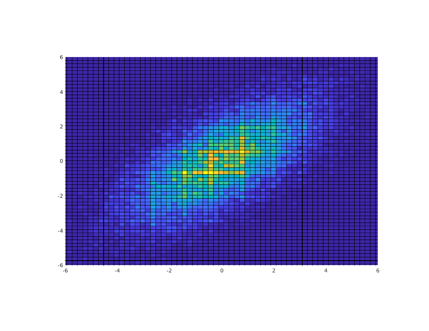
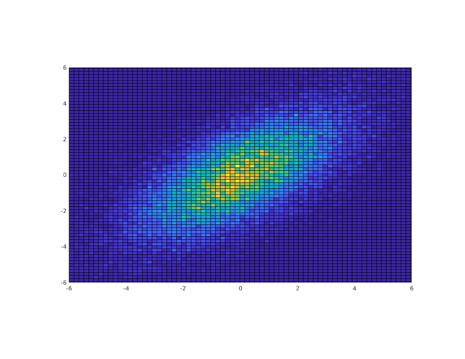
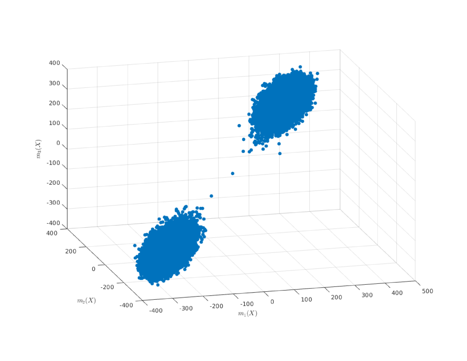
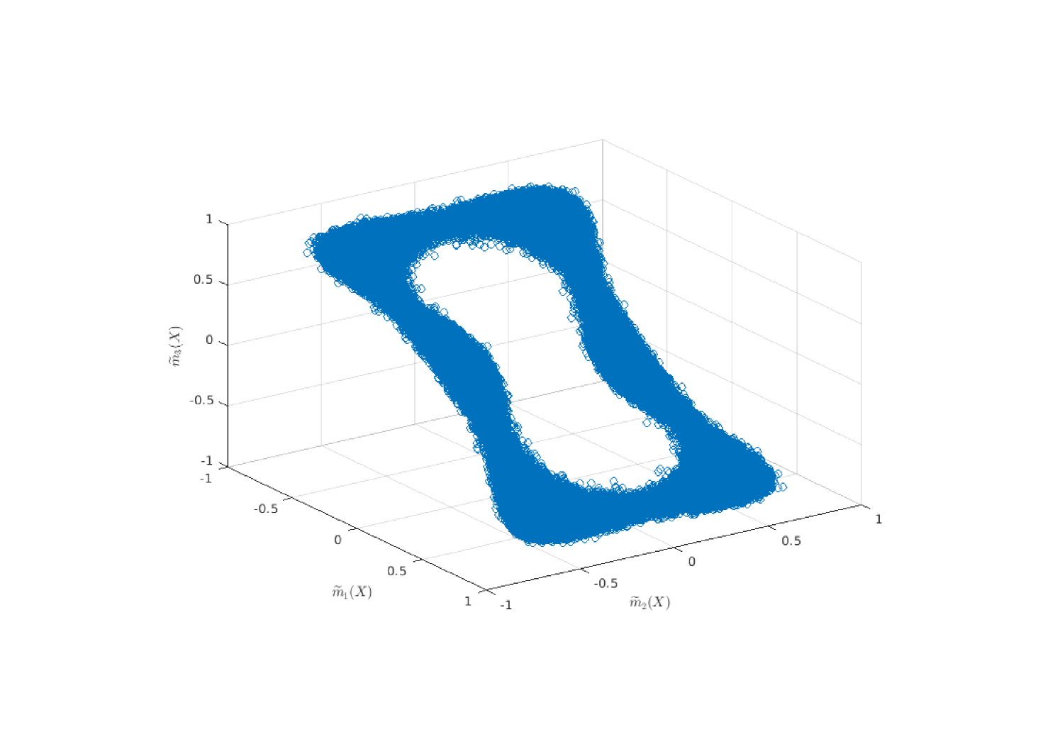
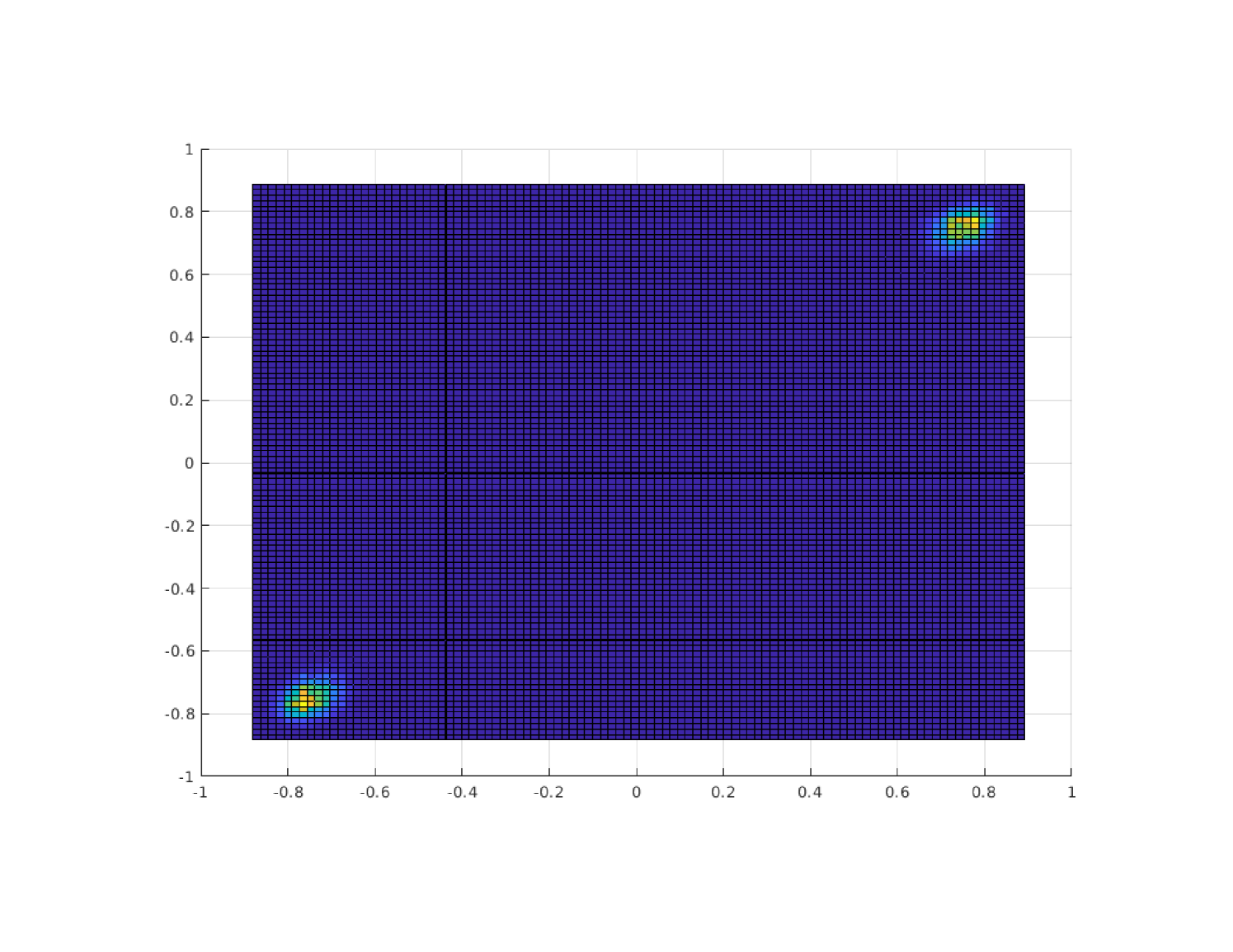
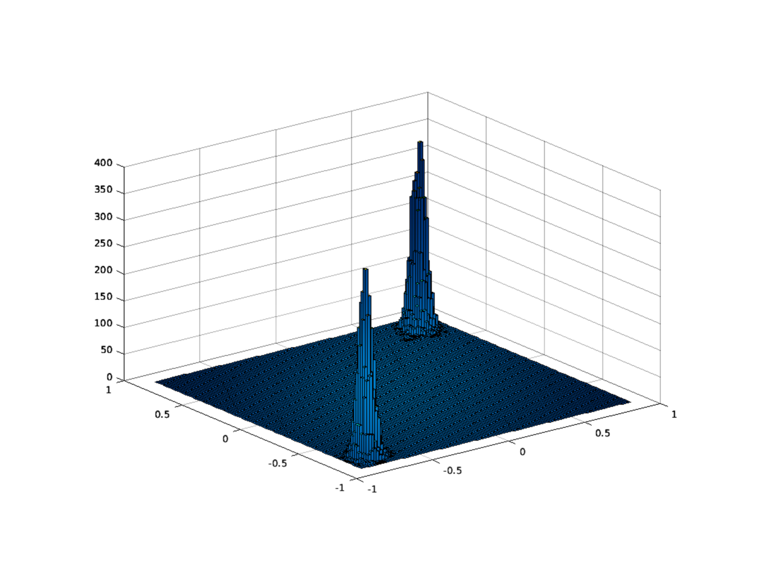
The first question concerns the maxima of the rate function II. Firstly, note that by [11, Theorem A.1] the global maxima of II are related to the global minima of the so-called pressure functional, which can for example be found in [17, equation (14)]. Using the compactness of [1,1]k[-1,1]^{k} and the continuity of II, the existence of a maximiser easily follows, but the number of maximisers is still obscure. From real-analyticity of II, we can infer that the set of maximisers is a λk\lambda^{k} null set, but it could in principle contain infinitely many points. However, Lemmas 2.5 and 2.6 as well as numerics suggest that for positive interactions and k2k\geq 2, the number of local minima is twice the number of independent systems - see Figures 2 for the k=3k=3 and 3 for the k=2k=2 case below.

However, we believe that the case of negative interactions between groups might drastically change the picture. Indeed, consider a model with three blocks and positive interaction β\beta within the blocks and negative interaction α\alpha between the blocks. Then, if β\beta is large enough, the points within the blocks will tend to be aligned. However, as α\alpha is negative, the magnetizations of block one and two will try to have different signs, but so do the magnetizations of blocks two and three, and three and one. Hence, frustration occurs. In this respect, a model with positive and negative interactions carries features of a spin glass.

Refer to caption
(a) Block interaction A=(20.90.70.920.40.70.42)A=\begin{pmatrix}2&0.9&0.7\\ 0.9&2&0.4\\ 0.7&0.4&2\end{pmatrix}
Refer to caption
(b) Block interaction A=(311131113)A=\begin{pmatrix}3&-1&-1\\ -1&3&-1\\ -1&-1&3\end{pmatrix}
Figure 2. A scatterplot of the normalized block magnetization m~\widetilde{m} in the uniform case with k=3k=3 blocks and n=500n=500, sampled using the Glauber dynamics – note that it is not rapidly mixing!
Refer to caption
Refer to caption
Figure 3. A heatmap (left) and a histogram (right) of the block magnetization vector m=(m1,m2)m=(m^{1},m^{2}) in the uniform, low temperature case. The block interaction matrix is given by A=(1.80.80.81.8)A=\begin{pmatrix}1.8&0.8\\ 0.8&1.8\end{pmatrix}.

Another question is the relationship of Theorems 1.3 and 1.5. In Theorem 1.5 we consider the distance to a normal distribution with covariance matrix Σn𝔼m^(n)(m^(n))T\Sigma_{n}\coloneqq\operatorname{\mathbb{E}}\hat{m}^{(n)}(\hat{m}^{(n)})^{T} and not to Σ(IdΓAΓ)1\Sigma_{\infty}\coloneqq(\operatorname{Id}-\Gamma_{\infty}A\Gamma_{\infty})^{-1}, which is the covariance matrix of the limiting distribution. Testing against functions h𝒞c(k)h\in\mathcal{C}_{c}^{\infty}(\operatorname{\mathbb{R}}^{k}), we see that Σ\Sigma_{\infty} is the limit of the matrices Σn\Sigma_{n}. It is an interesting task to provide suitable bounds of ΣnΣ\lVert\Sigma_{n}-\Sigma_{\infty}\rVert in any matrix norm, since [30, Proposition 2.8] provides bounds of |𝔼h(X)𝔼h(Y)|\lvert\operatorname{\mathbb{E}}h(X)-\operatorname{\mathbb{E}}h(Y)\rvert for two random vectors with X𝒩(0,Σ0)X\sim\mathcal{N}(0,\Sigma_{0}) and Y𝒩(0,Σ1)Y\sim\mathcal{N}(0,\Sigma_{1}) in terms of the 11-distance of Σ0\Sigma_{0} and Σ1\Sigma_{1}.

Thirdly, it remains an open problem to quantify the distance to a normal distribution with the “limiting” covariance matrix Σ\Sigma_{\infty}. The central limit theorem in the one-dimensional Curie–Weiss model has been solved for example in [14, Corollary 2.9]. Therein one can see that the limiting covariance is (1β)1(1-\beta)^{-1} by considering the approximate linear regression condition. A similar condition is true in the multidimensional case. For example, in Lemma 3.2 we have proven

(4.1) 𝔼(m^(n)m^(n))=λΛ1m^(n)+R(X),\operatorname{\mathbb{E}}\left(\hat{m}^{(n)}-\hat{m}^{(n)}\,{}^{\prime}\mid\mathcal{F}\right)=\lambda\Lambda^{-1}\hat{m}^{(n)}+R(X),

where λ=N1\lambda=N^{-1} and Λ=(IdΓnAΓn)1\Lambda=(\operatorname{Id}-\Gamma_{n}A\Gamma_{n})^{-1}. Thus, in the case ΓnΓ\Gamma_{n}\equiv\Gamma_{\infty} (e.g. consider a subsequence along which this holds) Λ\Lambda is the covariance matrix of the limit distribution. However, we have been unable to find a suitable modification of [30, Theorem 2.1] that enables one to compare the distribution of the random vector m^(n)\hat{m}^{(n)} with 𝒩(0,Λ)\mathcal{N}(0,\Lambda).

References

  • [1] E. Agliari, R. Burioni, and P. Contucci. A diffusive strategic dynamics for social systems. J. Stat. Phys., 139(3):478–491, 2010.
  • [2] A. A. Amini and E. Levina. On semidefinite relaxations for the block model. Ann. Statist., 46(1):149–179, 2018.
  • [3] Q. Berthet, P. Rigollet, and P. Srivastava. Exact recovery in the Ising blockmodel. Ann. Statist., 47(4):1805–1834, 2019.
  • [4] G. Bresler. Efficiently learning Ising models on arbitrary graphs [extended abstract]. In STOC’15—Proceedings of the 2015 ACM Symposium on Theory of Computing, pages 771–782. ACM, New York, 2015.
  • [5] G. Bresler, E. Mossel, and A. Sly. Reconstruction of Markov random fields from samples: some observations and algorithms. SIAM J. Comput., 42(2):563–578, 2013.
  • [6] W. A. Brock and S. N. Durlauf. Discrete choice with social interactions. Rev. Econom. Stud., 68(2):235–260, 2001.
  • [7] S. Chatterjee and Q.-M. Shao. Nonnormal approximation by Stein’s method of exchangeable pairs with application to the Curie-Weiss model. Ann. Appl. Probab., 21(2):464–483, 2011.
  • [8] F. Collet. Macroscopic limit of a bipartite Curie-Weiss model: a dynamical approach. J. Stat. Phys., 157(6):1301–1319, 2014.
  • [9] F. Comets. Large deviation estimates for a conditional probability distribution. Applications to random interaction Gibbs measures. Probab. Theory Related Fields, 80(3):407–432, 1989.
  • [10] R. Cont and M. Löwe. Social distance, heterogeneity and social interactions. J. Math. Econom., 46(4):572–590, 2010.
  • [11] M. Costeniuc, R. S. Ellis, and H. Touchette. Complete analysis of phase transitions and ensemble equivalence for the curie–weiss–potts model. J. Math. Phys., 46(6):063301, 2005.
  • [12] A. Dembo and O. Zeitouni. Large deviations techniques and applications, volume 38 of Stochastic Modelling and Applied Probability. Springer-Verlag, Berlin, 2010.
  • [13] F. den Hollander. Large deviations, volume 14 of Fields Institute Monographs. American Mathematical Society, Providence, RI, 2000.
  • [14] P. Eichelsbacher and M. Löwe. Stein’s method for dependent random variables occurring in statistical mechanics. Electron. J. Probab., 15:no. 30, 962–988, 2010.
  • [15] R. S. Ellis. Entropy, large deviations, and statistical mechanics. Classics in Mathematics. Springer-Verlag, Berlin, 2006.
  • [16] R. S. Ellis and C. M. Newman. Limit theorems for sums of dependent random variables occurring in statistical mechanics. Z. Wahrsch. Verw. Gebiete, 44(2):117–139, 1978.
  • [17] M. Fedele and P. Contucci. Scaling limits for multi-species statistical mechanics mean-field models. J. Stat. Phys., 144(6):1186–1205, 2011.
  • [18] M. Fedele and F. Unguendoli. Rigorous results on the bipartite mean-field model. J. Phys. A, 45(38):385001, 18, 2012.
  • [19] I. Gallo, A. Barra, and P. Contucci. Parameter evaluation of a simple mean-field model of social interaction. Math. Models Methods Appl. Sci., 19(suppl.):1427–1439, 2009.
  • [20] I. Gallo and P. Contucci. Bipartite mean field spin systems. Existence and solution. Math. Phys. Electron. J., 14:Paper 1, 21, 2008.
  • [21] C. Gao, Z. Ma, A. Y. Zhang, and H. H. Zhou. Achieving optimal misclassification proportion in stochastic block models. J. Mach. Learn. Res., 18:Paper No. 60, 45, 2017.
  • [22] B. Gentz and M. Löwe. The fluctuations of the overlap in the Hopfield model with finitely many patterns at the critical temperature. Probab. Theory Related Fields, 115(3):357–381, 1999.
  • [23] F. Götze, H. Sambale, and A. Sinulis. Higher order concentration for functions of weakly dependent random variables. Electron. J. Probab., 24:no. 85, 19 pp, 2019.
  • [24] J. M. Kincaid and E. G. D. Cohen. Phase diagrams of liquid helium mixtures and metamagnets: Experiment and mean field theory. Physics Reports, 22(2):57 – 143, 1975.
  • [25] W. Kirsch and G. Toth. Two groups in a Curie-Weiss model with heterogeneous coupling. Journal of Theoretical Probability, 2019.
  • [26] H. Knöpfel and M. Löwe. Zur Meinungsbildung in einer heterogenen Bevölkerung—ein neuer Zugang zum Hopfield Modell. Math. Semesterber., 56(1):15–38, 2009.
  • [27] M. Löwe and K. Schubert. Fluctuations for block spin Ising models. Electron. Commun. Probab., 23:Paper No. 53, 12, 2018.
  • [28] E. Mossel, J. Neeman, and A. Sly. Belief propagation, robust reconstruction and optimal recovery of block models. Ann. Appl. Probab., 26(4):2211–2256, 2016.
  • [29] A. A. Opoku, K. Owusu Edusei, and R. K. Ansah. A conditional Curie-Weiss model for stylized multi-group binary choice with social interaction. J. Stat. Phys., 171(1):106–126, 2018.
  • [30] G. Reinert and A. Röllin. Multivariate normal approximation with stein’s method of exchangeable pairs under a general linearity condition. Ann. Probab., 37(6):2150–2173, 2009.
  • [31] J. L. van Hemmen, D. Grensing, A. Huber, and R. Kühn. Elementary solution of classical spin-glass models. Z. Phys. B, 65(1):53–63, 1986.
  • [32] J. L. van Hemmen, A. C. D. van Enter, and J. Canisius. On a classical spin glass model. Z. Phys. B, 50(4):311–336, 1983.