Fluctuations of particle systems determined by Schur generating functions
Abstract.
We develop a new toolbox for the analysis of the global behavior of stochastic discrete particle systems. We introduce and study the notion of the Schur generating function of a random discrete configuration. Our main result provides a Central Limit Theorem (CLT) for such a configuration given certain conditions on the Schur generating function. As applications of this approach, we prove CLT’s for several probabilistic models coming from asymptotic representation theory and statistical physics, including random lozenge and domino tilings, non-intersecting random walks, decompositions of tensor products of representations of unitary groups.
1. Introduction
1.1. Overview
This article is about the random –particle configurations on and their asymptotic behavior as . For each let be a random –dimensional vector
| (1.1) |
Our aim is to deal with global fluctuations of . One way to make sense of those is to take an arbitrary test function and consider linear statistics
| (1.2) |
We mostly deal with the case when is a polynomial (or, more generally, a smooth function), yet if is the indicator function of an interval, then (1.2) merely counts the number of random particles inside this interval.
Since by its definition, is a sum of terms, it is reasonable to expect that it grows linearly in . And, indeed, in the class of systems that we study, converges as to a deterministic limit depending on the choice of . We will refer to such a phenomenon as the Law of Large Numbers, appealing to the evident analogy with a similar statement of classical probability dealing with sequences of independent random variables.
The next natural question is to study the fluctuations as . Such fluctuations would grow as in the systems arising from sequences of independent random variables, but the scale is different in our context. We deal with probability distributions coming from statistical mechanics (lozenge and domino tilings, families of non-intersecting paths), asymptotic representation theory, random matrix theory, and for them the typical situation is that does not grow as . Nevertheless, in all cases the fluctuations are asymptotically Gaussian, which justifies the name Central Limit Theorem for these kinds of results.
The main theme of the present article is to develop a new toolbox for proving the Law of Large Numbers and Central Limit Theorems, which would be robust to perturbations of . It is somewhat hard to concisely describe the class of systems where the toolbox is helpful. One reason is that we believe our conditions to be in a sense equivalent to the LLN and CLT, see the end of Section 1.4 (which, of course, does not make these conditions immediate to check). Yet we list below an extensive list of available applications.
Again coming back to the classical one-dimensional probability, a universal tool is given there by the method of characteristic functions. For instance, it can be used to prove that averages of independent random variables converge to a Gaussian limit under very mild assumptions on the distributions of these variables, cf. textbooks [Ka], [Dur].
In our context the characteristic functions were not found to be useful, mostly due to the fact that the dimension (number of the particles) grows with , while the individual coordinates , are very far from being independent. Therefore, we suggest to replace them by a new notion of Schur generating function which we now introduce.
Recall that a Schur function is a symmetric Laurent polynomial in variables parameterized by and given by
Let denote the –tuple and note that the map makes the weakly decreasing coordinates of strictly decreasing, as in (1.1).
For a random –tuple of strictly ordered integers , as in (1.1), its distribution is a function of weakly decreasing integers given by .
Definition 1.1.
The Schur generating function of a random –distributed –particle configuration , is a function of variables given by
| (1.3) |
In [BuG] we showed how the Law of Large Numbers can be extracted from the asymptotic behavior of Schur generating functions. Interestingly, the answer, i.e. the exact formula for depends only on and the asymptotics of , that is, all variables except for one can be set to prior to the asymptotic analysis. A similar phenomenon was also found in [MN] by another method.
Here we make the next step and address the Central Limit Theorem for global fluctuations, the precise statement in this direction is Theorem 2.8. In fact, we go even further, and also analyze random sequences of –particle configurations forming Markov chains, see Theorems 2.9, 2.10, 2.11 below. This time the answer, which is the covariance for , depends only on asymptotics of , that is, all variables except for two can be set to prior to the asymptotic analysis. For proving the asymptotic Gaussianity we need more.
Our theorems reduce the LLN and CLT to asymptotic behavior of Schur generating functions, which is known in many cases. This leads to proofs of the LLN and CLT for a variety of stochastic systems of particles, including:
- (1)
- (2)
- (3)
-
(4)
–dimensional random growth models.
-
(5)
Measures governing the decomposition into irreducible components for tensor products of irreducible representations of the unitary group .
-
(6)
Measures governing the decomposition of restrictions onto of extreme characters of the infinite–dimensional unitary group .
-
(7)
Schur–Weyl measures.
A more detailed exposition of the applications of our method is given in Section 3.
1.2. Previous work on the subject
One advantage of our approach through Schur generating functions is that it is quite general, and as a result, in each of our applications we can address more general situations than those rigorously known before. However, particular cases of some of our applications were accessible previously by other important techniques. Let us list several of those.
-
•
Determinantal point processes have led to Central Limit Theorems for uniformly random lozenge tilings of certain domains in [Ken], [Pet2], for dimensional random growth in [BF], [Dui1], [Ku1]. Similar results for domino tilings of the Aztec diamond were announced (without technical details) in [CJY].
- •
-
•
Discrete loop equations (also known as Nekrasov equations) have led in [BGG] to Central Limit Theorems for discrete log–gases, which has overlaps with specific ensembles of non-intersecting paths and tilings.
-
•
Various representation–theoretic ideas, involving, in particular, computations in the algebra of shifted symmetric functions and universal enveloping algebra of have led in [Ker], [IO], [F], [HO], [BBu], [BBO], [DF], [Ku2], [Mel] to several instances of Central Limit Theorem for the probability distributions of asymptotic representation theory.
-
•
Differential operators acting in the algebra of symmetric functions in infinitely-many variables were used in [Mo] for proving the Central Limit Theorem for the Jack measures.
Let us emphasize, that despite the existence of several competing methods, most of our applications were not previously accessible by any of them. Yet our technique is adapted to the study of the global behavior of probabilistic systems, while some of these methods are more suitable for the study of the local behavior.
1.3. Continuous models
Replacing by in (1.1), we arrive at continuous analogues of the particle configurations under consideration. In this fashion, our results are closely related to the global asymptotics for the eigenvalues of random matrix ensembles.
One precise example is given by the semiclassical limit, which degenerates the decomposition of tensor products of irreducible representations of (one of our applications) to spectral decomposition of sums of independent Hermitian matrices, see [BuG, Section 1.3] for the details. The Central Limit Theorem for this random matrix problem is well-known, see [PS, Section 10]. It can be put into the context of the second order freeness in the free probability theory, see [MS], [MSS]. In Section 9.4 we explain how the covariance for our Central Limit Theorem for tensor products degenerates to the random matrix one.
Another degeneration is the appearance of the Gaussian Unitary Ensemble (GUE) as a scaling limit of lozenge and domino tilings near the boundary of the tiled domain, see [OR], [JN], [GP], [No]. Recall that GUE is the eigenvalue distribution of , where is matrix of i.i.d. mean complex Gaussian random variables. And again for GUE the Gaussian asymptotics for global fluctuations is well–known and can be generalized in (at least) two directions. The first one is a general Central Limit Theorem for (continous) log–gases of [J1] based on the loop equations. The second generalization is to replace the Gaussian distributions in the definition of GUE by arbitrary ones and to study the resulting Wigner matrix. Then the global fluctuations can be accessed by the moments method, see e.g. [AGZ, Chapter 2] for an exposition. In more details, one computes the moments of the eigenvalues in the following form
| (1.4) |
The independence of matrix elements of paves a way to find the asymptotic of the left–hand side of (1.4), which then gives the global asymptotic of linear statistics of the form (1.2) with polynomial test functions .
1.4. Moments method
The moments method was never available for the discrete particle configurations as in (1.1) for a very simple reason: there is no underlying random matrix or an analogue thereof. Here we change this situation by providing a way to efficiently compute (a discrete analogue of) the right–hand side in (1.4). Let us briefly state the key idea.
Let denote the derivative with respect to the variable and consider the differential operator
A straightforward computation shows that the Schur functions are eigenvectors of :
Therefore, applying such operators to (1.3) we get
| (1.5) |
The fact that differential (or difference) operators applied to symmetric functions can be used for the analysis of random particle configurations is by no means new, see e.g. [BC], [BCGS] for recent similar statements, and the asymptotic questions boil down to finding a way to analyze the right–hand side of (1.5). This is where the specific and relatively simple definition of shines, as we are able to develop a combinatorial approach (yet based on several analytic lemmas) to the right–hand side of (1.5).
One important observed feature is that the right–hand side of (1.5) depends only on the values of the Schur generating function at points such that all but a bounded number of coordinates (i.e. the total number is not growing with ) are equal to . First, this reduces a problem in growing (with ) dimension to a much more tractable finite–dimensional form. Second, the values of Schur generating functions at such points are very robust and not too sensitive to small perturbations for . This is indicated by the results of [GM], [GP] on the asymptotics of Schur functions, on which we elaborate in Section 8. In particular, these results give enough control on the values of Schur generating functions to give the asymptotic expansion for the left–hand side of (1.5) needed for the Central Limit theorem. In contrast to our method, previous results and related approaches in the area, such as those of [BBu], [BC], [BCGS], [BBO], [Mo] relied on the exact form of the Schur generating function or its analogue; in particular, it was necessary to assume its factorization into a product of –variable functions.
From the technical point of view, even after all these observations are made, the asymptotic analysis still needs many efforts and is much more complicated than that of [BuG] where the Law of Large Numbers was addressed through the same technique.
Let us end this section with a speculation. We believe that it should be possible to reverse the theorems of the present article: the knowledge of the Law of Large Numbers and Central Limit Theorem should give (perhaps, subject to technical conditions) exhaustive information about asymptotics of the Schur generating functions for all but finitely many values of coordinates equal to . We plan to develop this direction in a separate publication111This was subsequently proven to be true, see [BuG2]..
1.5. Organization of the article
The rest of the text is organized as follows. In Section 2 we formulate our main results linking the Central Limit Theorem for global fluctuations to the asymptotic of Schur generating functions. Numerous applications of these results are presented in Section 3. Section 4 gives a generalization of (1.5) which underlies all our developments. The remaining sections present a step-by-step proof for the statements of Sections 2 and 3.
1.6. Acknowledgements
We would like to thank Alisa Knizel for help with preparing the picture of a domino tiling. We thank Alexei Borodin for useful comments. We are grateful to an anonymous referee for suggestions on improving the text. V.G. was partially supported by the NSF grant DMS-1407562, by the NEC Corporation Fund for Research in Computers and Communications and by the Sloan Research Fellowship. Both authors were partially supported by the NSF grant DMS-1664619.
1.7. Notation
Here we collect some notations that we use throughout this paper. Note that some of these notations are slightly unconventional.
By we denote the variables .
We denote by the sequence .
By we denote the partial derivative . We use instead of . For a function of one variable we sometimes denote the derivative by the conventional notation . By we mean the function itself.
For a differential operator by we mean that the differential operator is applied to only. Let be the group of all permutations of elements; then
denotes the symmetrization of a function.
Let be the Vandermond determinant in variables .
Sometimes we omit the arguments of functions in formulas. For example, we can use the symbol instead of .
We use notations , .
denotes the summation over all subsets of consisting of elements.
All contours of integration in this paper are counter-clockwise.
2. Main results
2.1. Preliminaries and Law of Large Numbers
An -tuple of non-increasing integers is called a signature of length . We denote by the set of all signatures of length . The Schur function , , is a symmetric Laurent polynomial defined by
Let be a probability measure on the set . A Schur generating function is a symmetric Laurent power series in given by
In what follows we always assume that the measure is such that this (in principle, formal) sum is uniformly convergent in an open neighborhood of . Note that the uniform convergence of such a series in a neighborhood of implies the uniform convergence in an open neighborhood of the -dimensional torus . Indeed, it follows from the estimate (which is an immediate corollary of the combinatorial formula for Schur functions as a positive sum of monomials, see [Ma, Chapter I, Section 5, (5.12)]).
The goal of this paper is to show how to extract information about with the help of .
Definition 2.1.
A sequence of symmetric functions is called LLN-appropriate if there exists a collection of reals such that
-
•
For any the function is holomorphic in an open complex neighborhood of .
-
•
For any index and any we have
-
•
For any and any indices such that there are at least two distinct indices among them we have
-
•
The power series
converges in a neighborhood of the unity.
Definition 2.2.
A sequence , where is a probability measure on , is called LLN-appropriate if the sequence of its Schur generating functions is LLN-appropriate. For such a sequence we define a function via
where are the coefficients from Definition 2.1.
General Example 2.3.
Assume that the Schur generating functions of a sequence of probability measures , where is a probability measure on , satisfies the condition
where is a holomorphic function, and the convergence is uniform in a complex neighborhood of . Then is a LLN-appropriate sequence with .
Indeed, for a uniform limit of holomorphic functions the order of taking derivatives and limit can be interchanged, which shows that the example above is correct. In applications studied in this paper all LLN-appropriate measures will come from the construction of Example 2.3. However, we prefer to prove general theorems in a slightly more general setting of Definition 2.2.
For a signature consider the measure on
| (2.1) |
The pushforward of a measure on with respect to the map defines a random probability measure on which we denote by .
The following theorem is essentially [BuG, Theorem 5.1]. In Section 10 we comment on the slight difference between this formulation and the one given in [BuG].
Theorem 2.4.
Suppose that a sequence of probability measures , where is a probability measure on , is LLN-appropriate, and . Then the random measures converge as in probability, in the sense of moments to a deterministic measure on , such that its th moment equals
| (2.2) |
where .
2.2. Main result: CLT for one level
Definition 2.5.
We say that a sequence of symmetric functions is appropriate (or CLT-appropriate) if there exist two collections of reals , , such that
-
•
For any the function is holomorphic in an open complex neighborhood of .
-
•
For any index and any we have
-
•
For any distinct indices and any we have
-
•
For any and any indices such that there are at least three distinct numbers among them we have
-
•
The power series
converge in an open neighborhood of and , respectively.
Definition 2.6.
We say that a sequence of measures is appropriate (or CLT-appropriate) if the sequence of its Schur generating functions is appropriate. For such a sequence we define functions
General Example 2.7.
Assume that the Schur generating function of a sequence of probability measures on satisfies the conditions
where are holomorphic functions, and the convergence is uniform in a complex neighborhood of unity. Then is a (CLT-)appropriate sequence of measures with , .
Indeed, for a uniform limit of holomorphic functions the order of taking derivatives and limit can be interchanged, which shows that the example above is correct. In applications studied in this paper all CLT-appropriate measures will come from the construction of Example 2.7. However, we prefer to prove theorems for a slightly more general setting of Definition 2.6.
Let be a probability measure on . Set
The following theorem is the main result of this paper.
Theorem 2.8.
Let be an appropriate sequence of measures on signatures with limiting functions and (see Definition 2.6).
Then the collection
converges, as , in the sense of moments, to the Gaussian vector with zero mean and covariance
where the - and -contours of integration are counter-clockwise and .
This theorem serves as a model example of our approach. However, for applications it is often required to study the joint distributions of several random particle systems. Our approach can be applied to (some of) these cases as well: We deal with them in the next sections.
2.3. General setting for several levels
Let us introduce a general construction of Markov chains which are analyzable by our methods.
For a positive integer and let be the space of analytic symmetric functions in the region
We consider as a topological space with topology of uniform convergence in this region.
Consider endowed with the topology of the inductive limit. Note that for the function is an (antisymmetric) analytic function. Therefore, it can be written as an absolutely convergent sum of monomials , where , . Dividing both sides of such a sum by , we obtain that each element of can be written in a unique way as an absolutely convergent sum
in some neighborhood of the -dimensional torus.
We consider a map with the following properties:
1) is a linear continuous map.
2) For every we have
This property says that the coefficients must be nonnegative reals (rather than arbitrary complex numbers). Note that the sum in the right-hand side is absolutely convergent due to the definition of .
3) For any we have
In words, this property asserts that our map should preserve the value at unity.
It follows from conditions 2) and 3) that
Since these coefficients are nonnegative reals one can consider them as transitional probabilities of a Markov chain. In more details, let be positive integers, and let , …, be maps satisfying conditions above. Let be a probability measure on . Define the probability measure on the set
via
| (2.3) |
In Section 4 we prove a formula for the expectation of joint moments of signatures distributed according to this measure.
2.4. Main result: CLT for several levels
In this section we state three multi-level generalisations of Theorem 2.8. They are mainly shaped to the applications studied in the present paper. With the use of the construction from Section 2.3 it is possible to produce many other similar multi-level generalisations of Theorem 2.8; this should be regulated by applications that one has in mind.
We consider the following particular examples of the map from Section 2.3. In the first case, it is given by , for . In the second case, it is given by , for and a function which is a Schur generating function of a probability measure on . Finally, in the third case we combine the two previous ones.
In an attempt to make the exposition more explicit, we repeat the construction of Section 2.3 in all three cases below.
Example 1) For , with , let us introduce the coefficients via
| (2.4) |
The branching rule for Schur functions asserts that the coefficients are non-negative for all , (see [Ma, Chapter 1.5]). Plugging in , we see that .
Let be fixed positive reals, and let be a probability measure on .
Let us introduce the probability measure on the set via
| (2.5) |
(the fact that all these weights are summed up to can be straightforwardly checked by induction over .)
We are interested in the joint distributions of random signatures of this random array. For , let be a (shifted) power sum of coordinates of signatures defined by the formula
where is distributed according to the measure (2.5).
Theorem 2.9.
Assume that is an appropriate sequence of probability measures on , , in the sense of Definition 2.6 and corresponding to functions and . Let us consider the probability measure on the sets of signatures defined by (2.5). In the notations above, the collection of random variables
converges, as , in the sense of moments, to the Gaussian vector with zero mean and covariance:
where and .
Example 2) Let us start with the following classical fact. For there is a decomposition of the product of two Schur functions into a linear combination of Schur functions:
| (2.6) |
The coefficients are well-known under the name of Littlewood-Richardson coefficients. It is known that for arbitrary they are nonnegative (see, e.g., [Ma, Chapter 1.9]).
Let , , , …, be sequences of appropriate measures, where , , …, are probability measures on . Let be the Schur generating functions of , , …, , respectively.
Define the coefficients , for , , , via
| (2.7) |
Note that the series in the right-hand side is absolutely convergent and the coefficients are nonnegative. Using (2.6), one can write an explicit formula for them:
Let us define a probability measure on the set
| (2.8) |
We define the probability of the configuration
via
| (2.9) |
Let be the th shifted power sum of :
Let
| (2.10) |
It can be directly shown by induction that the functions , are Schur generating functions of , . Moreover, they are appropriate (in the sense of Definition 2.5) because and are appropriate sequences of functions.
Let us denote the corresponding to limit functions from Definition 2.6 by , , and .
Theorem 2.10.
Assume that , , , …, are appropriate sequences of probability measures, and let , , , , , , , be as above. Then the collection of random variables
converges, in the sense of moments, to the Gaussian vector with zero mean and covariance:
| (2.11) |
where and .
Example 3) Now let us turn to a case which unites the two previous ones. Let be a positive integer and let be reals. Let , , …, , be appropriate sequences of probability measures such that is a probability measure on . Let , , , be Schur generating functions of , , …, , , respectively.
Define the coefficients , for , , , via
| (2.12) |
Note that the series in the right-hand side is absolutely convergent and the coefficients are nonnegative. Using (2.4) and (2.6), one can write an explicit formula for them:
In this definition we combine two operations on appropriate Schur generating functions which we use in the two previous cases: The substitution of ’s into some variables and multiplication by a function.
Let us define the probability measure on the set
That is, we want to define the probability of a collection of signatures
where is a signature of length , . Let us do this in the following way. We define this probability via
| (2.13) |
Let be the th shifted power sum of :
Let
It can be directly shown by induction that the functions , are Schur generating functions of , . Moreover, they are appropriate (in the sense of Definition 2.5) because and are appropriate sequences of functions. Let us denote the corresponding limit functions by , , , for .
Theorem 2.11.
In the notations above, the collection of random functions
is asymtoticaly Gaussian with the limit covariance
where and .
3. Applications
In this section we state several applications of general theorems from Sections 2.2 and 2.4. The theorems are split into two parts: Sections 3.2, 3.4 are devoted to problems of asymptotic representation theory, while Sections 3.5, 3.6, 3.7 deal with 2d lattice models of statistical mechanics.
3.1. Preliminary definitions
In a considerable part of our theorems an input is given by a sequence , of signatures. Depending on the context, they encode irreducible representations, boundary conditions in statistical mechanics models or initial conditions of Markov chains.
In our asymptotic results we are going to make the following technical assumption on the behavior of as becomes large.
Definition 3.1.
A sequence of signatures is called regular, if there exists a piecewise–continuous function and a constant such that
| (3.1) |
and
| (3.2) |
Remark 3.2.
Informally, the condition (3.1) means that scaled by coordinates of approach a limit profile . The restriction that is piecewise–continuous is reasonable, since is a limit of monotonous functions and, thus, is monotonous (therefore, we only exclude the case of countably many points of discontinuity for ). This restriction originates in the asymptotic results of [GP] and we believe that it, in fact, can be weakened for most applications, cf. [No], [MN].
It is clear that if the sequence is regular, then the sequence (defined by (2.1)) weakly converges to a probabilistic measure on with compact support. The complete information about such measure can be encoded in several generating functions that we now define.
For a probability measure on with compact support let us define the Cauchy-Stieltjes transform by
| (3.3) |
This is a power series in which converges in a neighborhood of infinity.
Define to be the inverse series to , i.e. such that
(As a power series has a form ). Further, set
| (3.4) |
The function is well-known in the free probability theory under the name of Voiculescu –transform, cf. [VDN], [NS].
Integrating , set
which should be understood as a holomorphic function in a neighborhood of .
The derivative of has a simpler form:
| (3.5) |
The function plays an important role in the context of the quantized free convolution, see [BuG].
3.2. Asymptotic decompositions of representations of
Here we briefly recall some facts about representations of the unitary group (see e.g. [FH], [W], [Zh]) and state a central limit theorem for decompositions of their tensor products and restrictions.
Let be the group of all unitary matrices. It is a classical fact that the irreducible representations of are parameterized by signatures of length . Let us denote by the irreducible representation of corresponding to the signature ( is the highest weight of this representation), and let denote the dimension of this representation.
Consider a reducible finite-dimensional representation of and let
be a decomposition of into irreducibles.
One of the basic ideas of asymptotic representation theory is to associate with a probability measure on the set of labels of irreducible representations. In the case of the unitary group this results into the definition of the probability measure :
| (3.6) |
We reduce the study of the asymptotic behavior of such probability measures to their moments defined through
| (3.7) |
One basic operation which creates reducible representations is tensor product. The decomposition of the (Kronecker) tensor product into irreducibles can be written with the use of classical Littlewood-Richardson coefficients :
with an equivalent definition being (2.6). The Law of Large Numbers for tensor products was proven in [BuG], and here is the Central Limit Theorem.
For two probability measures and with compact support set
| (3.8) |
Theorem 3.3 (Central Limit Theorem for tensor products).
Remark 3.4.
In this setting the operation of the tensor product of representations can be seen as a quantization of the summation of independent random matrices. The degeneration from representations to matrices is known as a semiclassical limit, see e.g. [BuG, Section 1.3] and references therein for details. Under this limit transition Theorem 3.3 turns into the result for the spectra of the sum of the Haar-distributed random Hermitian matrices with a fixed spectrum. In Section 9.4 we show that in this limit the covariance (3.9) turns into the covariance for the random matrix problem, which can be found in [PS].
Remark 3.5.
In a similar way one can prove a central limit theorem for decomposition of for arbitrary positive integer .
Remark 3.6.
There is an approach to decomposition of tensor products via Perelomov-Popov measures, see [BuG] for details. In this setting, one obtains a direct relation of these measures and free probability. It would be interesting to relate Theorem 3.3 and the concept of second-order freeness developed in [MS], [MSS].
Proof of Theorem 3.3.
We believe that Theorem 3.3 is new. Yet, there are simpler tensor products whose asymptotic decomposition were intensively studied before in the context of the Schur–Weyl duality, cf. [Bi],[Mel]. For that consider a representation of in vector space via , . The decomposition of into irreducibles is governed by the Schur–Weyl measure, while its limit (when is kept fixed) is the celebrated Plancherel measure of the symmetric group .
Theorem 3.7 (Central Limit Theorem for Schur–Weyl measures).
Assume that for and let , . Then, as , the random vector of moments (3.7)
converges, in the sense of moments, to the Gaussian vector with zero mean and covariance
| (3.10) |
where .
Proof.
It is easy to see that the Schur generating function of is given by the normalized character of this representation:
We have
It remains to use Theorem 2.8. ∎
An earlier proof of Theorem 3.7 is given in [Mel], while its version is the Kerov’s Central Limit Theorem for the Plancherel measure, see [Ker], [IO].
Another natural operation on representations of is restriction onto the subgroup , where is identified with the subgroup of fixing the last coordinate vectors.
Theorem 3.8 (Central Limit Theorem for restrictions).
Suppose that , , is a regular sequence of signatures such that
Take and let be a representation of given by . Then, as , the random vector of moments (3.7)
converges, in the sense of moments, to the Gaussian vector with zero mean and covariance
| (3.11) |
where and function was defined in Section 3.1.
3.3. Preliminaries: Gaussian Free Field
A Gaussian family is a collection of Gaussian random variables indexed by an arbitrary set . We assume that all our random variables are centered, i.e.
Any Gaussian family gives rise to a covariance kernel defined by
Assume that a function is such that for any and , is a symmetric and positive-definite matrix. Then (see e.g. [C]) there exists a centered Gaussian family with the covariance kernel .
Let be the upper half-plane, and let be the space of smooth real–valued compactly supported test functions on . Let us set
and define a covariance kernel via
The Gaussian Free Field (GFF) on with zero boundary conditions can be defined as a Gaussian family with covariance kernel . The field cannot be defined as a random function on , but one can make sense of the integrals over finite contours in with continuous functions , see [Sh], [Dub, Section 4], [HMP, Section 2] for more details.
In our results GFF will play a role of the universal limit object for two-dimensional fluctuations of probabilistic models under consideration. In this sense, GFF plays a similar role to Brownian motion and Gaussian distribution.
3.4. Extreme characters of
In this section we switch from to its infinite–dimensional version. Consider the tower of embedded unitary groups
where is embedded into as the subgroup fixing the last coordinate vector. The infinite–dimensional unitary group is the inductive limit of these groups:
Define a character of the group as a continuous function that satisfies the following conditions:
-
•
, where is the identity element of (normalization);
-
•
, where are any elements of (centrality);
-
•
is an Hermitian and positive-definite matrix for any and (positive-definiteness);
The space of characters of is obviously convex. The extreme points of this space are called extreme characters; they replace characters of irreducible representations in this infinite-dimensional setting. The classification of the extreme characters of is known as the Edrei–Voiculescu theorem (see [Vo], [E], [VK], [OO], [BO]). It turns out that the extreme characters can be parameterized by the set , where
Each gives rise to a function via
| (3.12) |
Then the extreme character of corresponding to is given by
(this product is essentially finite, because only finitely many of ’s are distinct from ).
Each character gives rise to a probabilistic object known as the central measure on the Gelfand–Tsetlin graph. Let us present the necessary definitions.
The Gelfand-Tsetlin graph is defined by specifying its set of vertices as and putting an edge between any two signatures and such that they interlace , which means
We agree that consists of a single empty signature joined by an edge with each vertex of . A path between signatures and , , is a sequence
An infinite path is a sequence
We denote by the set of all paths starting in and of length . We denote by the set of all infinite paths.
For any character of one can associate a probability measure on paths . Indeed, for any fixed let us define a probability measure on via the linear decomposition
Next, define a weight of a subset of consisting of all paths with prescribed members up to by
| (3.13) |
Note that this weight depends on only. It can be easily deduced from the branching rules for characters of that this definition is consistent and correctly defines a probability measure on .
We will analyze the asymptotics of probability measures corresponding to certain sequences of extreme characters
In more detail, we will assume that a sequence satisfies the following condition.
Condition. We will consider sequences such that, as , we have
| (3.14) |
where , , , are arbitrary finite (not necessarily probability) measures on with compact support, are two positive real numbers, and we consider the convergence of finite measures in the weak sense. We will denote by the sextuple , , , which consists of 4 finite measures and 2 real numbers.
A direct computation shows that if a sequence satisfies the condition (3.14), then we have the following convergence of the Voiculescu functions (3.12)
| (3.15) |
where is determined by with the use of the formula (9.7); we do not need the explicit formula for it at this moment.
The description of CLT for extreme characters involves the following functions.
Proposition 3.9.
Let be the function which is obtained in the limit (3.15). For any and the equation
has at most one root . Let be the set of pairs such that this root exists. Then the map from such a pair to such a root is a diffeomorphism.
We prove this proposition in Section 9.2.
Let be an inverse of the map given by Proposition 3.9. Proposition 3.9 introduces coordinates in which the fluctuations of extreme characters become a Gaussian Free Field.
In order to make this statement precise, let us introduce the height function given by the formula
| (3.16) |
where are the coordinates of the signature from in the path which belongs to .
Let us equip with a probability measure , where satisfies the condition (3.15). Then becomes a random function which describes a certain random stepped surface.
Let us carry over to through
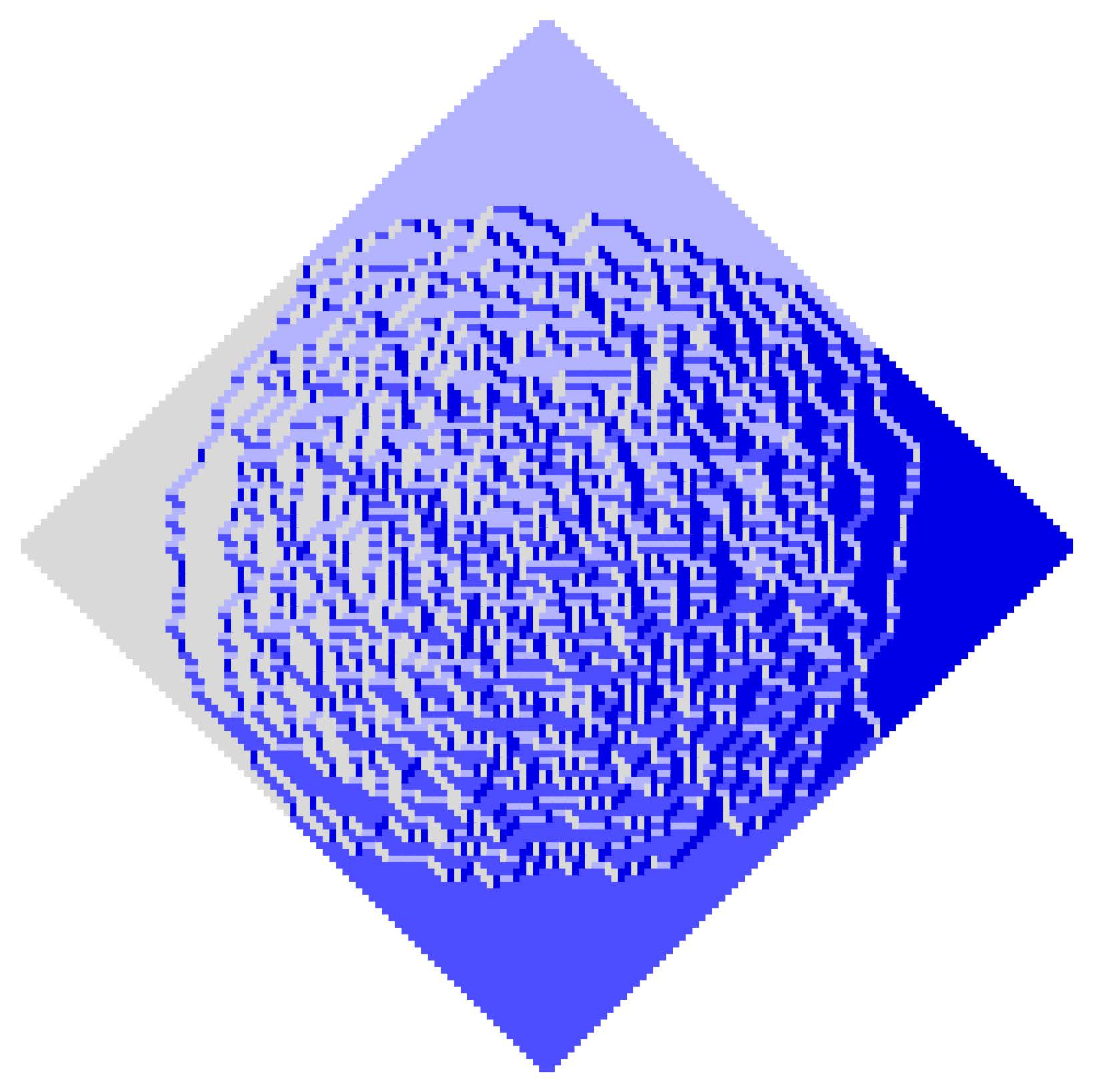
One might worry that some information is lost in this transformation, as the image of the map is smaller than , yet the configuration is actually frozen outside this image and there are no fluctuations to study, cf. Figures 2, 3, where random tilings are frozen outside inscribed circles.
For and define a moment of the random height function as
Also define the corresponding moment of GFF via
Theorem 3.10 (Central Limit Theorem for extreme characters).
Assume that the sequence of extreme characters satisfies condition (3.14). Let be a random height function on corresponding to as above. Then
In more details, as , the collection of random variables converges, in the sense of moments, to .
Remark 3.11.
For explicit expressions for the covariance of see (9.14).
Remark 3.12.
The condition (3.14) for the growth of extreme characters was introduced and studied in [BBO], where the law of large numbers for this probabilistic model was proven. Among other connections, the condition (3.14) is related to the hydrodynamical limit of random surfaces related to probabilistic particle systems with local interaction, see Section 3.3 of [BBO] for more details.
The proof of Theorem 3.10 is given in Section 9.2. We believe that this statement is new for general extreme characters. For the very special case when the only non-zero parameter in (3.14) is it was previously proven in [BF], [BBu].
The paths of and can be identified with lozenge tilings, which leads us to statistical mechanics applications.
3.5. Lozenge tilings
Consider a (right) halfplane on the regular triangular lattice. We would like to
tile this halfplane with lozenges (rhombuses) of three types: horizontal
![]() , and two others
, and two others
![]() ,
,
![]() . Let
denote the set of complete tilings of the half–plane subject to two boundary
conditions: the lozenges become
. Let
denote the set of complete tilings of the half–plane subject to two boundary
conditions: the lozenges become
![]() as one goes far up and
as one goes far up and
![]() as one goes far down, see
Figure 1.
as one goes far down, see
Figure 1.
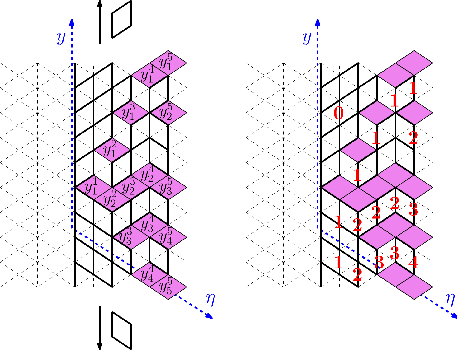
There is a natural bijection between and the set of paths in the Gelfand–Tsetlin graph. For that observe that due to combinatorial constraints, there are precisely horizontal lozenges with horizontal coordinate in a tiling of . Let denote the coordinates of this lozenges, where the coordinate system is shown in Figure 1. Then define through
| (3.17) |
A direct check shows that then and moreover (3.17) is a one-to-one correspondence between and .
In terms of lozenge tilings, the height function has a very
transparent meaning: for a given it counts the number of horizontal
lozenges
![]() above
, cf. Figure 1222Many articles use
another definition, counting the number of lozenges of types
above
, cf. Figure 1222Many articles use
another definition, counting the number of lozenges of types
![]() ,
,
![]() below the point .
Two definitions of the height function are related by an affine transform, and so
the CLT for them is the same.. In this way Theorem 3.10
can be restated as a Central Limit Theorem for certain probability measures on
lozenge tilings.
below the point .
Two definitions of the height function are related by an affine transform, and so
the CLT for them is the same.. In this way Theorem 3.10
can be restated as a Central Limit Theorem for certain probability measures on
lozenge tilings.
There is also a different family of probability measures on lozenge tilings, which we can
analyze. The definition of these measures is purely combinatorial. Instead of tiling a half–plane,
let us take a strip of width , allowing horizontal lozenges to stick out of its
right–boundary, see Figure 1 and left panel of Figure
2. Note that if we fix the lozenges along the right–boundary, then the tiling is
deterministic outside a finite trapezoid: above the trapezoid we observe only
![]() lozenges, and below there are only
lozenges, and below there are only
![]() lozenges (such a trapezoid is also shown in
the left panel of Figure 2).
lozenges (such a trapezoid is also shown in
the left panel of Figure 2).
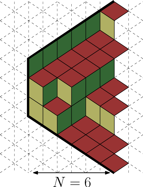
Repeating the bijection we arrive at a correspondence between paths from and lozenge tilings of trapezoids.
Let us fix and consider the set of all paths between and . This is a finite set. Let us equip this set with a uniform probability measure. We are interested in the asymptotic behavior of random paths distributed according to this measure. In terms of lozenge tilings, we consider a uniformly random tiling of a trapezoid of width with prescribed (deterministic) positions of horizontal lozenges along the right boundary.
Repeating (3.16) we now define the (random) height function
of such path. As before, in terms of a lozenge tiling, it
counts the number of horizontal lozenges
![]() above a point . Note
that we now have , as the tiling is not defined outside this range.
above a point . Note
that we now have , as the tiling is not defined outside this range.
As in Section 3.4, the CLT for involves a certain map to the upper half–plane . Let us introduce it.
For a probability measure with compact support on , we define a map , via
Note that the expressions on the right-hand side of the equations above are invariant with respect to complex conjugations, so and are indeed real for any . Let be the image of this map. Also set
Proposition 3.13.
a) Assume that is a probability measure with compact support and density with respect to the Lebesgue measure. Then the map is a diffeomorphism between and .
b) This diffeomorphism can be defined in another way. For fixed consider the equation . Then this equation has either 0 or 1 root in . Moreover, there is a root in if and only if , and if we put into correspondence to the pair the root from we obtain the inverse of the map .
Proof.
As in Section 3.4 we carry the height function over to through
As before, we do not lose any information here, as the tiling is frozen outside and there are no fluctuations, cf. right panel of Figure 2, where the lozenge tiling is frozen outside the circle inscribed into the hexagon.
Define a moment of the random height function as
Also define the corresponding moment of GFF via
Theorem 3.14 (Central Limit Theorem for lozenge tilings).
Suppose that , , is a regular sequence of signatures such that
| (3.18) |
and let be the height function for the uniformly random element of . Then
in the sense that, as , the collection of random variables converges, in the sense of moments, to .
Remark 3.15.
For explicit expressions for the covariance of , see Lemma 9.2.
The proof of Theorem 3.14 is given in Section 9.1, and we believe that in this generality it is new.
The convergence to the Gaussian Free Field for certain lozenge tiling models was first obtained by Kenyon [Ken]. Theorem 3.14 is closely related to the result obtained by Petrov [Pet2]. There are two differences: First, in [Pet2] the convergence is obtained only for measures which consist of finitely many segments with density 1. In Theorem 3.14 an arbitrary measure with compact support is allowed. The second difference is that, though the limit object is the same, the convergence is proved for different sets of observables.
3.6. Domino tilings
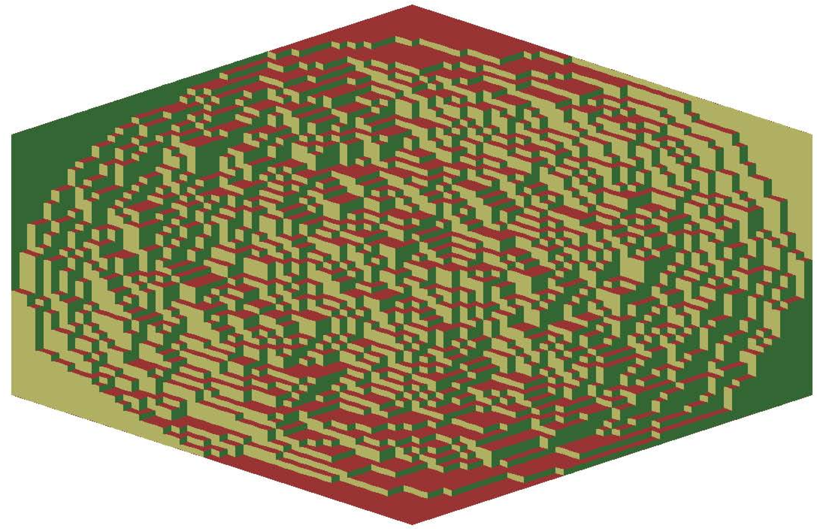
In this section we switch from the triangular grid to the square grid and replace lozenges by dominos. Consider an Aztec diamond of size , which is the side “sawtooth” rhombus drawn on the square grid, as shown in Figure 3. Following [EKLP], we consider tilings of this rhombus with vertical and horizontal dominos. For a positive real it is known that
Let us pick a random tiling of size Aztec diamond according to the probability measure . A sample from this measure for is shown in the right panel of Figure 3.
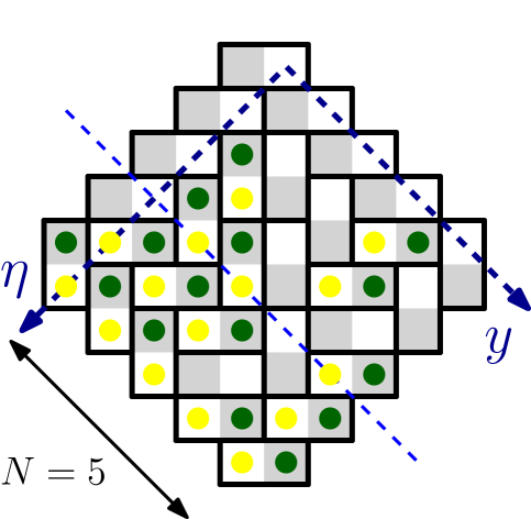
Similarly to Section 3.5, we can identify domino tilings with
sequences of signatures, although the construction is more delicate this time.
Coloring the grid in the checkerboard order, we can distinguish four types of
dominos: two vertical ones
![]() ,
,
![]() and two horizontal
ones
and two horizontal
ones
![]() ,
,
![]() . We further choose
one of the horizontal types and one of the vertical types; for the sake of being
definite let us choose
. We further choose
one of the horizontal types and one of the vertical types; for the sake of being
definite let us choose
![]() and
and
![]() . We stick to these
two types and put green particles on the gray squares (of the checkerboard
coloring) and yellow particles on the white squares, as shown in the left
panel of Figure 3.
. We stick to these
two types and put green particles on the gray squares (of the checkerboard
coloring) and yellow particles on the white squares, as shown in the left
panel of Figure 3.
Reading the yellow particle configuration from up–right to down–left, we observe slices with , , …, particles, respectively; a –particle slice is shown in Figure 3. The particles of the –particle slice have coordinates , which we identify with a signature through
We can now define the height function of uniformly random domino tiling of the size Aztec diamond through the very same formula (3.16) as before. In terms of tilings, the height function counts the yellow particles in the down–right direction on the given diagonal (of fixed and growing ) from the point .
As before we would like to carry the height function to the upper half–plane. For that we need the following proposition.
Proposition 3.16.
For any and the equation
| (3.19) |
has 0 or 1 root in . It has a root in if and only if the pair lies in the ellipse inscribed in the Aztec diamond
The map given by this root is a diffeomorphism. We denote by the inverse of this map.
This proposition coincides with Lemma 5.1 from [CJY].
Let us carry over to — define
For and , define a moment of the random height function as
Also define the corresponding moment of GFF via
Theorem 3.17 (Central Limit Theorem for the domino tilings of the Aztec diamond).
Let be a random function corresponding to the uniformly random domino tiling of the Aztec diamond in the way described above. Then
In more details, as the collection of random variables converges, in the sense of finitely-dimensional distributions, to .
Remark 3.18.
For the explicit expression for the covariance of see (9.16).
3.7. Noncolliding random walks
We proceed to our final application. Here the general framework is to study independent identical random walks on conditioned to have no collisions with each other. This model is quite general, as one can start from different random walks, and also the initial configuration for the conditional process might vary.
Here we stick to three simplest random walks (but it is natural to expect that the results generalize far beyond that). Let be one of the following:
-
•
The continuous time Poisson random walk of intensity .
-
•
The discrete time Bernoulli random walk , where at each moment the particle can either jump to the right by one with probability or stay put with probability .
-
•
The discrete time geometric random walk , where for at each moment the particle jumps to the right steps with probability , .
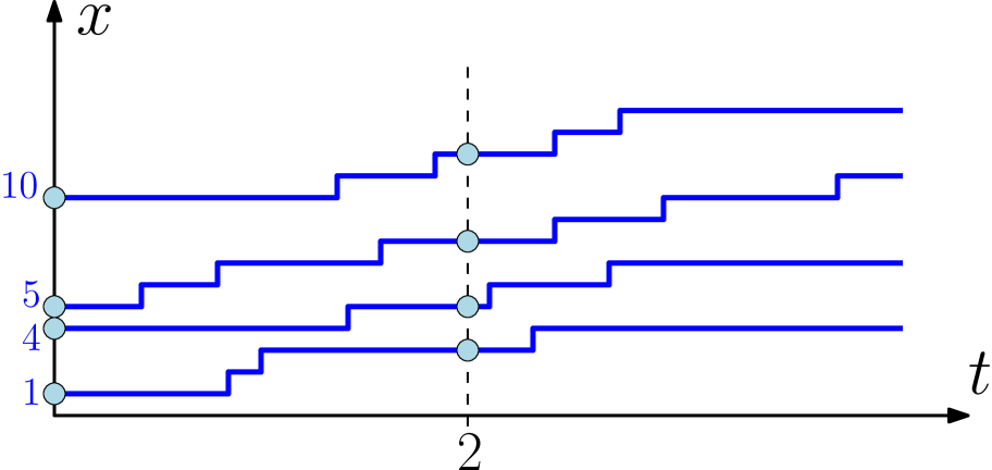
We now define for each the –dimensional noncolliding process . We fix an arbitrary initial condition , take independent identically –distributed random walks started from points ,… and define as the conditional process given that the trajectories of these random walks do not intersect (at all times ), cf. Figure 4. Note that the condition has probability zero, and so one needs to make sense of it. One way here is to start with considering distinct ordered speeds (which correspond to the parameters , or ), and then make them all equal through a limit transition. We refer to [OC], [KOR] for the details of the construction. The result is that is a Markov process, which fits into the formalism of Section 2.3, more specifically, the maps are given by the multiplication, as in Example 2 of Section 2.4.
Let us identify the points of with a signature through
| (3.20) |
In this notation, if and ,… describe at times , then (in the notations of Example 2 in Section 2.4),
| (3.21) |
If , then (this time should be integers)
| (3.22) |
If , then (again are integers)
| (3.23) |
We are in a position to consider the large -limit of these models. For that assume that is given through (3.20) by a signature , and as these signatures are regular in the sense of Definition 3.1. Let us choose some times and consider at . Then using Theorems 8.1, 8.2 for the asymptotic of Schur generating function for , and explicit formulas (3.21), (3.22), (3.23) we can use Theorem 2.10 and obtain the Central Limit Theorem for the global fluctuations of . The fluctuations are asymptotically Gaussian with covariance given by the double contour integral (2.11). It is plausible that the covariance structure can be again described in terms of the Gaussian Free Field, as in Sections 3.4, 3.5, 3.6, but we do not address this question in the present paper.
As far as we know, the CLT for global fluctuations was not addressed before in this generality. The situation is different for a special case of densely packed initial condition . Then for the CLT (and identification with the Gaussian Free Field) was previously addressed in [BF] by the technique of determinantal point processes and in [BBu], [Ku2] by computations in the universal enveloping algebra of . Further, for all three cases (and still ) the CLT for global fluctuations was established in [Dui2] by employing recurrence relations for orthogonal polynomials.
4. Formula for moments
Our method of proof is based on the fact that given the knowledge of Schur generating function of a probability measure, one can compute its moments. In order to do this, one can apply a certain family of differential operators such that the Schur functions are eigenfunctions of these operators. In more details, it is a straightforward computation that for a probability measure on with the Schur generating function we have
More generally, we have
| (4.1) |
and the similar formulas hold for the joint moments of several power sums of coordinates.
Let us address now a general case of Markov chains introduced in Section 2.3. In Proposition 4.3 below we prove a general formula for moments in this setting. Similar formulas for Macdonald processes can be found in [BCGS, Section 4].
We will need the following technical lemmas.
Lemma 4.1.
Assume that the sum
| (4.2) |
absolutely converges in an open neighborhood of the -dimensional torus . Let be a sequence of reals such that , where is a positive real. Then the sum
absolutely converges in an open neighborhood of the -dimensional torus.
Proof.
Let be a real number such that the series (4.2) absolutely converges in . Consider a series
| (4.3) |
where the sum over signs contains terms corresponding to different choices of signs in inside the arguments. Note that this series is convergent. Assume that are positive, and are negative. Then
| (4.4) |
Since for any ’s there is a term of the form (4.4) in the summation (4.3), we obtain that there exists such that the series
is convergent. This implies the statement of the lemma. ∎
Lemma 4.2.
Assume that the series
absolutely converges in an open neighborhood of the -dimensional torus . Let be a sequence of reals such that , where and is a positive real. Then the sum
absolutely converges in an open neighborhood of the -dimensional torus.
Proof.
Set
Then is an analytic symmetric function in a neighborhood of the -dimensional torus. Therefore, is an analytic antisymmetric function and can be written as an absolutely convergent sum of monomials:
Due to antisymmetry we can consider only terms with . Then Lemma 4.1 shows that the sum
is absolutely convergent in some neighborhood of the -dimensional torus. Multiplying this series by the inverse of the Vandermond determinant, we obtain that the desired series
| (4.5) |
absolutely converges in the region for any . Since the series (4.5) consists of analytic functions, the use of the Cauchy integral formula gives the absolute convergence in a neighborhood of the torus. ∎
For a positive integers set
Proposition 4.3.
In notations of Section 2.3 let be positive integers, let , , …, be as in Section 2.3, and let be a probability measure on with the Schur generating function . Assume that is distributed according to (2.3). Then
| (4.6) |
where in the left-hand side we set to 1 all variables after applying all differential operators.
Proof.
We will prove this proposition for ; the proof for general is analogous. We have
Lemma 4.2 shows that this sum is absolutely convergent in an open neighborhood of the -dimensional torus, and, therefore, belongs to .
Thus, one can apply and obtain
Plugging and using (2.3) we obtain the statement of the proposition. ∎
5. Technical lemmas
This section contains the technical ingredients for the proofs of our main theorems.
5.1. Preliminary definitions and lemmas
For any let be a function of variables . For an integer we will say that a sequence of analytic complex functions has an -degree at most if for any (not depending on ) and any indices we have
| (5.1) |
for some constants . In particular, the limit
should exist (this corresponds to ).
Similarly, we will say that a sequence of analytic complex functions has -degree less than if for any (not depending on ) and any indices we have
Our main source of such functions is the following lemma.
Lemma 5.1.
Assume that for , a sequence of functions satisfies the following condition: For any there exists such that
where is an analytic function in the neighborhood of , and the convergence is uniform in the region . Then has a -degree at most . If the function equals 0, then has a -degree less than .
Proof.
Let be indices from (5.1). For computing the expression we can set to 1 all variables such that prior to the differentiation. After this, let us recall that the uniform convergence of complex analytic functions implies
∎
Let have -degree at most , and let have -degree at most . Then it is easy to see that for any index the function has -degree at most , has -degree at most , and has -degree at most .
Lemma 5.2.
Assume that for each , is a symmetric analytic function in an open neighborhood of . Then for any indices the function
| (5.2) |
is analytic in a (possibly smaller) open neighborhood of . If has -degree at most (less than ), then the sequence (5.2) has -degree at most (less than ).
Proof.
[BuG, Lemma 5.4] implies the first claim.
We need to prove that for any indices the limit
| (5.3) |
has the same -degree as the function . Note that we can immediately specialize to all variables except for , . After this, we deal with a statement about the functions with finite (not depending on ) number of variables.
Any coefficient of Taylor expansion of (5.2) can be written as a finite (not depending on ) combination of the Taylor coefficients of the function . Indeed, it was shown in the proof of Lemma 5.4 of [BuG] (see formula (5.4)) that the Taylor coefficient of of the term of -degree from can contribute to the Taylor coefficients of (5.2) of -degree with , where appears because this is the number of variables which were not immediately set to 1.
Therefore, the -degree of (5.3) is at most that of . ∎
Let be a complex analytic function of one variable at the neighborhood of the unity. Let us introduce the notation for the coefficients in its Taylor expansion
Lemma 5.3.
For a function and positive integer we have
Proof.
This is Lemma 5.5 in [BuG]. ∎
Lemma 5.4.
We have
| (5.4) |
Note that we do not set the value of the variable in the left-hand side.
5.2. Expectation-contributing terms
Let us introduce notations which we will use in the rest of Section 5. Let be an appropriate sequence of measures on with the Schur generating function , and limiting functions , , and (see Definition 2.6). In this section we will analyze expressions which eventually contribute to the leading order of the expectation of the moments of the measure .
For an integer let us introduce the notation
| (5.5) |
Lemma 5.5.
The following statements hold:
a) The functions have -degree at most .
b) For any index the functions have -degree at most .
c) For any indices the functions have -degree less than .
Proof.
Since , the function is well-defined in a neighborhood of and we can rewrite (5.5) in the following form:
We will write the result of the application of the differential operator to in the form
| (5.6) |
After the application of all differential operators in (5.5) in this fashion we can cancel in the numerator and the denominator and write as a large sum of factors of the form
| (5.7) |
where are distinct indices, and are nonnegative integers such that and
| (5.8) |
and depends on , but does not depend on or . Since the operator is symmetric, all terms obtained from (5.7) by permuting variables are present in our sums. Therefore, can be represented as a sum
| (5.9) |
where the first sum is subject to (5.8), and we omitted the dependence of on .
Let us now prove three 3 statements of Lemma 5.5.
a) First, let us consider the asymptotics of the expression
Note that each factor has -degree at most , since is an appropriate sequence. Therefore, Lemma 5.2 and equality (5.8) imply that this function has -degree at most. The expression
contains terms of this form; therefore, it has -degree at most .
b) We are interested in the asymptotics of the expression
| (5.10) |
Let us consider two cases.
b1) First, consider a term
| (5.11) |
with . Note that there are such terms. We need to apply the operator to one of the factors , because only these factors depend on in this case. Note that
has -degree at most . Assume that the operator is applied to (other cases can be considered analogously). Then the expression can be written as a sum of terms of the form
Lemma 5.2 asserts that this sum has -degree at most . Recall that . We see that the maximum of -degree is achieved at , , , . It follows that the expression (5.11) has -degree at most . Taking into account that there are terms of such a form, we obtain that the sum has -degree at most .
b2) Now let us consider the term of the form (5.11) with . Since is fixed, there are terms of such form. Note that since the function
has -degree at most , then its derivative also has degree at most . Therefore, the sum of all terms of such a form has -degree at most , which concludes the proof of the claim b).
c) We are interested in the asymptotics of the expression
| (5.12) |
Again, let us consider several cases related to whether indices and are from or not.
c1) If both indices and are outside of , and both differentitations and are applied to same . Since has -degree less than 0, the same considerations as in the case b1) imply the statement of proposition.
c2) If both indices are outside of , and these differentiations are applied to different . It is easy to see that in this case all terms have -degree at most which is even stronger than we need.
c3) If and is outside of this set, then we lose one degree of in the summation over sets of indices and another degree when we differentiate . Therefore, all these terms have -degree at most , what is stronger than we need.
c4) If , then we lose two degrees in the summation over sets of indices. Again, all such terms give contribution -degree at most. This concludes the proof of the lemma. ∎
Remark 5.6.
Note that we have
| (5.13) |
where the function has -degree less than . Indeed, the proof of Lemma 5.5 shows that the highest -degree is obtained in the case , , . A coefficient appears because we need to apply differentiations to and differentiations to .
5.3. Covariance-contributing terms
For positive integers let us define one more function by
| (5.14) |
The meaning of this function is given by the next lemma; essentially, this lemma describes the covariance in our probability models.
Lemma 5.7.
For any positive integers we have
| (5.15) |
where has -degree at most , and has -degree less than .
Proof.
The left-hand side of (5.15) can be written as
Applying differentiations with the use of (5.6), we can rewrite it as the sum of terms of the form
for nonnegative integers , , , such that and
| (5.16) |
From terms with we obtain . Let us deal with other terms.
Let us estimate -degree of all terms with fixed collection of numbers , , . Lemma 5.5 asserts that has -degree at most since . Therefore, the total -degree of these terms is at most (as usual, we apply Lemma 5.2 here). Given (5.16) and , it is clear that this number is maximal for , , , ; for this choice of parameters our sum of terms has -degree at most , and for all other terms the expression is smaller and the total contribution of all other terms have -degree less than .
The terms with , , , are exactly those which are present in the expression (5.14). ∎
Lemma 5.8.
The function has -degree at most . For any index the function has -degree less than .
Proof.
The first statement was proven in the previous lemma. We know that is the sum of terms
over , and all sets . When we differentiate the sum of these terms by , we need to consider two cases. First, the terms with inside has -degree at most , because the index is fixed and the total number of terms has smaller order in . Second, if is outside of , then should be applied to or . By Lemma 5.5 has -degree less than , and our conditions on imply that has -degree less than 1. Therefore, for these terms the -degree also decreases due to this differentiation; we obtain that the total -degree of the expression is less than . ∎
Remark 5.9.
5.4. Product of several moments
For a positive integer and a subset we denote by the set of all pairings of the set . In particular, this set is empty if has odd number of elements. We will also need the notation which stands for the set of all pairings of . For a pairing we denote by the product over all pairs from this pairing.
Proposition 5.10.
For any positive integer and any positive integers we have
| (5.17) |
where has -degree less than .
Proof.
We will prove this statement by induction over . For the statement follows from definition (5.5). For it follows from Lemma 5.7. Assume that we already proved it for . Let us apply the operators , , , and use the induction assumption. We need to analyze the expression
for any choice of the set of indices . Note that an induction hypothesis asserts that has -degree less than . Let us consider several cases to analyze all arising terms.
1) All differentiations are applied to or from . By definition, these terms give rise to the function . The terms obtained in this way have the required form with the set of indices .
2) One differentiation is applied to the function for some , and all other differentiations are applied to . Using Remark 5.9, we see that these terms have the required form with and the arising function in the product of the pairings.
3) Consider all other terms. We will show that they do not contribute to the leading order. We fix the set . Let us define the function
From Lemma 5.8 it follows that has -degree at most , but for any index the function has a -degree less than .
We analyze the expression
As before, we can write the result of the application of our differential operator as a sum of terms of the form
Since has -degree at most , it is easy to see that the highest -degree terms are present in the expression
| (5.18) |
where
| (5.19) |
Let us estimate the -degree of this expression for fixed .
Let be the set of indices such that . Then this term is the product of and a certain symmetric function. Our goal is to show that the -degree of this symmetric function can be estimated as less than , with the exception of cases 1) and 2) considered above, which means that this symmetric function is a part of .
The function has -degree at most . The summation over indices contributes the -degree . If , then has -degree at most . This and (5.19) means that if two different are not equal to 0, then the result has -degree at most . However, if is greater than 0, then we obtain the total -degree less than . Therefore, if the term (5.18) contributes to the degree , then and only one of the indices can be equal to non zero. This leaves out only two possibilities: if all are equal to 0, then we are in the case 1) considered above, and if one of is not equal to 0, then we are in the case 2) considered above. This concludes the proof of the proposition. ∎
5.5. Gaussian behavior
For a positive integer let us set:
| (5.20) |
This is the expectation of the th moment of the probability measure with the Schur generating function .
Lemma 5.11.
For any positive integer and any positive integers we have
| (5.21) |
where has -degree less than .
Proof.
We use (5.17) to compute (5.21), and our goal is to show that the appearance of ’s cancels out all terms from the right-hand side of (5.17) with the non-empty set , and the right-hand side of (5.21) comes from the term with the empty set .
We use the following notation: Let be a subset of ; we denote by the complimentary subset such that . Analogously, for we denote by the complementary subset such that .
Proposition 5.10 yields
| (5.22) |
where
we use an additional superscript here (in comparison with Proposition 5.10) because we apply Proposition 5.10 to a different set of indices. Note that does not depend on the choice of : It depends on only.
Opening the parenthesis in the left-hand side of (5.21), we write it as
| (5.23) |
Applying (5.22) and substituting , we see that (5.23) turns into the sum of terms of the form
| (5.24) |
where , and . The summation goes over all possible choices of and .
Let us fix the set . Note that the same term (5.24) can be obtained for all possible choices of ’s and ’s such that the union of these sets of indices is ; the only difference is the sign . Collecting all terms of this form, we see that the total coefficient is
which is always 0 unless . Therefore, the only term which survives all cancellations in (5.23) is the term with and which in combination with Proposition 5.10 implies Lemma 5.11. ∎
Proposition 5.12.
6. Computation of covariance
6.1. Covariance for extreme characters
In this section we compute the covariance in the setting of Theorem 2.8 for a special class of Schur generating functions (see equation (6.9) below). All computations of this section will be extensively used in the proof of the general result as well.
Let be a complex analytic function in a neighborhood of the unity, and let
| (6.1) |
be the Taylor expansion of at .
Lemma 6.1.
Assume that is a complex number. With the above notations, we have
| (6.2) |
where .
Proof.
The Cauchy integral formula yields
Substituting this into the left-hand side of (6.2) and using the equalities
and
we arrive at the formula
Note that the first term in the right-hand side has no pole inside and, therefore, is equal to 0, while the second term coincides with the right-hand side of (6.2). ∎
Let , be analytic complex functions in a neighborhood of the unity. Let we denote the coefficients determined by (6.1) with . Let us define the functions
| (6.3) |
Lemma 6.2.
With the above notations, we have
| (6.4) |
where the contours of integration are counter-clockwise and .
Proof.
By the Cauchy integral formula we have
Therefore, the left-hand side of (6.4) can be written as
| (6.5) |
The binomial theorem gives
| (6.6) |
Plugging this expression into (6.5) and observing that the term with gives zero contribution (because does not have a pole at zero), we obtain that the left-hand side of (6.4) equals
The definition (6.3) implies that
The binomial theorem and Lemma 6.1 allows to rewrite this expression in the form
We now consider a special case of Theorem 2.8. Let be a sequence of probability measures, where is a probability measure on , and let be reals such that the function
is well defined in a neighborhood of unity. We assume that the Schur generating function has the form
| (6.9) |
where is a sequence of holomorphic functions such that
Clearly, such a Schur generating function is appropriate in the sense of Section 2.2 with , , and .
Proposition 6.3.
Proof.
We denote by the equality of highest -degree.
As explained in Section 4, we have
| (6.10) |
Therefore, Lemma 5.7 implies that
| (6.11) |
Let us compute the right-hand side of this formula. By definition (5.14),
| (6.12) |
The right-hand side of the approximate equality in (6.12) contains only leading terms from , see (5.13); it is proven by following the same arguments as in Section 5.2.
Now we will use the special form (6.9) of our function . In this case we see that . Therefore,
| (6.13) |
Let us analyze this expression for different ’s and ’s. Note that we must have in order to get a non-zero contribution. Also we see that if , then the total -degree is not greater than ( and come from the power of , , , and come from the summation over sets of indices); therefore, these terms do not contribute to the -degree . We obtain that only terms with contribute to the limit.
For these terms we use Lemma 5.4 for the symmetrization over ’s and obtain:
| (6.14) |
where we use the notation (6.3) with . We also use that the summation contains terms. For the symmetrization over ’s it is enough to apply Lemma 5.3. We obtain
| (6.15) |
Thus,
Now Lemma 6.2 with and implies the statement of the proposition. ∎
6.2. Computation of one-level covariance in the general case
Here we compute the covariance in Theorem 2.8. We use computations and arguments from the special case considered in the previous section.
Proposition 6.4.
Let be an appropriate sequence of measures on , , and corresponding to functions and . In notations of Theorem 2.8 we have
Proof.
For an integer we denote by any function of variables which has -degree less than , and which can change from line to line.
We start our analysis with formulas (6.11) and (6.12) for covariance. Let us fix indices and , and consider several cases.
1) Assume that . Then
Note that the definition of an appropriate sequence of Schur generating functions implies that has -degree at most , and has -degree at most . Moreover, we have
| (6.16) |
Using these equalities and Lemma 5.2, we get
| (6.17) |
Note that the first term in the right-hand side of (6.17) depends on variables, not on variables. The dependence on all variables is present only in ; our notion of -degree and Lemma 5.2 guarantee that eventually this function does not contribute to the covariance.
Using (6.16), (6.17) and Lemma 5.2 again, we further obtain
| (6.18) |
The summation over non-intersecting sets and in (6.12) contributes the terms. Applying Lemma 5.3 to (6.18) and using equality , we see that the case of non-intersecting indices contributes the term
| (6.19) |
into the leading order. With the use of the Cauchy integral formula and the binomial theorem ( which is applied in the same way as in (6.6)) one can write it in the form
| (6.20) |
2) Assume that . Without loss of generality we can assume that , and all other indices are distinct. Similarly to the case 1), one can use equality (6.16) to show that
| (6.21) |
Note that the summation over indices produces order terms in this case in (6.12), so the function does not contribute to -degree . The first term in the right-hand side of (6.21) gives rise to exactly the same computation as in Proposition 6.3. As we proved in Proposition 6.3, the contribution of this term to -degree can be written as
| (6.22) |
It is interesting to note that while this term has very similar form to (6.20), we obtain it as a result of rather lengthy computations of the whole Section 6.1, though the computation behind (6.20) in case 1) is much simpler.
3) Assume that . Then the same argument as in case 2) shows that for the fixed indices the function in the left-hand side of (6.21) has a -degree not greater than , while the summation over all such indices contributes only . Therefore, all such terms do not contribute to .
It remains to conclude that the contribution to the -degree is given by the sum of expression from (6.20) and (6.22). Therefore, recalling the definition of given in Definition 2.6, we are done.
∎
6.3. Covariance in Theorems 2.9, 2.10, 2.11
The arguments of Section 6.2 need only minor modifications in order to compute the covariance in Theorems 2.9, 2.10, 2.11. In each case, we start with a general formula for moments (4.6) and analyze it in the same way as in the case of one level.
Covariance in Theorem 2.9.
In this case the joint moments on different levels are given by the following differential operators
The only difference with computations in Sections 6.1 and 6.2 is that in (6.12) the set is the subset of and the set is the subset of . This leads to the appearance of the factor inside of summations in (6.19) and (6.15). The arising modification of computations is given by Lemmas 6.1 and 6.2 with and . This gives rise to two functions
instead of one function (as before, we identify the function from Section 6.1 and ). In the end, we obtain
Covariance in Theorem 2.10.
In this case the moments of power sums are given by the following differential operators
Therefore, the right-hand side of (6.12) has a form
| (6.23) |
(recall that the functions are defined in (2.10)).
The analysis of this expression goes in exactly the same way as before. The only difference is that instead of (6.16) we need to plug
into (6.23). The appearance of two different functions and instead of one function leads to a modification of computations of Section 6.2 which is covered by Lemmas 6.1 and 6.2 with and . This gives the covariance in Theorem 2.10.
Covariance in Theorem 2.11
The moments of power sums are given by
The analysis goes in the same way as in the previous two cases with both changes made simultaneously.
7. Asymptotic normality
7.1. Gaussianity: Theorem 2.8
In the notations of Theorem 2.8 we prove the asymptotic normality of the vector .
Note that for any we have For any in Section 6.2 we showed that the quantity
exists (and also computed it).
Proposition 7.1.
For any positive integers we have
if is odd, and
where is the set of all pairings of .
Proof.
One sees that
Therefore, the statement of the proposition is a direct corollary of Proposition 5.12. ∎
7.2. Gaussianity: Theorems 2.9, 2.10, 2.11
We denote by the set of variables .
We use a general formula (4.6) for moments. In the notations of Theorem 2.11, for arbitrary and , , we have
The analysis of this formula is exactly the same as in Sections 5.4, 5.5, and 7.1. Let us indicate necessary modifications of notations. For instead of (5.5) we consider the function
| (7.1) |
For instead of (5.14) we use the function
| (7.2) |
Instead of (5.20) we use . With these changes, all the analysis of Sections 5 and 7.1 goes in exactly the same way, which gives us the asymptotic normality of functions .
8. Asymptotics of Schur functions
In this section we recall and extend certain asymptotics of normalised Schur functions, which were developed in [GM], [GP], [BuG].
Recall that we encode a signature by a discrete probability measure on via
We use the notation from Section 3.1. The following theorem is a special case of Theorem 4.2 from [BuG].
Theorem 8.1 ([GM],[GP], [BuG] ).
Suppose that , is a regular sequence of signatures (see Definition 3.1 ), such that
Then for any we have
| (8.1) |
where the convergence is uniform over an open complex neighborhood of .
Theorem 8.2.
Suppose that , is a regular sequence of signatures such that
Then we have
| (8.2) |
and
where the convergence is uniform over an open complex neighborhood of .
Remark 8.3.
Note that the limit in (8.2) does not depend on .
Proof of Theorem 8.2.
Let us consider the application of the differential operator . Each differentiation from it can be applied to for some or to the factors appeared from the other differentiations. Note that the highest degree in is obtained when each differentiation is applied to . Using Theorem 8.1 we obtain
(here and below the convergence in is uniform over an open complex neighborhood of ). Hence,
where we use that the uniform convergence of analytic functions implies the convergence of its derivatives. Substituting this formula into (8.3), we get
Also we see that
Recall that for a representation of we define a probability measure on with the use of (3.6). The pushforward of with respect to the map is a random probability measure on that we denote .
Proposition 8.4.
Assume that , , are two regular sequences of signatures such that
for probability measures and with compact supports. Then is an appropriate probability measure on with functions
9. Proofs of applications
9.1. Lozenge tilings and Gaussian Free Field
In this section we prove Theorem 3.14.
Recall that we study the uniform measure on the set of paths . The projection of this measure to one level , , produces a probability measure on . The branching rule for Schur functions (2.4) shows that its Schur generating function equals .
For , let be moments of these measures:
Note that they are random variables.
Proposition 9.1.
Proof.
Proposition 9.1 shows that the fluctuations in our model are Gaussian. We next recover the structure of the Gaussian Free Field, for that we transform the expression for the covariance.
Lemma 9.2.
Proof.
Let us make a change of variables in (9.2)
this change of variables is well-defined since we are dealing with analytic functions in a neighborhood of the origin.
Using the relation between and (see equation (3.5)), we have
Substituting these equalities, we obtain that (9.2) equals
Making a further change of variables , , we arrive at (9.4).
∎
Proof of Theorem 3.14 .
We recall that the functions and were defined in Section 3.5.
For let be the union of the set and its conjugate. A direct check shows that if then . Therefore, for the contour contains the contour . Thus, in (9.4) we can deform the contour to and the contour to without meeting poles of the integrand. We obtain
| (9.5) |
Recall that the values of are real. Using this fact and the equality
we can rewrite this expression as
| (9.6) |
(in this equation we are integrating over curves in the upper half-plane only).
Let us now transform the quantities involved in the statement of the theorem. An integration by parts gives us
Therefore, Proposition 9.1, Lemma 9.2 and equations (9.5), (9.6) show that the collection converges to the Gaussian limit and the limit covariance is given by
The definition of the Gaussian Free Field implies
An integration by parts shows that the right-hand sides of two equations differ by a factor . This concludes the proof of the theorem. ∎
9.2. Extreme characters of and Gaussian Free Field
Recall that is a Stieltjes transform of measure on the real line (see (3.3)).
Lemma 9.3.
Assume that a sequence of extreme characters satisfies the condition (3.14) with the limiting sextuple . Then we have the convergence
where is given by the formula
| (9.7) |
Proof.
The explicit formula for comes as a direct computation from the Voiculescu formula (3.12). ∎
We will need the following elementary technical statement about the measures on ; we omit its proof.
Lemma 9.4.
For each finite measure on with compact support there exists a sequence of measures such that
and has a density with respect to Lebesgue measure which does not exceed .
For a measure and let be a shift of into , that is
For a measure and we denote by the measure
For a set let be a set obtained from by reflecting with respect to . For a measure we denote by the measure
We denote by the union (equivalently, the sum )of measures and .
Lemma 9.5.
Assume that is a sextuple that appears in the limit in the condition (3.14). Then there exists a sequence of probability measures with bounded by densities with respect to the Lebesgue measure on such that theirs Stieltjes’ transforms satisfy:
| (9.8) |
as .
Proof.
First, note that is the Stieltjes transform of the uniform measure on . Next, we will consider several other signed measures with total weight which give rise to other terms in expression (9.8). It follows that the union of the uniform measure on and all signed measures will have weight , and we will check that it is a probability measure.
Let be a (negative) measure with the density on the segment . Let (note that the total weight of is ). Then the measure has total zero weight and the Stieltjes transform of the form .
Let be a (positive) measure with the density on the segment . Let be a sequence of measures given by Lemma 9.4 applied to the measure . Then the measure has total zero weight and the Stieltjes transform of the form .
The measures for and are constructed in an analogous way. In order to obtain the term let us consider the measure which has density on the interval and density on the interval . In an analogous way we obtain the term .
Finally, let us notice that all negative measures in the construction above are placed on the segment from to (recall that beta parameters are bounded by , see (3.12) ) and has densities which decrease with . In the same time, all positive parts in the constructed signed measures lie outside of the segment . Therefore, for large the union of all these 6 measures with total weight zero and the uniform measure (with weight ) on the segment forms a probability measure which has a required form of the Stieltjes transform, and the density of this measure does not exceed . ∎
Proof of Proposition 3.9.
We prove this Proposition by a limit transition from Proposition 3.13.
Let be a large real number. Let us consider the probability measure on which is given by Lemma 9.5. Let us apply Proposition 3.13 to the measure . As a result, we obtain a diffeomorphism between and . For a fixed pair it is given by a unique root of the equation
| (9.9) |
which lies in (the uniqueness of such a root is a part of Proposition 3.13). We can rewrite it in the form
Let us now set , , for some fixed and . For large we obtain
| (9.10) |
Note that Lemma 9.3 and Lemma 9.5 show that
| (9.11) |
Plugging (9.11) into (9.10), cancelling and multiplying by , we get
| (9.12) |
Let us do a change of variables . Equation (9.12) shows that
| (9.13) |
which has a form given by Proposition 3.9.
Note that the function
is analytic and converges uniformly on compact sets inside as . Therefore, the number of zeros of this function inside cannot increase in the limit as . Thus, for any pair the equation (9.13) has no more than one solution in , which shows the existence of from the statement of Proposition 3.9 and the existence of the map .
On the other side, the bijection is given by the explicit formulas:
( these functions are solutions to (9.9) ). In the limit and with the change of variables as above, these functions converge to the functions
Note that for any these limiting functions are solutions to (9.13) with and . Therefore, the map is a bijection. Moreover, this is a diffeomorphism since the functions and are differentiable, and the differentiability of the map is provided by the Implicit Function theorem.
Proof of Theorem 3.10.
Recall that we have a probability measure on the set of paths in the Gelfand-Tsetlin graph. Let be the shifted moments of the random signature distributed according to this measure:
Our probabilistic model clearly satisfies assumptions of Theorem 2.9, with , and . Applying it, we obtain that the random variables converge to the jointly Gaussian limit with zero mean and covariance
| (9.14) |
where and .
Note that the formula (9.14) for covariance already contains the cross factor — this is a key indication of the presence of the Gaussian Free Field. The derivation of Theorem 3.10 from (9.14) is completely analogous to the derivation of Theorem 3.14 from (9.4) modulo the fact that one needs to use Proposition 3.9 instead of Proposition 3.13 in order to deal with the arising level curves. ∎
9.3. Domino tilings of Aztec diamond and Gaussian Free Field
In this section we prove Theorem 3.17.
Let us formally describe the probability measure on a particle system which turns out to be equivalent to the domino tiling model.
For each let , be signatures of length , and let , where is a parameter from Section 3.6.
Define the coefficients via
Recall that the coefficients were defined in Section 2.4. The branching rule and the Pieri rule for Schur polynomials imply that the coefficients and are nonnegative.
Define the probability measure on the sets of signatures of the form by the formula
| (9.15) |
(it can be directly checked by induction that the total sum of these weights is 1). Let be the set of such configurations that has a nonzero probability measure.
Proposition 9.6.
There is a bijection between and the set of domino tilings of the Aztec diamond of size . Moreover, under this bijection the measure (9.15) turns into the measure on the set of domino tilings of the Aztec diamond of size .
Proof.
This fact is well-known, and essentially two sequences of signatures are yellow and green particles in Figure 3. It was implicitly used in [J2] and [BorFe]; for a recent exposition, see [BCC]. See also [BuK], where a generalization of this construction is used for a study of domino tilings of more general domains. ∎
The bijection described in Proposition 9.6 allows to translate all results about a two-dimensional particle array into the geometric language of domino tilings. We will now proceed in the language of arrays.
Proof of Theorem 3.17.
Let be random signatures distributed according to the measure (9.15). For let be the -th power degree of the coordinates of the signature . That is, we have
Proposition 9.7.
In the notations of Theorem 3.17, the collection of random variables is asymptotically Gaussian with the limit covariance
| (9.16) |
where and .
Proof.
Notice that the equation (9.16) contains the cross factor . Using , one directly checks that the equation
coincides with the equation given in Proposition 3.16. Theorem 3.17 can be obtained from Proposition (9.7) with the use of Proposition 3.16 in exactly the same way as in the previous two sections. ∎
9.4. Tensor products and degeneration to random matrices
There exists a way to degenerate the tensor products of representations into sums of Hermitian matrices, see e.g. Section 1.3 of [BuG] for details. Our goal is to show that under this degeneration the covariance for tensor products (given in Theorem 3.3) turns into the covariance for the sum of random matrices.
Let and , , be two sets of reals, let be a diagonal matrix with eigenvalues , and let be a diagonal matrix with eigenvalues . Assume that is a uniformly (=Haar-distributed) random unitary matrix. Let
and let be (random) eigenvalues of . Set
Assume that
where are probability measures on with compact supports.
Let
where by we mean the functional inverse of the function , and the function was introduced in Section 3.1.
In the limit regime the covariance of the functions is given by the following formula, see [PS, Chapter 10]
where the contours encircle infinity and no other poles of the integrand.
Let us make a change of variables (i.e. ), which, in particular, swaps with . Note that conveniently is a differential form for an arbitrary function , and thus it does not change at all. Therefore, we obtain
| (9.17) |
where contours of integration encircle zero and no other poles.
Recall the setting and notations of Theorem 3.3. Let be two limiting measures for signatures. Theorem 3.3 asserts that random variables which corresponds to the measure have the covariance given by the formula
| (9.18) |
where contours of integration encircle zero and no other poles.
Proposition 9.8.
10. Appendix: Law of Large Numbers
In this section we prove Theorem 2.4. In fact, this is [BuG, Theorem 5.1], and we comment on slight differences here.
The first difference is that [BuG, Theorem 5.1] requires that the Schur generating function of a probability measure satisfies the condition
where is a holomorphic function and the convergence is uniform in an open neighborhood of . It is clear that this condition implies the properties of Definition 2.1 with , for . The uniform convergence of holomorphic functions implies the convergence of Taylor coefficients, though the opposite is not always correct. However, in the proof of Theorem 5.1 from [BuG] we use only the convergence of Taylor coefficients, so the same proof (see Section 5.2 of [BuG] ) goes without any changes.
References
- [AGZ] G. W. Anderson, A. Guionnet, O. Zeitouni, An Introduction to Random Matrices, Cambridge University Press, 2010.
- [Bi] P. Biane, Approximate factorization and concentration for characters of symmetric groups, International Mathematics Research Notices 2001 (2001), no. 4, 179–192.
- [BCGS] A. Borodin, I. Corwin, V. Gorin, S. Shakirov, Observables of Macdonald processes, Transactions of the American Mathematical Society, 368 no.3, pp 1517-1558, (2016), arXiv:1306.0659.
- [BorFe] A. Borodin, P. Ferrari. Anisotropic growth of random surfaces in 2 + 1 dimensions, Communications in Mathematical Physics, nol. 325, no. 2, pp 603-684, (2014) arXiv:0804.3035.
- [BO] A. Borodin, G. Olshanski. The boundary of the Gelfand-Tsetlin graph: a new approach, Advances in Math. 230 (2012), 1738–1779, arXiv:1109.1412.
- [BBu] A. Borodin, A. Bufetov, Plancherel representations of and correlated Gaussian Free Fields, Duke Math. J. 163, no. 11 (2014), 2109-2158, arXiv:1301.0511.
- [BBO] A. Borodin, A. Bufetov, G. Olshanski. Limit shapes for growing extreme characters of U(infty), Annals of Applied Probability, Vol. 25, no. 4, (2015), 2339-2381, arXiv:1311.5697.
- [BC] A. Borodin, I. Corwin, Macdonald Processes, Probability Theory and Related Fields, 158, no. 1-2 (2014), 225–400. arXiv:1111.4408.
- [BF] A. Borodin, P. Ferrari, Anisotropic Growth of Random Surfaces in 2 + 1 Dimensions, Communications in Mathematical Physics, 325, no. 2, (2014) 603–684. arXiv:0804.3035.
- [BGG] A. Borodin, V. Gorin, A. Guionnet, Gaussian asymptotics of discrete –ensembles, Publications mathématiques de l’IHÉS 125, no. 1 (2017), 1–78, arXiv:1505.03760.
- [BCC] J. Bouttier, G. Chapuy, S. Corteel. From Aztec diamonds to pyramids: steep tilings,Trans. Amer. Math. Soc. 369 (2017), 5921–5959, arXiv:1407.0665.
- [BrDu] J. Breuer, M. Duits, Central Limit Theorems for Biorthogonal Ensembles and Asymptotics of Recurrence Coefficients, to appear in Journal of American Mathematical Society, arXiv:1309.6224.
- [BuG] A. Bufetov, V. Gorin. Representations of classical Lie groups and quantized free convolution, Geom. Funct. Anal., Vol. 25 (2015) 763-814, arXiv:1311.5780.
- [BuG2] A. Bufetov, V. Gorin, Fourier transform on high–dimensional unitary groups with applications to random tilings. Duke Mathematical Journal, 168, no. 13 (2019), 2559–2649, arXiv:1712.09925.
- [BuK] A. Bufetov, A. Knizel. Asymptotics of random domino tilings of rectangular Aztec diamonds, Ann. Inst. H. Poincaré Probab. Statist. 54, no. 3 (2018), 1250–1290, arXiv:1604.01491
- [C] P. Cartier. Introduction a l’etude des mouvements browniens a plusieurs parametres, Seminaire de probabilites (Strasbourg), 5:58–75, 1971.
- [CJY] S. Chhita, K. Johansson, B. Young, Asymptotic domino statistics in the Aztec diamond, Annals of Applied Probability, 25, no. 3 (2015), 1232–1278. arXiv:1212.5414.
- [DF] M. Dolega and V. Feray, Gaussian fluctuations of Young diagrams and structure constants of Jack characters, Duke Mathematical Journal, 165, no. 7 (2016), 1193–1282, arXiv:1402.4615.
- [Dub] J. Dubedat, SLE and the free field: Partition functions and couplings, Journal of the American Mathematical Society, 22, no. 4 (2009), 995–1054, arXiv:0712.3018.
- [Dui1] M. Duits, The Gaussian free field in an interlacing particle system with two jump rates, Communications on Pure and Applied Mathematics, 66 , no. 4 (2013), 600–643. arXiv:1105.4656
- [Dui2] M. Duits, On global fluctuations for non-colliding processes, Annals of Probability, 46, no. 3 (2018), 1279–1350, arXiv:1510.08248.
- [Dur] R. Durrett, Probability: theory and examples, Forth edition, Cambridge University Press, 2010.
- [DM] E. Duse, A. Metcalfe. Asymptotic geometry of discrete interlaced patterns: Part I, Int. J. Math. 26, 1550093 (2015), arXiv:1412.6653.
- [E] A. Edrei. On the generating function of a doubly infinite, totally positive sequence, Trans. Amer. Math. Soc. 74:367–383, 1953.
- [EKLP] N. Elkies, G. Kuperberg, M. Larsen, J. Propp, Alternating-sign matrices and domino tilings, J. Algebraic Combin. 1 (1992), no. 2, 111–132; no. 3, 219-234. arXiv:math/9201305.
- [F] J. Fulman, Stein’s method, Jack measure, and the Metropolis algorithm, Journal of Combinatorial Theory, Series A, 108, no. 2 (2004), 275–296, arXiv:math/0311290.
- [FH] W. Fulton, J. Harris, Representation Theory: A First Course, Springer–Verlag, New York, 1991.
- [GP] V. Gorin, G. Panova, Asymptotics of symmetric polynomials with applications to statistical mechanics and representation theory, Annals of Probability, Vol. 43, No. 6 (2015), 3052-3132, arXiv:1301.0634.
- [GM] A. Guionnet, M. Maïda, A Fourier view on the R-transform and related asymptotics of spherical integrals, Journal of Functional Analysis, 222 (2005), no. 2, 435–490. arXiv:math/0406121.
- [HO] A. Hora and N. Obata, Quantum probability and spectral analysis on graphs, Springer Science & Business Media, 2007.
- [HMP] X. Hu, J. Miller and Y. Peres, Thick points of the Gaussian free field, Annals of Probability 2010, 38, no. 2, 896–926, arXiv:0902.3842.
- [IO] V. Ivanov and G.‘Olshanski, Kerov’s central limit theorem for the Plancherel measure on Young diagrams. In: S.Fomin, editor. Symmetric Functions 2001: Surveys of Developments and Perspectives (NATO Science Series II. Mathematics, Physics and Chemistry. Vol.74), Kluwer, 2002, pp. 93-151, arXiv:math/0304010.
- [J1] K. Johansson, On fluctuations of eigenvalues of random Hermitian matrices, Duke Mathematical Journal, 91 (1998), 151–204.
- [J2] K. Johansson, Non-intersecting Paths, Random Tilings and Random Matrices, Probability Theory and Related Fields, vol. 123, no. 2, (2004), 225-280. arXiv:math/0011250.
- [JN] K. Johansson, E. Nordenstam, Eigenvalues of GUE minors, Electronic Journal of Probability 11 (2006), paper 50, 1342-1371. arXiv:math/0606760.
- [Ka] O. Kallenberg, Foundations of modern probability, Second edition. Springer, 2001.
- [Ker] S. Kerov, Gaussian limit for the Plancherel measure of the symmetric group, Comptes Rendus Acad. Sci. Paris, Serie I, 316 (1993), 303–308
- [Ken] R. Kenyon, Height fluctuations in the honeycomb dimer model, Comm. Math. Phys., 281, (2008), 675-709, arXiv:math-ph/0405052.
- [KOR] W. König, N. O’Connell, and S. Roch. Non-colliding random walks, tandem queues, and discrete orthogonal polynomial ensembles. Electron. J. Probab, 7(5):1-24, 2002.
- [Ku1] J. Kuan, The Gaussian free field in interlacing particle systems, Electronic Journal of Probability, 19 , no. 72 (2014), 1–31, arXiv:1109.4444.
- [Ku2] J. Kuan, Three-dimensional Gaussian fluctuations of non-commutative random surfaces along time-like paths, to appear in Advances in Mathematics, arXiv:1401.5834.
- [Ma] I. G. Macdonald, Symmetric functions and Hall polynomials, Second Edition. Oxford University Press, 1999.
- [MN] S. Matsumoto, J. Novak, A Moment Method for Invariant Ensembles, in preparation.
- [Mel] P.L. Méliot. Kerov’s central limit theorem for Schur-Weyl measures of parameter 1/2, Preprint, 2010, arXiv:1009.4034.
- [MS] J. A. Mingo, R. Speicher, Second Order Freeness and Fluctuations of Random Matrices: I. Gaussian and Wishart matrices and Cyclic Fock spaces, J. Funct. Anal. 235 (2006), no. 1, 226–270, arXiv:math/0405191.
- [MSS] J. A. Mingo, P. Sniady, R. Speicher, Second Order Freeness and Fluctuations of Random Matrices: II. Unitary Random Matrices, Advances in Mathematics, 209, no. 1, (2007), 212–240, arXiv:math/0405258.
- [Mo] A. Moll, Random Partitions and the Quantum Benjamin-Ono Hierarchy, preprint, arXiv:1508.03063.
- [NS] A. Nica and R. Speicher, Lectures on the Combinatorics of Free Probability, Cambridge University Press, 2006.
- [No] J. Novak, Lozenge tilings and Hurwitz numbers, Journal of Statistical Physics, 161, no. 2 (2015), 509–517, arXiv:1407.7578.
- [OC] N. O’Connell, Conditioned random walks and the RSK correspondence, J. Phys. A: Math. Gen. 36 (2003) 3049–3066
- [OO] A. Okounkov, G. Olshanski. Asymptotics of Jack polynomials as the number of variables goes to infinity, Inter. Math. Res. Notices 1998(13):641–682, arXiv:q-alg/9709011.
- [OR] A. Yu. Okounkov, N. Yu. Reshetikhin, The birth of a random matrix, Moscow Mathematical Journal, 6, no. 3 (2006), 553–566.
- [Pan] G. Panova, Lozenge Tilings with Free Boundaries, Letters in Mathematical Physics, November 2015, Vol. 105, Issue 11, 1551-1586, arXiv:1408.0417.
- [PS] L. Pastur, M. Shcherbina. Eigenvalue Distribution of Large Random Matrices, American Mathematical Society, 2011.
- [Pet2] L. Petrov, Asymptotics of Uniformly Random Lozenge Tilings of Polygons. Gaussian Free Field, Annals of Probability, 43 (2014), no. 1, 1–43, arXiv:1206.5123.
- [Sh] S. Sheffield. Gaussian free fields for mathematicians, Probability Theory and Related Fields, 139:521–541, 2007, arXiv:math/0312099.
- [VK] A. M. Vershik, S. V. Kerov. Characters and factor representations of the infinite unitary group. Doklady AN SSSR 267(2):272–276, 1982 (Russian); English translation: Soviet Math. Doklady 26:570–574, 1982.
- [Vo] D. Voiculescu. Representations factorielles de type de , J. Math. Pures et Appl. 55:1–20, 1976.
- [VDN] D. Voiculescu, K. Dykema, and A. Nica, Free random variables, CRM Monograph Series, vol. 1, American Mathematical Society, Providence, RI, 1992.
- [W] H. Weyl, The Classical Groups: Their Invariants and Representations. Princeton, University Press, 1939.
- [Zh] D. P. Zhelobenko, Compact Lie groups and their representations, Translations of Mathematical Monographs, v. 40, AMS, 1978.
- [Z] J. Zinn-Justin, Path integrals in quantum mechanics, Oxford University Press, 2005.