Fluid-poroviscoelastic structure interaction problem with nonlinear geometric coupling
Abstract
We investigate weak solutions to a fluid-structure interaction (FSI) problem between the flow of an incompressible, viscous fluid modeled by the Navier-Stokes equations, and a poroviscoelastic medium modeled by the Biot equations. These systems are coupled nonlinearly across an interface with mass and elastic energy, modeled by a reticular plate equation, which is transparent to fluid flow. We provide a constructive proof of the existence of a weak solution to a regularized problem. Next, a weak-classical consistency result is obtained, showing that the weak solution to the regularized problem converges, as the regularization parameter approaches zero, to a classical solution to the original problem, when such a classical solution exists. While the assumptions in the first step only require the Biot medium to be poroelastic, the second step requires additional regularity, namely, that the Biot medium is poroviscoelastic. This is the first weak solution existence result for an FSI problem with nonlinear coupling involving a Biot model for poro(visco)elastic media.
1 Introduction and motivation
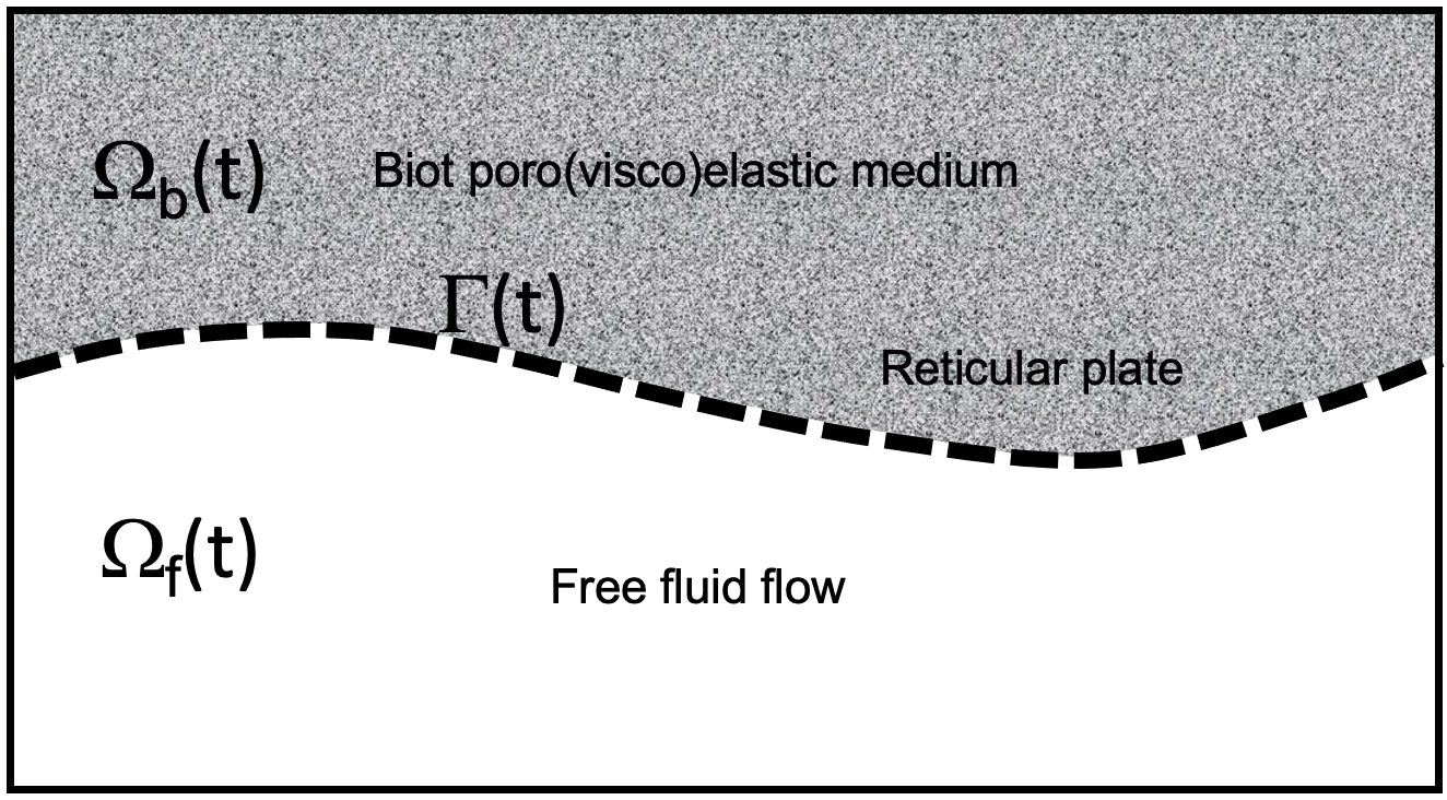
In this paper we study a time-dependent nonlinearly coupled fluid-structure interaction problem between the flow of an incompressible, viscous fluid, modeled by the Navier-Stokes equations, and bulk poroviscoelasticity modeled by the Biot equations. Bulk poroviscoelasticity means that the dimensions of the “free fluid flow” domain and the poroviscoelastic medium domain are the same. In particular, in this manuscript we consider a 2D fluid-poroelastic structure interaction (FPSI) problem, which captures the main mathematical difficulties of such coupling, see Fig. 1. The free fluid flow and the Biot poro(visco)elastic medium are coupled across the current location of the interface, which is modeled by a reticular plate that has inertia and elastic energy. A reticular plate is a lattice-type structure characterized by two properties: periodicity and small thickness, where periodicity refers to periodic cells (holes) distributed in all directions [26]. The reticular plate interface is transparent to fluid flow. We are interested in the existence of finite energy weak solutions (of the Leray-Hopf type).
The problem we study here arises in many applications. In particular, we mention encapsulation of bioartificial organs [70] and blood flow in arteries which are modeled as poro(visco)elastic media to study drug transport through the vascular walls [18, 17, 3]. The reticular plate can be used to capture the elastodynamics behavior of the intima/elastic laminae layer of arterial walls which is in direct contact with the blood flow on one side, and a poroelastic medium consisting of the arterial media/adventitia complex on the other side.
From the mathematical point of view the primary difficulties in studying Navier-Stokes equations nonlinearly coupled to bulk poro(visco)elasticity arise from the fact that the finite energy solutions do not posses sufficient regularity to (1) define the moving domain and the corresponding traces, and (2) guarantee that all the integrals in the weak formulation of the problem are well-defined. The first issue is related to the difficulties associated with fluid-structure coupling, where the fluid and structure domains are of the same dimension. The second issue is a consequence of the geometric nonlinearities associated with moving domain problems. These are the main reasons why to this day there have been no works on the existence of weak solutions for the Biot-Navier-Stokes coupled problems in which the coupling is assumed over a moving interface.
To get around these difficulties, we take the following approaches. First, the reticular plate at the interface associates mass and elastic energy to the interface, and regularizes the boundary of the fluid domain. In classical fluid-structure interaction problems involving elastic structures, this usually takes care of the issues related to the regularity of traces in moving boundary problems [58]. In the case when the structure is poroelastic, and it satisfies the Biot equations on a moving domain, this is, however, not sufficient since the energy estimates do not provide sufficient regularity of the poroelastic matrix displacement for certain integrals over the moving Biot domain in the weak formulation to be well defined. This is why we take the following two-step approach:
-
1.
We introduce a “consistent regularized weak formulation” of the coupled problem by defining a suitable convolution in spatial variables and regularizing only the problematic terms in the weak formulation of the coupled problem. We prove the existence of a weak solution to this regularized problem.
-
2.
We show that as the regularization parameter tends to zero, the solution to this regularized problem converges to the solution of the original nonregularized problem in the case when the original problem has a classical solution and the Biot poroelastic matrix is viscoelastic. Here, a classical solution is a solution that is smooth both temporally and spatially and it hence satisfies the system of PDEs for the original fluid-poroelastic structure problem pointwise.
The existence of a weak solution to the regularized problem was announced by the authors in [44], where only the main steps of the proof were outlined. In particular, the proofs of the existence of weak solutions to the fluid and structure subproblems used in constructing the coupled solution were omitted in [44], and only the main steps of the uniform estimates were presented. Most importantly, the proof of the main compactness result needed to address the main difficulty, the geometric nonlinearity in the regularized problem, is only outlined in [44]. Furthermore, details of the construction of appropriate test functions that are defined on moving domains are also omitted in [44]. Here we present details of all proofs, and show the weak-classical consistency result outlined in step 2 above.
The weak-classical consistency result outlined in step 2 is obtained by using a Gronwall-type estimate, which shows that the energy of the difference between the weak solution of the regularized problem and the classical (temporally and spatially smooth) solution to the original, nonregularized problem with viscoelastic Biot poroelastic matrix, converges to zero as the regularization parameter tends to zero. While the main idea is simple, the estimates are quite nontrivial due to the fact that we need to work with the integrals over regularized Biot domains and compare them with the integrals over the nonregularized moving domains. Details are presented in Section 10.
We conclude this section by noting that the main steps of the constructive proof presented in this manuscript can be used to design a numerical scheme to capture the solutions to the original (non-regularized) FPSI problem, see [62]. The main constructive steps of the proof can be summarized as follows. We semidiscretize the regularized FPSI problem in time by subdividing the time interval into subintervals of width . At each time step we split the reticular plate subproblem from the regularized fluid-Biot subproblem using a Lie operator splitting strategy [35]. To deal with the moving domains we use the Lagrangian map for the Biot domain, and an Arbitrary Lagrangian-Eulerian mapping for the fluid domain, which maps a fixed, reference domain onto the current, physical domain. We switch between the reference domain formulation and moving domain formulation in the proof as needed. For each , approximate solutions are constructed by “solving” the sequence of semidiscretized (linearized) problems defined on the current (approximate) moving domain for each .
We then show uniform boundedness of the approximate solutions by deriving energy estimates that are uniform in the time discretization parameter . This will allow us to deduce the existence of weakly and weakly* convergent subsequences. Since the problem is highly nonlinear, just having weakly and weakly* subsequences is not sufficient to pass to the limit in the weak formulations of the approximate problems. Hence, we must obtain strong convergence of approximate sequences by using several compactness results: the classical Aubin-Lions compactness lemma [57] for the Biot displacement, Arzela-Ascoli for the plate displacement, Dreher and Jüngel’s compactness result [31] for the Biot and plate velocity and pore pressure, and a recent generalized Aubin-Lions-Simon compactness result by Muha and Čanić [52], to deal with the most involved part, which is the free fluid velocity defined on different time-dependent fluid domains.
Once strongly convergent subsequences are obtained from the compactness results, one would like to pass to the limit in the weak formulation to show that the limits of the subsequences are weak solutions to the regularized fluid-poroelastic structure interaction problem. However, this cannot be done yet, since the velocity test functions are also defined on moving domains and we need to construct “appropriate” test functions which can be compared for different domains, and for which we can show convergence to a test function of the limiting, continuous problem. Luckily, in contrast with the classical fluid-elastic structure interaction problems, in our case the fluid test functions decouple from the structure problem, and so it is a bit easier to construct appropriate test functions for which one can show uniform pointwise convergence to a test function for the continuous problem. With this final step, we can pass to the limit in the weak formulations of approximate problems and show that the limits of approximate subsequences satisfy the continuous weak formulation of the regularized problem.
This existence result is local in time because we can guarantee the nondegeneracy of the fluid domains both for the free fluid flow and the filtrating flow through the poroelastic medium only locally in time. However, using the approach presented in [21, Section 5] the time of existence can be extended to the maximal time until one of the following three events occurs: (1) the moving fluid domain or Biot domain degenerates (e.g., the interface touches the bottom of the fluid domain or the top of the Biot domain), (2) the pores in the poroelastic matrix denegerate in the sense that the Lagrangian mapping stops being injective, or (3) .
2 Literature review
There is extensive past work on fluid-structure interaction (FSI) studying fully coupled systems involving incompressible, Newtonian fluids interacting with deformable structures.
Most of the FSI literature considers models involving purely elastic structures. The models first considered were linearly coupled FSI models [4, 5, 46], which pose the fluid equations on a fixed reference fluid domain, as a linearization that approximates real-life dynamics well when structure displacements and deformations are small.
In cases when displacements and deformations of the structure are large, they can significantly affect the fluid dynamics in which case time-dependent moving fluid domains that depend on the displacement itself must be taken into account. Such nonlinearly coupled FSI models have been extensively studied in [8, 21, 23, 24, 28, 29, 36, 37, 38, 39, 40, 45, 47, 48, 52, 53, 54, 55, 56, 61]. In such models the time-dependent and a priori unknown fluid domain evolves according to the displacement of the structure, giving rise to a fully coupled problem with two-way coupling between the fluid and structure that has significant geometric nonlinearities arising from the moving boundary. There are two broad classes of nonlinearly coupled FSI models: (1) models in which the elastic structure has a lower spatial dimension than the fluid so that the structure is for example an elastic plate or shell, and (2) models in which the fluid and structure domains have the same spatial dimension. In the first case (involving elastic structures of lower spatial dimension), the works showing existence of strong solutions include [8, 48, 37, 38], and the works showing existence of weak solutions include [21, 36, 52, 47, 38]. In the second case (involving coupled elastic structures and fluids of the same spatial dimension), well-posedness results have been studied in [28, 29, 23, 24, 45, 39, 40, 61].
Closest to the work presented in this manuscript is the work of [52] showing existence of weak solutions to a nonlinearly coupled problem between an elastic Koiter shell and an incompressible viscous fluid modeled by the Navier-Stokes equations. In [52] a splitting scheme was introduced to prove the existence of a weak solution to the nonlinearly coupled problem by semidiscretizing the fully coupled problem in time and splitting the coupled problem into fluid and structure subproblems. This scheme has proven to be a robust way for analyzing a variety of complex nonlinearly coupled (moving boundary) FSI problems involving elastic or viscoelastic structures, see [52, 53, 54, 55, 56]. In the present manuscript we adapt the splitting scheme approach to the nonlinearly coupled fluid-poroelastic structure interaction problem.
In terms of literature related to poroelastic media modeled by the Biot equations, we mention the studies by Biot, modeling soil consolidation [9, 10], the studies of fractures in porous and poroelastic materials [34, 49] and more recently, applications to biomedical science, including the study of the ocular tissue related to the onset of glaucoma [19], and the modeling of intestinal walls as poroelastic media [71]. The mathematical well-posedness of the Biot equations discussed in these models has been the focus of a number of works, including [6, 7, 60, 65, 67, 69, 11, 15, 12, 13].
In terms of fluid-poroelastic structure interaction problems, the analysis of well-posedness for linearly coupled problems were discussed in [2, 20, 66]. Recent progress in the design of bioartificial organs, see e.g., [70], sparked the need to study FPSI problems in which the fluid-structure interface itself has mass and elastic or poroelastic energy. The well-posedness for a linearly coupled FPSI problem in which the structure consists of two layers: a thin poroelastic plate located at the interface between the free fluid flow and a thick poroelastic medium modeled by the Biot equations, was obtained in [14] for both the linear and nonlinear Biot equations, where the nonlinearity refers to the dependence of the permeability tensor in the Biot equations on the fluid content. In [14] the fluid-structure interface with mass serves as a regularizing mechanism and provides sufficient information about the regularity of the interface and the free fluid domain to allow, for the first time, the proof of the existence of a finite energy weak solution.
None of the works that address weak solutions to fluid-structure interaction problems between the flow of an incompressible, viscous fluid and a poroelastic solid have taken into account nonlinear coupling over the moving interface. The goal of the current manuscript is to develop a well-posedness theory for a nonlinearly coupled (moving boundary) fluid-poroelastic structure interaction problem by constructing new tools for dealing with the equations of poroelasticity defined on a priori unknown and time-dependent domains.
3 Description of the main problem
We study fluid-poroelastic structure interaction between the flow of an incompressible, viscous fluid and a multilayered poro(visco)elastic structure consisting of two layers: a thick poro(visco)elastic layer modeled by the Biot equations, and a thin elastic layer modeled by the reticular plate equation. The problem is set on a two dimensional domain, which embodies all the main mathematical difficulties associated with the analysis of this problem. The entire two dimensional domain is a union of the reference domain for the fluid subproblem , the reference domain for the Biot poroviscoelastic material , and the reference domain of the elastic reticular plate which serves as the interface separating the free fluid flow and the Biot medium:
These domains will evolve in time, giving rise to the time-dependent . We will be using the hat notation to denote objects associated with the reference domain. On each subdomain we will consider the following mathematical models.
3.1 The Biot equations on a moving domain
The Biot system consists of the elastodynamics equation, which in this work will be defined on the Lagrangian domain , and the fluid equation, which in this work will be defined on the Eulerian domain . Let denote the displacement of the Biot poroviscoelastic matrix from its reference configuration, and let denote the fluid pore pressure. To specify the fluid equation given in terms of the fluid pore pressure in Eulerian formulation, we introduce the Lagrangian map by
| (1) |
with denoting its inverse. The Biot equations are then given by:
| (2) | |||||
| (3) |
where is the material derivative. The first equation describes the elastodynamics of the poroelastic solid matrix, while the second equation models the conservation of mass principle of the filtrating fluid, see, e.g. [64, 72] for more details about Biot equations defined on moving domains. To recover the filtration fluid velocity , Darcy’s law is used:
| (4) |
where is a positive permeability constant.
In this work, we will consider both the viscoelastic and the purely elastic consitutive models for the Biot poroelastic matrix with the Piola-Kirchhoff stress tensor for the viscoelastic case given by
| (5) |
where superscript denotes matrix transposition and . The purely elastic case has the coefficients and equal to zero. Here, denotes the symmetrized gradient, and are the Lamé parameters related to the elastic stress, and are the corresponding parameters related to the viscoelastic stress, and is the Lagrangian map defined above. From the definition of the stress tensor (5), one can see that the elastodynamics of the Biot medium in (2) is described by linear elasticity with an additional term involving pore pressure. This pressure term embodies additional geometric nonlinearities arising from transforming the pressure between the Eulerian and Lagrangian frameworks.
In equation (3) the Biot material displacement and the pore pressure are defined on the physical domain as
We remark that in the last term of the Piola-Kirchhoff stress tensor (5), we have used the Piola transform (e.g. [25, Section 1.7.]), which is a transformation that maps tensors in Lagrangian coordinates to corresponding tensors in Eulerian coordinates in such a way that divergence-free tensors in Lagrangian coordinates remain divergence free in Eulerian coordinates [25].
We note that a priori the notion of is not entirely clear, unless is sufficiently regular, and furthermore, the formulation of this problem makes sense only if the map is an injective map from to . We address these important issues later.
3.2 The reticular plate equation
A reticular plate is a lattice-type structure characterized by two properties: periodicity and small thickness, where periodicity refers to periodic cells (holes) distributed in all directions [26]. Reticular plates, shells or membranes are models for reticular tissue, which is a connective tissue made up of a network of supportive fibers that provide a framework for soft organs. The elastodynamics of reticular plates, studied in [26] using homogenization, is governed by a plate-type equation, defined on the equilibrium middle surface of the homogenized plate or shell. The homogenized equation is given in terms of transverse displacement from the reference configuration:
| (6) |
where is the plate density coefficient and is the external forcing on the plate in direction, to be specified later in the coupling conditions. The constant is the “average” plate density, which depends on the periodic structure. The in-plane bi-Laplacian (Laplace-Beltrami operator for curved ’s) is associated with the elastic energy of the plate. Typically, there is a coefficient in front of the bi-Laplacian, which contains information about the periodicity of the structure and its stiffness properties [26]. In the present work, without loss of generality, we will assume that it is equal to . The source term corresponds to the loading of the poroelastic plate, which will come from the jump in the normal stress (traction) between the free fluid on one side and the thick Biot poroelastic structure on the other, see (7) below.
In our problem, the reticular plate separates the regions of free fluid flow and the Biot poroviscoelastic medium, and is transparent to the flow between the two. This means, in particular, that there is no resistance to the fluid flow passing through the reticular place. However, due to the inertia and elastic energy of the plate, the analysis of the problem will be simplified due to the regularizing effects of the plate inertia and elastic energy, as we shall see below (see e.g., Remark 5.1).
The time-dependent configuration of the plate
forms the bottom boundary of the moving Biot domain , and the remaining left, top, and right boundaries of the moving Biot domain are fixed in time. Hence, we impose on the left, top, and right boundaries of . See Fig. 1. Hence, we can describe the moving domain as
3.3 The Navier-Stokes equations on a moving domain
The free flow of an incompressible, viscous fluid will be modeled by the Navier-Stokes equations
| (7) |
where is the fluid velocity and is the fluid pressure. The Cauchy stress tensor is given by
where is the fluid pressure and is kinematic viscosity coefficient. Notice that the fluid problem is defined on a moving domain, which is not known a priori. The moving fluid domain is a function of time and it is determined by the plate displacement , as follows:
The fact that the free fluid domain depends on one of the unknowns in the problem presents a geometric nonlinearity that is difficult to deal with. We will be using the following Arbitrary Lagrangian Eulerian (ALE) mapping to map the fixed reference domain onto the current, physical domain :
| (8) |
In our analysis, we will use this ALE mapping to will switch between the fixed and moving boundary formulations of the coupled problem as needed.
Remark 3.1.
In numerical computations, it is typical to employ harmonic extension to construct the Arbitrary Lagrangian-Eulerian (ALE) mapping. However, given the simplicity of our geometry, we chose to utilize the explicit formula for extension to simplify the calculations related to the change of variables. Since our methodology is not contingent on the particular selection of the ALE map, in scenarios involving more complex geometries where an explicit formula is not viable, alternatives such as harmonic extension can also be utilized.
3.4 The coupling conditions
The Navier-Stokes equations (7), the Biot equations (2), (3), and the reticular plate equation (6) are coupled across the moving reticular plate interface via two sets of coupling conditions: the kinematic and dynamic coupling conditions. To state these conditions, we introduce the following notation:
-
•
The Biot Cauchy stress tensor defined on the physical domain is obtained by applying the Piola transform to the Biot Cauchy stress tensor defined on the reference domain, to obtain:
(9) -
•
The Eulerian structure velocity of the Biot poroviscoelastic matrix is given at each point of the physical domain by
(10) -
•
The normal unit vector to the moving interface will be denoted by , and the normal unit vector to the reference configuration of the interface will be denoted by . Note that . The vectors and point outward from and , and inward towards and .
The following two sets of coupling conditions give rise to a well-defined bounded energy of the coupled problem: (I) Kinematic coupling conditions:
-
•
Continuity of normal components of velocity (conservation of mass of the fluid):
(11) - •
-
•
Continuity of displacements:
(13)
(II) Dynamic coupling conditions:
-
•
Balance of forces describing the body forcing on the plate as the difference between the normal components of normal stress coming from the Biot medium on one side, and free fluid flow on the other:
(14) where is the Arbitrary Lagrangian-Eulerian (ALE) mapping defined in (16).
- •
3.5 The initial and boundary conditions
For the fluid, we will assume rigid walls on and impose a no-slip condition
Similarly, we will assume that the boundaries of the Biot poroviscoelastic medium, excluding the interface , are rigid and impose
Finally, we prescribe the following initial conditions:
3.6 Preview of the main results
Our first main result is the existence of a weak solution to a regularized FPSI problem, where there is a regularization parameter . The regularization will involve spatially regularizing the Biot displacement by extending the displacement on to a larger domain and using spatial convolution by a smooth compactly supported kernel, scaled by . This regularized FPSI problem will be introduced in Sec. 5. The existence result for the regularized FPSI problem holds for both elastic and viscoelastic Biot material. Here we state the theorem informally and refer the reader to Theorem 5.1 for the precise statement.
Theorem 3.1.
[Existence of a weak solution to the regularized problem] Let and . Moreover, assume that initial data are in the finite energy class and that initially, the interface does not touch the bottom boundary of the fluid domain and the top boundary of the Biot domain, and assume that certain compatibility conditions are satisfied. Then for every regularization parameter , there exists (potentially depending on ) such that there is a weak solution on to the regularized problem with regularization parameter . Furthermore, the weak solution to the regularized problem exists on a maximal time interval , where either (1) or (2) is finite and is the time at which either:
-
•
the fluid or Biot domain degenerates so that the moving interface collides with the bottom boundary of or the top boundary of or
-
•
the (regularized) Lagrangian mapping for the Biot domain is no longer injective.
Our second main result is a weak-classical consistency result. Namely, in order to justify our regularization procedure and the corresponding definition of weak solutions to the regularized problem, we prove that weak solutions to the regularized problem indeed converge to the solution of the original (non-regularized) FPSI problem. More precisely, we prove the following result, made precise in Theorem 10.1.
Theorem 3.2.
[Weak-classical consistency] Assume that a classical (smooth) solution to the FPSI problem with a Biot poroviscoelastic medium exists on time-interval [0,T] for the case for which the viscoelasticity parameters . Then every sequence of weak solutions to the regularized problem with regularization parameter converges to the classical solution on as the regularization parameter converges to . In particular, the time interval of existence for the weak solutions to the regularized problem is uniform in regularization parameter and solutions to the regularized problem exist on the same time interval where the classical solution exists.
Remark 3.2.
An alternative formulation for Theorems 3.1 and 3.2 is that there exists a weak solution to an approximate problem of the original FPSI problem. Specifically, Theorem 3.2 asserts that the strong solution can be approximated by solutions to the regularized problem, the existence of which is guaranteed by Theorem 3.1.
The heart of the proof of this theorem is a bootstrap argument presented in Section 10.4. Namely, the main issue is that geometric quantities, such as the determinant of the displacement, cannot be estimated by the energy, and thus are not uniformly bounded in the regularization parameter . We derive appropriate bounds by using a bootstrap argument in combination with optimal convergence rate estimates for the convolution regularization. The main technical issue in comparing the classical solution with weak solutions to the regularized problem is the fact that they are defined on different domains. Therefore, we use a change of variables that transfers fluid velocities as vector fields and preserves the divergence-free condition. This transformation was introduced by [41] and was used in proving weak-strong type of results in the context of FSI in [22, 59, 63]. The corresponding estimates are carried out in Section 10.3.
4 Definition of a weak solution
Because the problem under consideration is nonlinearly coupled, the fluid domain and the Biot poroviscoelastic domain in physical space are time-dependent and not known apriori. To handle the moving domains, it is useful to introduce the mappings that map the reference domains , , and onto the moving domains that depend on time and on the solution itself.
4.1 Mappings between reference and physical domains
Let
be such that
| (16) |
with the inverse
| (17) |
We are using to denote the coordinates on the reference domain and the coordinates on the physical domain. Note that these mapings are time-dependent, even though in the rest of this manuscript we will not explicitly notate this time dependence for ease of notation.
The Jacobians of the transformations are given by:
| (18) |
where measures the arc length difference of between the reference and deformed configuration of the plate. Notice that in the Jacobian we dropped the absolute value sign since our results will hold up until the time of domain degeneracy when .
Under these mappings the functions are transformed as follows.
Tranformations under . The fluid velocity defined on is transferred to the fixed reference domain by
Recall that on the moving domain , the fluid velocity is divergence free, i.e., . However, when we pull the fluid velocity back to the reference domain, is not necessarily divergence free on . Hence, we want to reformulate the divergence free condition on the fixed reference domain.
The divergence free condition. Let be a function defined on , then
where is the transformed gradient operator:
| (19) |
Therefore, the divergence free condition and the symmetrized gradient on the fixed reference domain are:
Time derivatives. The time derivative transforms under the map as follows:
| (20) |
Tranformations under . Given a scalar function defined on the pull back of to the reference domain is given by
We claim that for some differential operator , which we will determine below,
where is a gradient on the physical domain, is a gradient on the reference domain, and is a differential operator (different from ) on the reference domain. For any function defined on the physical domain, we have that
Hence, for
we get the following explicit formula for the transformed gradient operator on :
| (21) |
Notice that the invertibility of the matrix will be related to whether the map is a bijection between and .
4.2 Weak solution
We now derive the definition of a weak solution to the given FPSI problem, by means of the following formal calculation. We start with the fluid equations and multiply by a test function . Recall the definition of the Eulerian structure velocity from (10). For the inertia term of the Navier-Stokes equations, using the Reynold’s transport theorem and integration by parts, we obtain:
For the diffusive term of the Navier Stokes equations, we integrate by parts to obtain
where we used the fact that the test function is divergence free to eliminate the pressure, and we use that the test function satisfies on due to the boundary conditions for .
Next, we multiply the structure equation (2) by a test function to obtain
Except on , there are no boundary terms, because on the left, top, and right boundaries of , and hence the same condition holds for the corresponding test function . Note that in the integral over , .
Finally, we test the second equation (3) corresponding to the evolution of the pore pressure for the Biot poroviscoelastic medium with a test function , and recall the definition of the Darcy velocity from (4), keeping in mind that is the inward normal vector to :
There are no boundary terms except on from the integration by parts in the integral involving and in the integral involving because of the Dirichlet boundary condition (since ) on the left, top, and right boundaries of .
After adding the two stress terms, and recalling the definition of in (16) and in (18) we obtain:
Since the displacement of the plate is only in the direction so that on , the test function points in the direction on as well. We will denote by the magnitude of so that on . By the dynamic coupling condition (14), we have that the previous expression is equal to
where we used the coupling conditions (12) and (15) in the last step. For clarity, we note that in the preceding calculation and in the remainder of the manuscript, denotes the unit normal vector along that points upward towards , and denotes the unit tangential vector along that points to the right.
The weak formulation then follows by summing everything together. Before we state the definition of a weak solution to our FPSI problem, we introduce the following notation. Let denote the transverse velocity of the plate so that
| (22) |
and let .
Definition 4.1.
The ordered four-tuple satisfies the weak formulation to the nonlinearly coupled FPSI problem if for every test function that is in time on taking values in the test space, satisfying on , we have that
| (23) |
Remark 4.1.
It is immediate to see that a classical (temporally and spatially smooth) solution to the FPSI problem satisfies the weak formulation stated above. However, when considering less regular solutions (in particular, weak solutions in the class of finite-energy solutions), the above weak formulation is inadequate for the regularity of finite-energy solutions for the following reason. By the energy estimates (see Section 5.2), the regularity of the structure displacement on is , which is not enough regularity to interpret the term
since the test function has regularity on the fixed reference domain, due to the corresponding finite energy regularity of . Hence, after changing variables, which adds an extra factor of arising from the Jacobian, which is only in in two dimensions, there is not enough regularity to guarantee that this integral is finite. Therefore, we cannot interpret the above notion of weak solution properly in the space of finite energy solutions, as the finite energy space does not have enough regularity to make sense of certain integrals in the weak formulation, involving the deformed domain .
This is why we introduce a regularized problem, which is consistent with the original problem in the sense that weak solutions to the regularized problem converge, as the regularization parameter tends to zero, to a smooth solution of the original, nonregularized problem, when a smooth solution exists. This weak-classical consistency result will be shown in Sec. 10.
5 Regularized weak solution and statement of existence result
Since all the mathematical challenges related to the inability to properly interpret all of the terms in the weak solution arise fundamentally from the lack of regularity of on , we will regularize via a convolution with a smooth, compactly supported kernel, and introduce an appropriate regularized weak formulation of the original FPSI problem. Because we are working on a bounded domain , we must be careful to introduce the convolution in a way that preserves the Dirichlet condition on the left, top, and right boundaries of .
This is why we define an extended domain :
so that for the convolution of a function on with a smooth function of compact support in the closed ball of radius gives a function defined on . We then introduce an odd extension along the lines , , and as follows.
Definition 5.1.
Given defined on satisfying on , , and and on , define the odd extension of to by keeping the same on and defining outside of the closure of as follows:
-
1.
On , set .
-
2.
On , set .
-
3.
On , set .
-
4.
On , set .
Let be a radially symmetric function on with compact support in the closed ball of radius one such that , and define
Definition 5.2.
We define the following regularized functions which are spatially smooth on :
-
•
The regularized Biot displacement, which is obtained by extending to by odd extension and defining:
(24) -
•
The regularized Lagrangian mapping:
(25) -
•
The regularized moving Biot domain:
(26) Note that even though the kinematic coupling condition holds for in the sense that , it is not necessarily true that . Therefore, we will also define:
-
•
The regularized moving interface:
Alternatively, is the plate interface if it were displaced from the reference configuration in the direction , which is a purely transverse displacement, as one can verify.
Note that by the way we extended to the larger domain we have that
With these regularized versions of the Biot structure displacement and velocity, we can now define the notion of a weak solution to the regularized weak FPSI problem with the regularization parameter . We start by defining the solution and test space, which are motivated by the energy estimates in Section 5.2, and then we state the regularized weak formulation in the moving domain framework and in the fixed reference domain framework.
Remark 5.1.
We have regularized the physical Biot domain using the regularized Biot displacement, which results in the regularized moving Biot domain as stated in (26). We emphasize that the main reason for this regularization is because the structure displacement , which is in the finite energy space (without regularization), does not posses sufficient regularity to make sense of the definition of . However, while the moving Biot domain requires regularization, we emphasize that there is no need to regularize the fluid domain because the fluid domain can be defined without explicit reference to the Biot displacement , and hence it is not affected by the regularity issues associated with . In particular, can already be well-defined by using just the plate displacement . Even though is the trace of along , the plate displacement has additional regularity in the finite energy space, i.e., due to the fact that itself satisfies the plate equation. This makes a continuous function on which allows us to define unambiguously.
5.1 Functional spaces and definition of weak solutions
Definition 5.3.
(Solution and test spaces for the regularized problem)
-
•
Fluid function space (moving domain/Eulerian formulation).
(27) (28) -
•
Fluid function space (fixed domain/Lagrangian formulation).
(29) (30) -
•
Plate function space.
(31) -
•
Biot displacement function space.
(32) (33) -
•
Biot pore pressure function space.
(34) (35) -
•
Weak solution space (moving domain).
(36) -
•
Weak solution space (fixed domain).
(37) -
•
Test space (moving domain).
(38) -
•
Test space (fixed domain).
(39)
Remark 5.2.
Because is one dimensional, for plate displacements , we have that and hence, there is a one-to-one correspondence between functions in and and functions in and , given by composition with the ALE mapping (16).
Next, we state the weak formulation to the regularized problem as follows.
Definition 5.4.
(Weak solution to the regularized problem, moving fluid domain formulation) An ordered four-tuple is a weak solution to the regularized nonlinearly coupled FPSI problem with regularization parameter if for every test function ,
| (40) |
where with is the material derivative with respect to the regularized displacement, denotes the upward pointing normal vector to , and denotes the upward pointing normal vector to .
Notice that only four terms contain regularization via convolution with parameter . While there are many different ways to write the regularized weak formulation, the regularization presented above is a regularization that deviates from the original, nonregularized problem, in the smallest possible number of terms, and is still consistent with the original, nonregularized problem, as we show later.
Remark 5.3.
While the solution to the regularized problem above depends on the regularization parameter implicitly, to simplify notation we will drop the notation whenever it is clear from the context that we are working with the solution to the regularized problem.
Remark 5.4.
We simplify notation by omitting the explicit compositions with the maps , , , and , and their inverses. The necessary compositions with such mappings will be clear from the context. For example,
and
Notice that here we tacitly assume that is invertible. We will later justify this assumption by proving that it holds on some time interval , where the time may depend on the regularization parameter . Next, we reformulate the definition of a regularized weak solution on the fixed reference domain. Recall that the Jacobians , , and in (18) will appear upon using a change of variables to map the problem onto the reference domain. To transform the first term in the weak formulation (40) above, we use (20) to transform the time derivatives and assume that so that there is no domain degeneracy. After using (19) and (20), we get
| (41) |
where we integrated by parts in the direction. Note that the final term in (5.1) will combine with the following term in (40):
| (42) |
where we used for the normal vector to the interface and . Because the transformation from to cancels out the factor of in the unit normal vector, it is useful to define the following renormalized normal and tangent vectors:
| (43) |
We similarly define
| (44) |
We are now ready to state the definition of a weak solution to the regularized problem on the fixed reference domain.
Definition 5.5.
(Weak solution to the regularized problem, fixed fluid domain formulation) An ordered four-tuple is a weak solution to the regularized nonlinearly coupled FPSI problem with regularization parameter if for all test functions , the following equality holds:
| (45) |
5.2 Formal energy inequality
Here we show that the regularized problem is defined in a way that still gives rise to an energy equality, which in fact is the same energy inequality that one would formally obtain for the original problem, except with integrals over the moving Biot domain becoming integrals over the regularized moving Biot domain . More precisely, we formally prove that a weak solution to the regularized problem satisfies the following energy equality.
Lemma 5.1.
Assuming that a weak solution exists, the following energy equality holds:
| (46) |
where
is the sum of the kinetic energy of the fluid, the kinetic energy of the Biot poroviscoelastic matrix motion, the kinetic energy of the filtrating fluid flow in the Biot medium, and the kinetic energy of the plate motion, is defined by
which corresponds to the elastic energy of the Biot poroviscoelastic matrix and the elastic energy of the plate, and
correspond to dissipation due to fluid viscosity, viscosity of the Biot poroviscoelastic matrix, dissipation due to permeability effects, and dissipation due to friction in the Beavers-Joseph-Saffman slip condition.
Proof.
To derive this energy equality we start by substituting into the regularized weak formulation (45) defined on the fixed reference domain and calculate
Furthermore, using integration by parts one obtains
where is the upward pointing unit normal vector to . Finally, by the Reynold’s transport theorem
By combining these calculations one obtains the final energy estimate:
∎
5.3 Statement of the main existence result for the regularized problem
We now state the main result on the existence of a weak solution to the regularized problem.
Theorem 5.1.
Let and . Consider initial data for the plate displacement , plate velocity , Biot displacement , Biot velocity in the case of a viscoelastic Biot medium and otherwise for the case of a purely elastic Biot medium, Biot pore pressure , and fluid velocity which is divergence-free. Suppose further that for some , , and , and for some arbitrary but fixed regularization parameter , suppose that is an invertible map with . Then, there exists a weak solution to the regularized FPSI problem with regularization parameter on some time interval , for some .
While in general depends on , we will show that if there exists a smooth solution to the nonregularized FPSI problem, then this time for the regularized problem is independent of . This will allow us to pass to the limit as and show that weak solutions to the regularized FPSI problems constructed in this manuscript, converge to a smooth solution of the original, nonregularized problem, when a smooth solution to the nonregularized problem exists. On the other hand, without the additional assumption of the existence of a strong solution, one cannot draw any conclusions about the limit as . This assumption plays a crucial role in demonstrating that remains independent of . Furthermore, as elucidated in Remark 4.1, energy estimates alone are insufficient to take the limit in certain terms in the weak formulation. Therefore, in order to pass to the limit as one would need to prove additional regularity estimates (beyond energy estimates) for weak solutions, which appears to be beyond the current state-of-the-art techniques.
Remark 5.5.
The result above is a local result, since it holds up to some time , which needs to be sufficiently small. However, it is easy to show that this can be made maximal, in the sense that it holds until the time for which fails to be invertible or for some when the reticular plate collides with the boundary. This can be shown using a standard method, see e.g., pg. 397-398 of [21], or the proof of Theorem 7.1 in [52].
An important notational convention. For notational simplicity, we will no longer use the “hat” notation to distinguish between functions and domains in the physical or reference configuration: for example, we will denote both the pore pressure on and on by , as the distinction between these two will be clear from context. In addition, we will remove the “hat” convention from the reference domains, and for example, we will denote the reference domain for the Biot medium by . We will follow this notational convention for the rest of the manuscript.
6 The splitting scheme
The splitting scheme is defined as follows. First, semidiscretize the problem in time by introducing the time step , and subdivide the time interval into subintervals, each of width . On each subinterval, we will run two subproblems: (1) a plate subproblem which takes into account the elastodynamics of the reticular plate and updates the plate displacement and the plate velocity, and (2) a fluid/Biot subproblem which updates the fluid velocity, the Biot displacement, the Biot pore pressure, and the plate velocity. Hence, each subinterval involves an iteration of the plate subproblem and then an iteration of the fluid/Biot subproblem, and the solution from the previous subproblem is used as data for the subsequent subproblem. The approximations of the fluid velocity, plate displacement and velocity, and Biot poroviscoelastic material displacement and pressure will be denoted by
where they are all defined on the given time subinterval . Here, the quantities with the superscript denote the resulting approximate solutions obtained after the plate subproblem is solved, and the quantities with the superscript denote the resulting approximate solutions obtained after the fluid/Biot subproblem is solved. For the splitting scheme we will work on the fixed reference domain and hence, we will semi-discretize the regularized weak formulation (45) on the fixed reference domain. Backward Euler discretization will be used to approximate time derivatives, with the following shorthand notation:
| (47) |
As a technical comment, in the description of the subproblems below, the backward Euler discretization (47) can potentially give rise to negative subscripts, so when relevant, we will explicitly define and depending on the context.
6.1 The plate subproblem
Only the plate displacement and velocity and are updated in this subproblem, leaving the remaining variables unchanged:
The new plate displacement and velocity are calculated from the following weak formulation of the plate subproblems: find and , such that
| (48) |
| (49) |
When , we set and . In particular, and .
Lemma 6.1.
Proof.
To prove this, we first notice that (48) immediately implies that
| (51) |
so that, by substituting into (49), it suffices to find which satisfies:
The bilinear form
is coercive on , and
is a continuous linear functional on , since we will have and by the way our splitting scheme is defined. Thus, by the Lax-Milgram lemma, there exists a unique solution , from which we also recover using (51) above.
The energy equality above follows by substituting into the weak formulation and using the identity
∎
6.2 The fluid and Biot subproblem
For the fluid and Biot subproblem, we update the quantities related to the fluid and the Biot medium. Due to the kinematic coupling between the Biot medium displacement and the plate displacement, we must also update the plate velocity, as the dynamics of the Biot medium affect the kinematics of the plate. In this step, only the plate displacement remains unchanged:
To state the weak formulation of the fluid and Biot subproblem, we define the solution and test spaces, respectively:
| (52) | |||||
| (53) |
The weak formulation now reads: find defined on the reference domain, such that for all test functions defined on the reference domain, the following holds:
| (54) | ||||
and
| (55) |
We remark that when , the backwards Euler discretization (47) involves a negative subscript in the definition of , so in this case, we will instead set to be the initial plate velocity .
Lemma 6.2.
Problem (54), (55) has a unique solution provided that the following assumptions hold:
-
1.
Assumption 1A: Boundedness of the plate displacement away from . There exists a positive constant such that
(56) -
2.
Assumption 2A: Invertibility of the map from fixed to moving Biot domain. The map
(57) where we define to be the image of under the map .
Additionally, the weak solution satisfies the following energy equality:
The proof is based on using the Lax-Milgram Lemma. However, in this case the proof is more involved for two reasons. First, the bilinear form associated with problem (54) and (55) is not coercive on the Hilbert space because of a mismatch between the hyperbolic and parabolic scaling in the problem. The second reason is that it is not a priori clear that Korn’s inequality, which is needed in the proof of the existence, holds for the Biot domain. To deal with the first difficulty and recover the coercive structure of the problem, the test functions can be rescaled by the factor so that
| (58) |
This scaling of the test functions is valid because if , then the rescaled test function satisfies also. To deal with the second difficulty, one can show by explicit calculation that the following Korn’s inequality holds for this problem. We refer the reader to Section 11.2 and Corollary 11.2.22 in [16] for a more general proof of the Korn inequality.
Proposition 6.1.
Korn’s inequality for the Biot poroviscoelastic domain. For all ,
Proof.
By a standard approximation argument, it suffices to assume that is smooth. Because on and because on the left, top, and right boundaries of , we have from integration by parts, that
Therefore, by using the inequality , we obtain
∎
Proof.
Proof of Lemma 6.2. Rewrite the weak formulation (54) and (55) so that all of the functions at the st time step are on the left hand side while all other quantities are on the right hand side. In addition, we rewrite in terms of and by using (55):
After using the rescaling (58) of the test functions, the weak formulation involves the following coercive and continuous bilinear form , where is the Hilbert space :
With this notation, the weak formulation reads: find such that for all test functions ,
| (59) |
We now show that the bilinear form is coercive and continuous as a bilinear form on the Hilbert space with the inner product given by
We focus on establishing coercivity, since continuity follows by standard arguments. To show coercivity we calculate . In this calculation we note that after integration by parts, the sum of the following terms becomes zero:
Indeed, to see this, we bring the integrals back to the time-dependent physical domain, which we can do as long as is a bijection from to , which is provided by Assumption 2A (57), and perform the following computation:
where we used integration by parts, the fact that points outwards from and hence inwards towards , and also use that on the left, right, and top boundaries of . Combining this with the fact that , we obtain
Coercivity of this form follows from the fact that , see Assumption 1A in (56), and Korn inequality, see Proposition 6.1, once we handle the last term and show that
for some positive constant . To show this, we first recall the definitions
Then, letting denote the matrix norm, we have
| (60) |
Assumption 2A (57) implies that is an invertible map from to , and we further note that is continuous on and hence is bounded from above. Thus, for some positive constant . The assumption that is invertible implies that . However, since this determinant is a continuous function on the compact set , we conclude that there exists a positive constant such that . This establishes coercivity.
Existence of a unique weak solution now follows from the Lax-Milgram lemma. From here, we recover , by using . Note that points in the direction because the trace of any function on points in the direction by definition, see (32).
Energy equality: We substitute , , , and into (54), and use the identity
Since and , we obtain the following energy equality:
where the terms containing parameter cancel out after bringing the integrals back to the time-dependent domain, integrating by parts, and recalling that the normal vector points inward towards the Biot domain:
This completes the proof of the Lemma. ∎
6.3 The coupled semi-discrete problem: weak formulation and energy
To obtain uniform energy estimates for approximate solutions of our semidiscretized scheme it is useful to present the scheme in monolithic form:
| (61) | ||||
| (62) |
Next, we will obtain uniform energy estimates for the approximate solutions generated from the splitting scheme. To do this, we define the discrete energy and discrete dissipation as follows:
| (63) | ||||
Then, the semidiscrete weak formulation (61) and (62) implies the following uniform estimates on the discretized energy and dissipation.
Lemma 6.3.
We remark that the terms not included in the definition of and , appearing in (64) and (65), are numerical dissipation terms.
These energy identities immediately imply that and are uniformly bounded by a constant independent of and .
The semidiscretized splitting scheme defines semidiscretized approximations of the solution to the regularized problem at discrete time points. To work with approximate functions and show that they converge to the solution of the continuous problem, we need to extend the semidiscrete approximations to the entire time interval and investigate uniform boundedness of those approximate solution functions. This is done next.
7 Approximate solutions
Now that we have defined the numerical solutions at each time step, we collect the solutions into approximate solutions defined on the whole time interval , for which we will obtain uniform estimates from our previous energy estimates.
We define the following two extensions of the approximate functions to the entire interval :
-
•
Piecewise constant approximate solutions, for :
(66) -
•
Linear interpolations:
(67) where we formally set .
Note that by construction, we have that
| (68) |
From the preceding energy estimates, we have the following lemma on uniform boundedness.
Lemma 7.1.
Uniform boundedness of approximate solutions. Assume:
-
1.
Assumption 1B: Uniform boundedness of plate displacements. There exists a positive constant such that for all ,
(69) (70) -
2.
Assumption 2B: Uniform invertibility of the Lagrangian map (Jacobian). There exists a positive constant such that for all ,
(71) -
3.
Assumption 2C: Uniform boundedness of the Lagrangian map (matrix norm). There exists positive constants and such that for all ,
(72)
Then for all :
-
•
is uniformly bounded in and .
-
•
is uniformly bounded in .
-
•
is uniformly bounded in and .
-
•
is uniformly bounded in .
In addition, we have the following estimates on the linear interpolations.
-
•
is uniformly bounded in .
-
•
is uniformly bounded in .
Remark 7.1.
A crucial remark about invertibility. At first, it would appear that to show the uniform boundedness results above, we also need to have a fourth assumption, which is Assumption 2A (57) from before, that the map is injective (and is hence a bijection onto its image), for each and for all . However, this is implied by an injectivity theorem, see Ciarlet [25] Theorem 5-5-2. Note also that Assumption 1A (56) from before is automatically satisfied once we verify Assumption 1B (69), (70). In particular, this injectivity theorem is as follows. Since by Assumption 2B (71), it suffices to show that on , for some injective mapping , for example a standard ALE mapping can be used. This implies the very useful fact that , which means that the deformed configuration is fully determined by the behavior on the boundary.
Proof.
The uniform boundedness of approximate solutions follows from the uniform energy estimates. More precisely, the uniform boundedness of in follows from Assumption 1B (69). The uniform boundedness of in follows from Korn’s inequality on the fluid domain. The uniform boundedness of in follows from combining the uniform energy estimates with Korn’s inequality, stated in Proposition 6.1. To establish the uniform boundedness of in , we note that the discrete energy estimates in Lemma 6.3 imply the following uniform discrete dissipation bound:
for some constant uniform in , where and By Assumption 2B (71), we conclude that
Since on , we have that , we use Assumption 2C (72), which implies , and obtain the estimate
for a constant independent of . Thus, is uniformly bounded in , since by the definition of the piecewise constant approximate solution in (66), we have that
∎
The above uniform boundedness result implies the following weak convergence results.
Proposition 7.1.
Assume that the three assumptions listed in Lemma 7.1 hold. Then, there exists a subsequence such that the following weak convergence results hold:
-
•
weakly* in , weakly in ,
-
•
weakly* in , weakly* in ,
-
•
weakly* in , weakly in ,
-
•
weakly* in , weakly* in .
Furthermore, and .
To use these results and to be able to construct approximate solutions, it is essential to show that the assumptions from Lemma 7.1 hold. This is given by the following lemma.
Lemma 7.2.
Suppose that the initial data satisfies for some , and suppose that has the property that is invertible with on for some positive constant . Then, there exists a sufficiently small time such that for all , all three assumptions in Lemma 7.1 hold and the splitting scheme is well defined until time .
Proof.
First, notice that the assumptions on the initial data immediately imply that the three assumptions from Lemma 7.1 hold for the initial data, i.e., for . In particular, there exist constants , , and such that
| (73) |
| (74) |
This is because , , and are positive continuous functions on the compact set .
Next, we want to define an appropriate time such that the three assumptions hold uniformly for all and up to time . To do this, we use the energy estimates. Define the initial energy determined by the initial data by . Then, by the uniform energy estimates, we have that
Therefore, after completing both subproblems of the scheme on the time step , we obtain that
| (75) |
| (76) |
| (77) |
for a constant depending only on the initial energy .
Step 1 (Uniform bound on the plate displacements ). We first find a condition on such that Assumption 1B (69) is satisfied. Suppose that the linear interpolation is defined up to time , where we recall that the linear interpolation is defined via (67). Then, by (76) and (77) and the fact that from (68), we have
| (78) |
| (79) |
where depends only on and is independent of . Thus, following the method in [52] (see in particular equation (73) in [52]), we obtain by an interpolation inequality that for all with ,
| (80) |
Here, we used a Sobolev interpolation inequality, see for example Theorem 4.17 (pg. 79) of [1]. By the Lipschitz continuity of taking values in given by (78) and by the boundedness of in given by (79),
| (81) |
for a constant depending only on (and in particular, not depending on or ). Therefore, setting and and using the continuous embedding of into (see e.g. [1, Chapter V] for Sobolev embeddings),
| (82) |
where depends only . Because , we can choose sufficiently small so that
| (83) |
This will give the first part of Assumption 1B, which is (69).
Step 2 (Bound on the trace of the Biot displacements and the Lagrangian map). Next, we find a condition on so that the remaining assumptions (70), (71), and (72) are satisfied. We do this by controlling the behavior of the structure displacement . First note that
for depending only on , where the first inequality follows from the triangle inequality and the definition of , and the second inequality follows from (75). By the odd extension defined in Definition 5.1,
for a constant depending only on , where the estimate follows from the Lipschitz estimate (78). By regularization, we then have that for a constant depending only on and ,
By using the trace theorem and the continuous embedding of into , we thus conclude that
| (84) |
Since embeds continuously into , we also have that
| (85) |
Note that is a continuous function of the entries of . Also note that the matrix norms and are continuous functions of the matrix . Furthermore, we emphasize that the constant depends only on and and hence is independent of and . This dependence on is allowable, since for this existence proof, is an arbitrary but fixed regularization parameter.
Thus, there exists sufficiently small so that by (84) and (85), the remaining assumptions (70), (71), and (72) are satisfied, since these assumptions are all satisfied for the initial displacement . Furthermore, we can choose the constants , , , and (defined in the statement of those assumptions) independently of and , because of the fact that the constant in our estimates does not depend on (satisfying ) or . ∎
8 Compactness arguments
We next want to pass to the limit in the semidiscrete formulation for the approximate solutions, stated in (61) and (62). Because this is a nonlinear problem with geometric nonlinearities, we must obtain stronger convergence than just weak and weak* convergence in Proposition 7.1, in order to pass to the limit. To do this, we will use compactness arguments of two types: the classical Aubin-Lions compactness theorem for functions defined on fixed domains, and generalized Aubin-Lions compactness arguments introduced in [57] for functions defined on moving domains, see also [52]. We will first deal with compactness arguments for the plate displacement and the Biot domain displacement. Then, we will deal with compactness arguments for the fluid velocity defined on moving domains.
8.1 Compactness for Biot poroelastic medium displacement
We show strong convergence of the Biot structure displacements by using a standard Aubin-Lions compactness argument. In particular, we have the following strong convergence result for the Biot medium displacement:
Lemma 8.1.
The following compact embedding holds true which implies the existence of a subsequence such that
Proof.
The compact embedding above is a direct consequence of the standard Aubin-Lions compactness lemma in the case of , which gives a stronger compact embedding into rather than just . The fact that we can find a strongly convergent subsequence follows from this compact embedding, once we recall that are uniformly bounded in the Banach space by the uniform energy estimates. ∎
8.2 Compactness for the plate displacement
The uniform boundedness of the linear interpolation of the plate displacement in and implies strong convergence of in . Even though the plate displacements are uniformly bounded in we only get convergence in for . This is because we will be using Arzela-Ascoli theorem and hence we will lose regularity due to the compact embedding of into for . The precise statement of the compactness results for the approximate plate displacements is as follows:
Proposition 8.1.
Given arbitrary , there exists a subsequence such that the following strong convergences hold:
Proof.
Using the same argument as in Step 1 of the proof of Lemma 7.2, one can show the following uniform estimate for the linear interpolations and , :
| (86) |
where the constant is independent of , but can depend on the choice of . The first inequality in (86) follows from an interpolation estimate for Sobolev spaces (see Theorem 4.17, pg. 79 of [1]) and as in the proof of estimate (80) from Lemma 7.2, the second inequality follows from the uniform Lipschitz estimate (78) and the uniform boundedness estimate (79). Because the constant in (86) is independent of , this estimate implies that for a given arbitrary , the functions are uniformly bounded as functions in . Hence, the strong convergence of follows directly from the Arzela-Ascoli theorem and the fact that embeds compactly into any for , once we choose and appropriately so that for a given arbitrary . Hence, we obtain the desired strong convergence, as the equicontinuity condition for the Arzela-Ascoli theorem follows from the above estimate.
To show a similar strong convergence result for , we must show that
for arbitrary . Once we observe that for , this follows immediately from the above Hölder continuity estimate (86), as
Thus, and have the same limit in for .
∎
Next, we will obtain compactness for the Biot velocity, plate velocity, pore pressure, and fluid velocity. Because the test space (53) has the pore pressure and fluid velocity decoupled from the Biot/plate velocity, we can handle the compactness argument for each of these quantities separately. In particular, we recall the definition of the discrete test space from (53) and note that we can decouple this test space into three smaller test spaces, one for the Biot/plate displacement/velocity, one for the pore pressure, and one for the fluid velocity. In the next section we show compactness results for the Biot velocity and plate velocity, which must be treated together since they are coupled by a kinematic coupling condition at the plate interface .
8.3 Compactness for the Biot velocity and plate velocity
Here, we will state and prove a compactness result for the Biot and plate velocities , by showing the existence of convergent subsequences that converge in for . We remark that we must consider negative spatial Sobolev spaces for the Biot/plate velocities for the following two reasons:
-
•
First, our existence result in Theorem 5.1 includes the purely elastic case in which the viscoelasticity coefficients are allowed to be zero. Hence, we can only expect the Biot velocities in the finite-energy spaces to have spatial regularity of at most .
-
•
Second, for the plate velocities , we must consider negative spatial Sobolev spaces on since by the coupling conditions (11) and (12), it is not true that the plate velocities are equal to the traces of the fluid velocities , which is typically the case in FSI with purely elastic structures and no-slip condition. Therefore, we do not get any higher regularity of the plate velocities than what we get from the finite energy spaces, which implies that the plate velocities are only at most .
The main compactness result for the Biot/plate velocities is as follows:
Theorem 8.1.
For , there exists a subsequence such that
Proof.
We will establish this result by using a compactness criterion for piecewise constant functions due to Dreher and Jüngel [31]. To simplify arguments, we define a slightly more regular Biot/plate velocity test space:
| (87) |
We will use the following chain of embeddings
where the first embedding is compact, as required for the Dreher-Jüngel compactness criterion [31].
Let denote the time shift for a function defined on . As required by the Dreher-Jüngel compactness criterion [31], to obtain compactness we must verify that the following inequality is satisfied for a uniform constant and for all :
| (88) |
The second term in this inequality is uniformly bounded by Lemma 7.1, which gives exactly the uniform boundednenss of in .
To deal with the first term in (88) we use the coupled semidiscrete formulation (61), (62) and set the test functions and for the fluid velocity and Biot pore pressure to be zero because we are considering only the Biot and plate velocities. We obtain that for all test functions , where is defined in (87), the following holds:
The estimate for the first term in (88) will follow if we can estimate the right-hand side in terms of the norm. For this purpose consider an arbitrary , so that and . By the uniform estimates in Lemma 7.1 and the regularity of the test functions in (87), it is clear that the terms on the right hand side are all uniformly bounded by a constant , independent of , except possibly the term
To estimate this term we recall the definitions
By assumption 2C (72) and the fact that , we have that is uniformly bounded, while by the boundedness of in , we have that . Therefore, using the fact that is uniformly bounded in , we obtain the desired estimate
Finally, we conclude that
and since
we conclude that (88) holds for a uniform constant . This establishes the desired result.
∎
8.4 Compactness for the pore pressure
Theorem 8.2.
There exists a subsequence such that
Proof.
The proof is based on a similar application of the Dreher-Jüngel compactness criterion for piecewise constant functions [31] as in the previous compactness result. We first observe that we have the following chain of embeddings , and so by the Dreher-Jüngel compactness criterion [31] it suffices to show that the following inequality holds for a constant independent of :
| (89) |
To obtain this estimate, we observe that the approximate solutions for the pore pressure satisfy the following weak formulation for all test functions , where is defined by (34):
We use more regularity for the test space to make the following estimates simpler. We compute that for any we have
We estimate the right hand side for . Recall that ,
We have by Assumption 2C (72) that is uniformly bounded, and furthermore, is positive and bounded above. By combining these facts with standard estimates we obtain that
Combining this with the fact that is uniformly bounded in gives the desired estimate (89). ∎
8.5 Compactness for the fluid velocity
We will obtain convergence of the fluid velocity along a subsequence by using a generalized Aubin-Lions compactness theorem for functions defined on moving domains, stated as Theorem 3.1 in [57]. To help the reader, we state Theorem 3.1 from [57] at the end of this manuscript, in the appendix, Section A.3. The reason we must use the generalized Aubin-Lions compactness theorem is that the approximate fluid velocities are defined on different time-dependent fluid domains. To prepare for an application of the generalized Aubin-Lions compactness argument we will map our approximate fluid problem back onto the physical domain
where we redefine the fluid velocity solution and test spaces as follows:
| (90) |
The approximate fluid velocity on the physical domain satisfies the following semidiscrete formulation:
| (91) |
where
| (92) |
is originally defined on , and the ALE map is defined by (16).
To be able to compare functions on different physical domains we introduce a maximal domain which contains all the physical domains. The existence of such a domain, and the extensions of the velocity functions onto the maximal domain are discussed next.
8.5.1 Extension to maximal domain
We consider the following maximal fluid domain which contains all the physical fluid domains:
where the function is obtained from the following proposition, established in Lemma 2.5 in [68] and Lemma 4.5 in [57] in the context of fluid-structure interaction between an incompressible viscous Newtonian fluid and an elastic Koiter shell:
Proposition 8.2.
There exists smooth functions and defined on , satisfying , such that
Furthermore, there exist smooth functions and defined for positive integers , and , such that
-
1.
for all and .
-
2.
for all .
-
3.
,
where is independent of , , and . Finally, the functions and for all , , and , are Lipschitz continuous with a Lipschitz constant that is uniformly bounded above by some constant independent of , , and .
Once the maximal fluid domain is defined, we can extend the fluid velocities from to this common maximal domain , using extensions by zero in . Notice that since are all uniformly Lipschitz, the extensions by zero of the functions defined on Lipschitz domains to are uniformly bounded in for all such that . Indeed, we have the following lemma, which follows from Theorem 2.7 in [50].
Lemma 8.2.
The approximate fluid velocities defined on the maximal fluid domain by extension by zero are uniformly bounded in for .
8.5.2 Velocity convergence via a generalized Aubin-Lions compactness argument
We now show strong convergence as along a subsequence of the approximate fluid velocities , which are now functions in time defined on the fixed maximal domain .
Proposition 8.3.
The sequence is relatively compact in .
Proof.
The proof is based on using the generalized Aubin-Lions compactness theorem for problems on moving domains, which is Theorem 3.1 of [57], restated in this manuscript for the reader’s convenience as Theorem A.1 in Section A.3. For this purpose we define the Hilbert spaces and from the statement of the theorem to be
where we note that indeed as required by Theorem 3.1 in [57]. Additionally, the spaces from the statement of the theorem correspond to our spaces defined by (90). Notice that embeds continuously into as required by the statement of Theorem 3.1 in [57], where the embedding can be achieved by the extension by zero operator to the maximal domain , uniformly in and .
To obtain compactness of the sequence in , by Theorem 3.1 in [57], seven properties need to be satisfied by the sequence and the spaces and . They are called Properties A1-3, B, and C1-3.
The proof that approximate solutions satisfy Properties A1-3 and C1-3 is analogous to the corresponding proof in [57] (Section 4.2). The main difficulty is to verify Property B, which is a condition on equicontinuity of , stated as follows:
Property B, [57]. There exists a constant independent of such that
| (93) |
where denotes the orthogonal projection onto the closed subspace of the Hilbert space .
The sequence constructed in this manuscript, however, does not satisfy this property. Nevertheless, satisfy the following generalized Property B which implies the desired equicontinuity under which the generalized Aubin-Lions theorem from [57] still holds:
Generalized Property B. There exist a constant independent of and , an exponent , , and a sequence of nonnegative numbers for each , satisfying uniformly in , such that
| (94) |
Recall the statement of [57, Theorem 3.1], which can be found in the Appendix of the present manuscript in Section A.3, Theorem A.1.
Theorem 8.3 (Generalized Aubin-Lions Compactness Result II).
Proof.
We just need to prove that the essential equicontinuity estimate in the proof of [57, Theorem 3.1.] still holds under the modified assumption. In particular, for the original form of Property B in (93), one has from Lemma 3.1 in [57] the following equicontinuity estimate for a constant that is independent of :
With the generalized form of Property B that we use above in (94), the same arguments as in the proof of Lemma 3.1 in [57] will still give rise to the following equicontinuity estimate for a constant that is independent of :
where the generalized Aubin-Lions compactness theorem on moving domains still holds with this new equicontinuity estimate. This is because and hence, still converges to zero as . ∎
We can now complete the proof of Proposition 8.3 by verifying that our sequence indeed satisfies the Generalized Property B. Verification that satisfies the Generalized Property B. First, recall that by definition,
| (95) |
To estimate the right hand-side, we use
| (96) |
To estimate the first term on the right hand-side we use the semidiscrete formulation for the fluid velocity on the physical domain given by (8.5) to obtain
| (97) |
We can bound the terms on the right hand-side uniformly in , , and as follows. By the boundedness of in the uniform energy estimates we immediately have
The second term on the right hand-side of the above inequality is bounded as follows. First notice that because , and by the definition of in (90), we have that is bounded in , and hence, and are bounded in . Furthermore, by the boundedness of the fluid velocity on the reference domain due to the uniform energy estimate, and by the uniform boundedness of the Jacobian of the ALE map , we obtain the following bound:
Similarly, the next term in (8.5.2) is bounded as follows:
To bound the next term we observe that is bounded uniformly and furthermore, the arc length element on is uniformly bounded pointwise since is uniformly bounded in . Therefore, by using the trace inequality on we have the following estimate:
More precisely, in the above chain of inequalities, we used the following results to justify the steps:
- •
-
•
In the second inequality, we use Sobolev embedding on the one-dimensional domain .
-
•
In the third inequality, we use the trace theorem on to bound the trace along .
-
•
In the fourth inequality, we use interpolation, and the fact that since the test function satisfies where the test space is defined in (90), we have that is uniformly bounded on the reference domain independently of and by the uniform bounds on . The uniform bounds on ensure uniform boundedness of defined in (18), which is the term that appears when transforming integrals back to the reference domain.
-
•
In the fifth inequality, we use uniform boundedness of and which is implied by the previous uniform energy estimates, see Lemma 7.1.
-
•
We use the inequality .
Next, we estimate the second-to-last term in (8.5.2) in a way similar to the immediately preceding term, using similar justifications as given directly above:
Finally, we estimate the last term
Therefore, we obtain the final estimate of the first term in (96) which implies the existence of a constant independent of and , such that
| (98) |
To complete the estimate (96), it remains to show that the second term is uniformly bounded. This follows from the same estimates as those presented in [57] which show that there exists a constant independent of and , such that
| (99) |
Combining (98) and (99) with (95) and (96) establishes Generalized Property B and completes the proof of Proposition 8.3. ∎
9 Passing to the limit in the regularized weak formulation
We have so far established the following strong convergence results:
where and converge to the same limit in for due to the numerical dissipation estimates , which imply that .
These strong convergence results will be used to pass to the limit in the semidiscrete formulation of the coupled problem (61) and show that the limit satisfies the weak formulation of the regularized problem. Before we can do this, there are two more convergence results that need to be established. One is a strong convergence result for the traces for the fluid velocity on the boundary of the fluid domain, and the other is a convergence result for the test functions, which are defined on approximate moving domains.
We start with the convergence result for the trace of the fluid velocity along .
9.1 Strong convergence of the fluid velocity traces on
Proposition 9.1.
The traces of the approximate fluid velocities on converge to the trace of the limiting fluid velocity on as :
where and .
To prove Proposition 9.1, we will use the following elementary lemma.
Lemma 9.1.
Suppose that the functions and are all uniformly bounded in and in . Then, in for and hence in for .
Proof of Lemma 9.1.
For , we compute using Sobolev interpolation that
The result then follows from the fact that for a constant that does not depend on , the assumption that as , and the trace embedding which gives that for . ∎
We can use the elementary lemma above to show the desired strong convergence of the fluid velocity traces.
Proof of Proposition 9.1.
We would like to combine the fact that in with the fact that and are all uniformly bounded in for all , to deduce strong convergence of the traces of the fluid velocities using Lemma 9.1. We do this in the following steps.
Step 1. We show that on , for and defined on the reference fluid domain.
To prove this, we compute using the functions and which are defined on the maximal domain :
where
We show that as by using the fact that is uniformly bounded from above by a positive constant, and the fact that contains all of the domains , so that we can estimate:
For , we break up the integral into two parts:
where
for . We can interpret as the value for which . Now, note that
where we applied Cauchy-Schwarz to the inner integral. We note that pointwise uniformly on as by the convergence in for (from Proposition 8.1) and the estimate (81). Combining this with the fact that is bounded, we have that as .
Next, by the fundamental theorem of calculus and Jensen’s inequality,
for a constant that is independent of , so we conclude that as by the fact that uniformly on , and by the boundedness of . Thus, we have that . Note that this maximum is well defined for almost every , since Sobolev functions are absolutely continuous for almost every line with fixed , see [33, Theorem 2, Section 4.9].
Step 2. We claim that the functions for positive integers and are all uniformly bounded in . Recall from Lemma 7.1 that the approximate solutions are uniformly bounded in . Since is the strong limit of in and converge weakly in along a subsequence to a weak limit which hence must also be , we conclude that is also in , which establishes the desired result of this step.
9.2 Convergence of the test functions on approximate fluid domains
The main difficulty in passing to the limit will be the test functions for the fluid velocity. In particular, on the fixed reference domain for the fluid, we note that the test functions for the fluid velocity in (39) satisfy , where is the solution for the plate displacement. However, the test functions for the fluid velocity in the semidiscrete formulation in the semidiscrete test space , defined by (53), satisfy . Hence, we need a way of comparing test functions in to test functions in the actual test space .
To do this, recall that we have defined the maximal domain that contains all of the numerical fluid domains . We then propose to work with the test functions that are defined on , and are constructed in such a way that the restrictions of those test functions to the domain defined by the plate displacement , and composed with the ALE mapping defined in (16), gives a space of test functions that is dense in the fluid velocity test space . The space of all such test functions defined on is denoted by and it is defined as follows.
The test space : The test space consists of functions satisfying the following properties for each :
-
1.
For each , is a smooth vector-valued function on .
-
2.
on for all .
-
3.
on for all , where is the top boundary of the maximal fluid domain .
Given , define
| (100) |
The test functions are dense in the fluid velocity test space associated with the fixed domain formulation, and the test functions restricted to are dense in , where is the velocity test space for the semidiscretized problem(s) given in (53). Therefore, for each fixed , we can consider the semidiscrete formulation with the test function , which we emphasize is discontinuous in time, due to the jumps in at each . To pass to the limit as we can use the same approach as in Lemma 7.1 in [52] and Lemma 2.8 in [68], to obtain the following strong convergence results of the velocity test functions and their gradients, which will allow us to pass to the limit in the semidiscrete weak formulations:
Proposition 9.2.
Remark 9.1.
We emphasize that we were able to construct such a test space because in the definition of the full test space in (39), the only component of the test space whose definition depends on the plate displacement is the fluid velocity, and fortunately, this fluid velocity component of the test space is decoupled from the other components. This is a feature of fluid-poroelastic structure interaction problems. In the purely elastic case of FSI, the fluid velocity test space is coupled to that of the structure, and the construction of the test functions that converge on the approximate fluid domains in more involving, see e.g., [21, 52, 54].
9.3 Passing to the limit
We are now in a position to pass to the limit in the semidiscrete formulation. To do this, we consider any test function for a given and for each , we test the semidiscrete formulation (61) with for each , integrate the resulting expressions in time from to , and then finally sum over to get an integral over the entire time interval . Then, using the definition of the approximate solutions from Section 7, we thus obtain that for all in the test space with , the following holds:
For additional details about the limit passage in the semidiscrete formulation (61), we refer the reader to the discussion in Section 7.2 of [52] and Section 2.7.2 of [68].
Using the strong convergence results established above, combined with the previously established weak convergence results in Proposition 7.1, we can pass to the limit in all of the terms in the semidiscrete weak formulation except those involving time derivatives. However, we can handle these by a discrete integration by parts. For example, for the first integral, we can use a discrete integration by parts to obtain:
where and for . See for example pg. 79-81 in [68].
The limiting weak formulation holds for all velocity test functions in the smooth test space, which can be extended to the general test space defined in (39) by using a density argument. Therefore, we have shown that the approximate weak solutions converge, up to a subsequence, to a weak solution to the regularized problem, as stated in Theorem 5.1.
This completes the main result of this manuscript, stated in Theorem 5.1, providing existence of a weak solution to the nonlinearly coupled, regularized fluid-poroviscoelastic structure interaction problem, given in Definition 5.5.
We conclude this section by making the important observation that the weak solution that we have constructed to the regularized FPSI problem satisfies the desired energy estimate. This will be important for showing weak-classical consistency in the next section, and can be shown easily by using the discrete energy estimate for the approximate solutions.
Proposition 9.3.
(Energy estimate for the limiting solution to the regularized problem.) The weak solution constructed from the splitting scheme as the limit of approximate solutions satisfies the following energy estimate for almost every :
| (101) |
where is the initial energy of the problem.
Proof.
The approximate solutions satisfy the following energy inequality:
By using the weak and weak-star convergences of the approximate solutions, stated in Proposition 7.1 and the weak lower semicontinuity property of the norms, we can pass to the limit in the energy inequality, one recovers the energy inequality (9.3). ∎
10 Weak-classical consistency
We have now shown the existence of weak solutions to the regularized FPSI problem (40). However, it is not clear that the solutions to this regularized problem are physically relevant, since the regularized weak formulation is not equivalent to the original weak formulation without the regularization. However, we will demonstrate the following weak-classical consistency result: given a spatially and temporally smooth solution to the FPSI problem, then the weak solutions to the regularized problem with regularization parameter , which we will denote by , converge to the smooth solution as .
10.1 Notation
Since we will have to use spatial convolution of the solution to the regularized problem , and spatial convolution of the smooth solution , we introduce the following notation to avoid additional superscripts involving .
-
1.
Recall that denotes the weak solutions to the regularized problem (40);
- 2.
-
3.
We will use the superscript notation
to denote the spatial convolution defined by (24) of the weak solution to the regularized problem with the smooth convolution kernel;
-
4.
Similarly, in the same spirit as in 3., we will use
(102) to denote the spatial convolution of the classical solution with the convolution kernel;
-
5.
We will use superscript to denote the physical Biot domain under the regularized displacement:
(103)
Weak formulations reformulated. We note that even though the weak formulation (23) and the regularized weak formulation (40) are stated up until a fixed final time , we can reformulate the weak formulation for almost every time by using a cutoff function (see for example the proof of Lemma A.2 in the appendix where this is done explicitly).
Thus, the classical (temporally and spatially smooth) solution satisfies the following non-regularized weak formulation for almost all , for all test functions with the (moving domain) test space defined in (38):
| (104) |
Similarly, the solution to the regularized FPSI problem satisfies the following regularized weak formulation for every test function , and for almost every where the final time potentially depends on :
| (105) |
where is the material derivative with respect to the regularized Biot displacement. We remark that while our existence proof in the previous sections holds for both a purely elastic and viscoelastic Biot medium, our weak-classical consistency result will hold in the specific case of a Biot poroviscoelastic medium so that the viscoelasticity parameters and are strictly positive, and hence, the plate velocity in the weak formulation is equivalently the trace of the Biot medium velocity along .
10.2 Statement of the result
In the remainder of the manuscript, we will prove the weak-classical consistency result. Before stating the result, we need to introduce some additional notation. Namely, to prove the weak-classical consistency, we will subtract the weak formulations for the two solutions and and test formally with the difference of the two solutions . However, the functions and are defined on different domains, and the test functions on the physical domains are required to be divergence-free, so we need to be able to transfer to the physical domain for in a way that preserves the divergence-free condition. To do this, we emphasize that we cannot use the usual ALE mapping defined in (16). This is because given two structure displacements and which define two respective fluid domains and and a divergence-free function on , the function transformed via the ALE mapping is not necessarily divergence-free on . Therefore, we will have to use a different transformation to bring a divergence-free function defined on one fluid domain to a divergence-free function defined on another fluid domain.
For this purpose consider the two fluid domains
that are associated to the plate displacements and .
We define a map between and , and a transformation that sends functions on one domain to functions on the other domain as follows. Let be the mapping defined by
| (106) |
This mapping, unfortunately, does not preserve the divergence free condition. However, if we calculate the gradient of the composite mapped function we get
| (107) |
where
| (108) |
Similarly, for the regularized problem we define
| (109) |
These Jacobian matrices will now be used to define the transformations that map divergence free functions to divergence free functions.
Definition 10.1.
Part I: Given a divergence-free function on , the following transformation maps to a divergence free function on :
| (110) |
Part II: Given a divergence-free function on the following transformation maps to a divergence free function on :
| (111) |
Remark 10.1.
Both transformations preserve the trace of functions along .
Note that even though the definition of depends on , we will not explicitly notate this dependence, as will be clear from the context. We now state the weak-classical consistency result.
Theorem 10.1.
(Weak-classical consistency) Let be smooth initial data for the nonlinearly coupled FPSI problem (2), (3), (6), (7), (11)-(15). Suppose is a classical (temporally and spatially smooth) solution to this FPSI problem on the time interval . Let denote the weak solution to the regularized FPSI problem (40) with regularity parameter .
Then the following holds true:
-
1.
is defined on the time interval for all , where the final time is independent of ;
-
2.
The energy norm of the difference between the two solutions converges to zero as , for all , where
(112)
Preview of the main steps of the proof of weak-classical consistency. The proof is based on Gronwall’s inequality for . However, there are several obstacles to applying Gronwall’s inequality due to the fact that we are working on a moving domain problem. We summarize those main obstacles, and the main ideas behind their resolution here.
The main idea is to estimate the energy difference between and , defined in (2) and obtain an estimate for in terms of , the integral of for times , and other terms that have sufficiently strong convergence in as :
| (113) |
and then apply Gronwall’s inequality to obtain
| (114) |
where is independent of , and conclude that as . We remark that the factor of appearing in the Gronwall estimate comes from an estimate of the convergence rate of the spatial convolution to in , which we establish in the upcoming Lemma 10.2.
To do this, we will test the weak formulations for and with appropriate test functions and use the energy inequality (9.3) from Proposition 9.3. More precisely, the main steps in the proof are:
- 1.
-
2.
Test the regularized weak formulation (10.1) for with ;
- 3.
- 4.
-
5.
Now, we have that the inequality (113) and the resulting Gronwall estimate (114) are proven locally in time, namely, on the interval along which certain boundedness assumptions on the Lagrangian map hold for the solution of the regularized problem. However, we want the estimate (114) to hold along the entire time interval , along which the classical solution is defined. Hence, we will use a bootstrap argument on boundedness assumptions of the Lagrangian map in order to propagate the estimate (113) to the entire time interval , see Section 10.4.
-
6.
Apply Gronwall’s inequality to (113) holding on to obtain the following bound for :
where is independent of , and conclude that as .
Before we start with the proof of weak-classical consistency, we emphasize that there are two main mathematical difficulties that need to be addressed in the proof:
-
1.
In step 1 above, we want to test (10.1) with the difference of and . This is formal because the test functions in , defined in (38), must be continuously differentiable in time, and furthermore, for the fluid velocities, the difference between and does not make sense, since these functions are defined on different fluid domains. Thus, we must carefully define which test functions we will use. This is addressed at the beginning of Section 10.3 below.
-
2.
As mentioned in step 5 above, the regularized weak formulation involves integrals on the physical time-dependent Biot domain , which give an extra factor of in the integrand from the Jacobian, when the integrals are transferred to the fixed reference Biot domain . This factor cannot be estimated in the finite energy space where is only bounded uniformly in in the function space . To obtain pointwise estimates of this term that hold on the time interval , where is independent of , we need to use a bootstrap argument to get from the local pointwise estimates on , where depends on , to the global, uniform estimates on . This is addressed in Section 10.4 below.
10.3 Gronwall’s Inequality
We show that the following Gronwall’s inequality holds for almost all , where depends on . Later on we will use a bootstrap argument to show that the weak-classical consistency holds uniformly, on the entire interval on which the classical solution exists.
Lemma 10.1.
Gronwall’s estimate. Suppose that there exist constants and which are independent of such that the following estimates hold for almost all :
| (115) | ||||
| (116) | ||||
| (117) |
where the final time potentially depends on . Furthermore, let and denote the smooth solution and its regularization, defined on , and be the energy norm difference (2). Then the following inequality hold:
| (118) |
where is defined by (2). Furthermore,
To prove Gronwall’s inequality, we want to test the non-regularized weak formulation formally with the difference between and . However, there are two reasons why this is not rigorously justified. First, is not a continuously differentiable function in time as is required for the test functions, and hence, we will use a convolution in time and pass to the limit as the convolution parameter goes to zero. Second, the fluid velocities give an additional difficulty, as the fluid velocities are defined on time-dependent moving domains. Thus, we must transfer the fluid velocities between different time-dependent domains in order to make sense of the “difference” between and as a test function. Furthermore, the way in which we do this transformation and the way in which we perform the convolution in time must both respect the divergence-free nature of the fluid velocity on the time-dependent domain. We will address both of these difficulties as follows.
Construction of appropriate test functions :
Difficulty 1: Lack of regularity in time. We address the first difficulty by defining a convolution in time. This will allow us to regularize , , and so that these functions are continuously differentiable in time. Since the classical solution is already continuously differentiable in time, we only need to regularize the weak solutions to the regularized problem. Because these differences are all defined on fixed domains, we can use a standard convolution in time.
Convolution in time. Let be a compactly supported even function with and , and we define , where is the convolution parameter in time.
Consider . Extend , , and to the larger interval by reflecting across and . For example, define:
Convolution in time is then defined by:
The convolutions and are defined similarly. With these definitions we can now test with , , and .
Difficulty 2: Velocities are defined on moving domains. Because the fluid velocities are defined on moving time-dependent domains, we cannot directly apply a convolution in time. We must first be able to transform fluid velocities from one domain to another, while preserving the divergence-free condition, and then convolve in time. The transformation of fluid velocities from one domain to another, while preserving the divergence-free condition, will be performed using the following matrix, which was inspired by the transformation introduced in [41] (see also [63]):
| (119) |
This matrix has the following essential property: if is a divergence-free function on the domain defined by the structure displacement , then the function
is a divergence-free vector field on the domain defined by the structure displacement . Combined transformation of fluid velocities and convolution in time: We can now use this transformation to convolve in time, as follows. We extend to by reflection, as above, and define, for ,
| (120) |
For a divergence-free function , extended as above in time to , we can define on analogously by
Here, and are defined as with the choices of and respectively. An example of such a function which will be convenient to consider on is the function defined on , which is the function defined on transferred in a divergence-free manner, as described above, onto the domain . Specifically,
We present the main properties of in the proposition below, which are a specific case of Lemma 2.6 in [63].
Proposition 10.1.
Fix an arbitrary . Given and , the following properties hold:
-
•
Divergence-free condition: and , and ;
-
•
Convergence properties:
Proof.
(Proof of Gronwall’s estimate.)
We begin by testing the weak formulation (10.1) for the classical solution to the original non-regularized problem with
| (121) |
and then test the regularized weak formulations (10.1) for the weak solutions with
| (122) |
Next, we rewrite the energy estimate in Proposition 9.3, which holds for the function , in a more convenient form by adding extra terms that will cancel out, in order to have the energy inequality parallel the weak formulation term by term. In particular, we have that for almost every ,
| (123) |
Finally, we combine the weak formulation for tested with (121), subtract the regularized weak formulation for tested with (122), and add the energy estimate (123) for to obtain an expression of the form
| (124) |
where the terms are given below. We have to estimate each term, and the combined estimate will give the Gronwall’s inequality (118). To make this section more concise, we summarize the final estimates here, and present details of the derivation of these terms and the estimates in Appendix A.3.
As a notational note, in many of the estimates on the terms that follow, we will use Cauchy’s inequality with often: where is any parameter and is a constant that depends on the final choice of . In the inequalities that appear, will hence be a parameter appearing on dissipative terms that will, at the conclusion of the estimates, be chosen small enough so that the dissipative terms from the estimates on with can be absorbed by the dissipative terms in (2) to give the final inequality (113).
Term T1. Term is defined as follows:
| (125) | ||||
| (126) |
This term is estimated so that after taking the limit as , the contribution of this term becomes
where
Term T2. Term is defined as follows:
| (127) |
After taking the limit , term can be estimated as follows:
Term T3. Term is defined as follows:
| (128) |
After taking the limit , term can be estimated as follows:
Term T4. Term is defined as follows:
| (129) |
After taking the limit , term can be estimated as follows:
where
Term T5. Term is defined as follows:
where is the unit tangent vector to and is the unit tangent vector to .
After taking the limit , term can be estimated as follows:
where
Terms T6-T8. Terms - are defined as follows:
| (130) | ||||
| (131) | ||||
| (132) |
After taking the limit , the terms - become:
Terms T9-T12. Terms - are defined as follows:
| (133) |
Because where is a fixed domain, we have that strongly in . Hence, as , we have that Terms 9-12 converge to the following:
Term T13. Term is defined as follows:
After taking the limit , term can be estimated as follows:
Term T14. Term is defined as follows:
| (134) |
This term can be handled in the same way as Terms 6-8. In the limit as , the contribution from this term is
Term T15. Term is defined as follows:
| (135) |
After taking the limit , term can be estimated as follows:
Term T16. Term is defined as follows:
| (136) |
After passing to the limit as , this term can be estimated as follows:
Term T17. Term is defined as follows:
| (137) |
This term can be estimated as follows:
where the remainder is bounded by
Term T18. Term is defined as follows:
This term can be estimated as follows:
The combined estimates for the terms - give the estimate:
where remains to be chosen, and is a constant depending only on , that is independent of and . By using Korn’s inequality, Poincaré’s inequality, and by choosing sufficiently small to absorb the terms on the right hand side into the dissipation terms in defined by (2), we then obtain the final inequality (118). This finishes the proof of the Gronwall estimate presented in Lemma 10.1. ∎
All that is left to show to complete the proof of weak-classical consistency stated in Theorem 10.1, is to argue that Gronwall’s inequality (118) holds for all where is independent of . This will also imply the first statement in the theorem, which states that is uniformly defined on the time interval for all . In order to do this we use a bootstrap argument presented in the next subsection.
10.4 Bootstrap argument
To obtain the desired Gronwall estimate as stated in Lemma 10.1, we need the following uniform bounds (115), (116), and (117) on the factor , which appears in the regularized weak formulation (40) defined on the fixed reference domain :
which need to hold for all where is independent of . Notice that we only have uniform boundedness of with respect to in , which implies that is uniformly bounded with respect to only in , which is insufficient for estimating any integrands with this factor.
To get around this difficulty we use the following strategy. Recall that by the way the weak solution to the regularized problem was constructed using the splitting scheme, we have that there exists a sufficiently small constant (uniform in ) such that
| (138) |
for all where may depend on . This estimate holds at least locally, although not locally uniformly, for each . In fact, similarly, the following three estimates (115), (116), and (117) from Lemma 10.1 hold locally, for , where may depend on , with positive constants and that are independent of :
These estimates imply that for sufficiently small , the following inequality also holds locally, for all :
| (139) |
Let denote the time interval on which the classical solution exists. Then, we can choose and so that the inequalities (138)-(139) also hold for the classical solution for all .
We will now show that the time interval on which estimates (138)-(139) hold for the weak solution of the regularized problem can, in fact, be extended to the entire interval , namely, that estimates (138)-(139) hold globally, uniformly in , where is independent of . We will do this by using a classical bootstrap argument the steps of which we present below. This bootstrap argument will propagate the desired estimates which hold a priori locally on (for a time possibly depending on ) to an entire uniform time interval .
The global uniform estimates will follow if we can show that and are pointwise uniformly “close”, i.e.,
| (140) |
To obtain this estimate we start with the main proof of Gronwall’s inequality under the assumptions that (115), (116), and (117) are locally valid for :
| (141) |
where the constants and are independent of . Then, by Lemma 10.2 below, we obtain that the first term on the right hand-side above can be estimated as follows:
| (142) |
since the classical solution is spatially smooth, and is the convolution of with the smooth kernel, defined in (102). With this essential observation, the Gronwall estimate based on (141) gives
By the definition of and an application of Poincare’s and Korn’s inequalities on , see Proposition 6.1, this implies that the following terms in the definition of
converge to zero as at a rate of , as long as the assumptions (115), (116), and (117) hold. Therefore, by Hölder’s inequality, for sufficiently small , we can prove that the following estimate holds:
| (143) | ||||
where is independent of . More precisely, notice that the convolution integral in (143) is defined on the domain , which is triple the size of the domain . Furthermore, we recall that the convolution and the larger domain are defined using odd extensions as in Definition 5.1. Thus, by the definition of the odd extensions of and to the larger domain , we get
In addition, since we have extended the functions and to the larger domain , the estimate (143) holds for all such that . Thus, pointwise uniformly in as .
To obtain (140) it suffices to show that pointwise uniformly in as . This follows from Lemma 10.2. Namely, Lemma 10.2 implies
| (144) |
To conclude the bootstrap argument, we combine the fact that on a time interval with the estimate (140) (which states that and are uniformly close on the full time interval as ), to deduce that also uniformly on , for all sufficiently small . Similarly, for all sufficiently small , the assumptions (116) and (117) will also hold up to the final time , as we can also propagate the estimates (116) and (117) similarly by combining estimate (140) with the fact that these estimates hold for the classical solution on some time interval . This closes the bootstrap argument, and so we obtain that the estimate (115), and similarly the estimates (116) and (117), hold uniformly up to the final time uniformly in .
We end this section by proving the following lemma, which establishes convergence of the spatial convolution of the classical solution in , which is needed for the argument described above, in the estimates (142) and (144).
Lemma 10.2.
Let be an arbitrary but fixed smooth function in time and space on , where is defined in (32). Then, there exists a constant independent of , depending only on , such that
Remark 10.2.
More generally, if is a smooth function on with sufficient decay at infinity, such as a Schwartz function, then the argument below shows that the function defined by
would satisfy for a constant . However, because we are working on a bounded domain , we must use an odd extension to define the spatial convolution of . Since the odd extension of to the larger domain is not necessarily smooth on even if is a smooth function on , we incur a loss in our estimate due to potential irregularities of the odd extension due to the behavior of the initial function near the boundary , which gives rise to the convergence rate instead of the optimal rate of convergence .
Proof.
Separate the domain into two parts:
For , we note that because the convolution kernel is radially symmetric,
For , these points are at least away from the boundary. Therefore, we have the following estimate for the discretized second derivative:
and similarly for , by using the fact that is spatially smooth in . Therefore,
| (145) |
for a constant depending only on .
For we cannot use the same estimate, since after extending to the larger domain , the extended function on does not necessarily have a continuous second derivative, as a result of the properties of odd extension, and in fact, there may be discontinuities of the second derivative along the boundary . However, on the larger domain is still Lipschitz continuous. Thus, we instead use the equations:
Since , even if , we may have that is outside of . However, due to the Lipschitz continuity of on the larger domain , we still have the estimates
which give
| (146) |
The area of is bounded by , so by (145) and (146), we have for a spatially smooth function on , where depends only on the norms of up to the second spatial derivative of on . The generalization of this result to a function that also depends on time and is spatially smooth in both space and time follows analogously.
∎
This completes the proof of the weak-classical consistency results. This proof effectively shows that the weak solutions that we have constructed to the regularized FPSI problem converge (in the energy norm on a uniform time interval) as the regularization parameter goes to zero to a classical solution of the original (non-regularized) FPSI problem when such a classical solution to the original FPSI problem exists.
11 Conclusions
In this manuscript we proved the existence of a weak solution to a fluid-structure interaction problem between the flow of an incompressible, viscous fluid and a multi-layered poroelastic/poroviscoelastic structure consisting of the Biot equations of poro(visco)elasticity and a thin, reticular interface with mass and elastic energy, which is transparent to fluid flow. The fluid and multilayered structure are nonlinearly coupled, giving rise to significant difficulties in the existence proof, associated with the geometric nonlinearity of the coupled problem. The existence proof is constructive, and it consists of two major steps. In the fist step we proved the existence of a weak solution to a regularized problem in the class of finite energy solutions. In the second step we showed that the solution of this regularized problem converges to a classical solution to the original, nonregularized probroblem as the regularization parameter tends to zero, as long as the original problem possesses a classical solution. While the proof of the existence of a weak solution to the regularized problem only requires that the Biot structure is poroelastic, additional regularity of the Biot poroelatic medium is required to prove the weak-classical consistency-the Biot structure is assumed to be poroviscoelastic. This weak-classical consistency result also shows that the solution we constructed is unique in the sense of weak-classical uniqueness.
We make a few comments about extensions of these results on fluid-poroelastic structure interaction to the case of three spatial dimensions, as the model problem discussed in this manuscript involves two spatial dimensions. For the existence proof, the constructive existence proof outlined for the two-dimensional FPSI problem carries out to the case of fluid-poroelastic structure interaction between a fluid modeled by the Navier-Stokes in three spatial dimensions and a three-dimensional Biot poroviscoelastic medium, separated by a two-dimensional reticular plate. In the course of such an analysis to a three-dimensional problem, one would encounter several new difficulties, which we briefly discuss here. First, the odd extension used to define the convolution in Definition 5.1 would have to be modified, but a similar odd extension could be used in three dimensions too. More importantly, the plate displacement in the finite energy space is in , which for a two-dimensional plate interface separating a 3D fluid and 3D Biot medium, would produce an interface that is only -Hölder continuous for . Thus, we would be working with time-dependent fluid domains , which are not uniformly Lipschitz, which is a geometric requirement for many classical results such as the trace theorem. However, such problems have already been addressed in the fluid-structure interaction literature, for example in [51], and techniques exist for the analysis of FSI systems in three spatial dimensions, see for example [53] and [55]. Hence, the proof of constructive existence of a weak solution to a regularized 3D FPSI problem is expected to carry through similarly without significant challenges to give an analogue of Theorem 5.1 for an analogous 3D FPSI model.
However, we emphasize that it is still an open question to show weak-classical consistency for the 3D FPSI problem. Although one can still show existence of weak solutions to the regularized problem, using the current analysis, an analogue of Theorem 10.1 is at the moment unattainable. The issue is the rate of convergence in Lemma 10.2 of the convolution of the odd extension to the original displacement when is a smooth function in time and space, which is on the order of . In two-dimensions, the usual convolution kernel has an norm on the order of , so we get a crucial convergence to zero in the estimate (143) as stating that the gradients of and converge pointwise uniformly in the limit as , which is the estimate that allows us to close our bootstrap argument. In three dimensions, we would lose this convergence to zero since in three dimensions, has an norm on the order of while the convolution estimate would still give a convergence rate of for the norm of . Hence, to establish a corresponding weak-classical consistency result for the three dimensional problem, one would either have to improve the convergence rate of the convolution to the actual function in Lemma 10.2, or find an alternative regularization/extension procedure in place of that in Definition 5.1 that exhibits a better convergence rate than as in Lemma 10.2.
A final interesting extension of this work is to consider the singular limit as the thin interface thickness converges to zero, and analyze the resulting FPSI problem between the Navier-Stokes equations for an incompressible, viscous fluid and the Biot equations, nonlinearly coupled over the moving interface, without a reticular plate separating the two. Preliminary results indicate that this will be possible under certain assumptions, including viscoelasticity of the Biot medium. In this case, we believe that one could obtain an analogous result for existence of a weak solution, first to a regularized problem, either through an adaptation of the methods presented in this manuscript for the case with a reticular plate, or as a singular limit of weak solutions to the regularized problem with a plate as the plate thickness goes to zero. Then, under the assumption of the existence of a classical solution to the FPSI problem with direct Biot-fluid contact (and no plate), one could pursue a similar weak-classical consistency result showing convergence of weak solutions (to the regularized problem) to the classical solution as the regularization parameter goes to zero. Consequently, we would have a weak-classical consistency result of the same type as in the current paper for the FPSI model without a reticular plate.
Acknowledgements
We would like to thank the anonymous referees for their careful reading of our manuscript and for providing insightful comments that improved the quality of this paper. Partial support for this research was provided by the NSF MSPRF fellowship DMS-2303177 (Jeffrey Kuan), the NSF grants DMS-2247000 and DMS-2011319 (Sunčica Čanić and Jeffrey Kuan), and the Croatian Science Foundation under project number IP-2022-10-2962 (Boris Muha).
Appendix A Appendix
A.1 Weak continuity of solutions to the regularized FPSI problem
In this appendix, we show a result related to weak continuity of solutions to the regularized FPSI problem, namely, we will show that as :
for almost all points .
This result will be used in Section A.3 to estimate the first term in (124) in the Gronwall’s estimate. We will show weak continuity through the following series of lemmas.
Lemma A.1.
Let with
define the moving fluid domain . Then, given where , we have that
for almost all .
Proof.
Recall that in the case of real-valued functions, one shows convergence of the convolution to the function itself almost everywhere by using the Lebesgue differentiation theorem [32]. To apply the theorem in this context, we need to apply it to a function taking values in a fixed Banach space rather than a time-dependent Banach space.
As a result, we consider the following function,
where we have pulled the fluid velocity back to the fixed initial domain . We recall the definition of from (119) and its inverse:
By the uniform boundedness of and , and , it is immediate to see that is in , where we emphasize that is a fixed function space that no longer depends on time.
By Lebesgue’s differentiation theorem, almost every is a Lebesgue point satisfying
| (147) |
We estimate each of these terms as follows. For , we compute that
which we note is uniformly bounded on . Hence, using the fact that , we get
as if is a Lebesgue point, by (147) and the uniform boundedness of on .
To estimate , we can use the continuity in time of and to calculate that
uniformly in as . Now, we estimate
where we used the fact that . Thus, we conclude that as . This completes the proof. ∎
We also have a weak continuity lemma, which states that the value of tested against any function in the fluid function space has a continuity property as .
Lemma A.2.
Consider an arbitrary and the weak solution to the regularized problem for arbitrary , where is defined by the displacement and (27). There exists a measure zero subset of (depending on ) such that
Proof.
Consider the following function for each and , given by
| (148) |
and note that . We want to test the regularized weak formulation for with the test function for certain admissible choices of . To see which we want to choose, we define the function
We claim that . To see this, we compute by a change of variables that
and we then use the fact that .
Hence, by the Lebesgue differentiation theorem, there exists a measurable subset of measure zero such that every point in is a Lebesgue point of , in the sense that
| (149) |
for every . These are the for which we will consider the test function . For the test functions for the Biot medium and the plate, we will take these test functions to be zero. Hence, in the regularized weak formulation (10.1), we will test with .
Hence, we obtain the following equality:
Consider . We want to pass to the limit as , and then pass to the limit as , in order to obtain the desired result.
First, we pass to the limit as . We handle the convergences as follows.
First term: We will show that because is a Lebesgue point of ,
We compute that
It is easy to see that
So it remains to show that
By a change of variables, we compute that
By (149), we have that
which establishes the desired convergence.
Final term: It is immediate to see that for all sufficiently small ,
We can now easily take in the remaining terms to obtain that for any ,
Passing to the limit as with gives the desired result.
∎
Lemma A.3.
Proof.
There exists a rectangular two-dimensional maximal domain of the form for some positive constant that contains all of the domains for . We will extend to the maximal spacetime domain by extending vertically in the radial direction by the trace of along . In particular, we define
| (151) |
Note that this extension preserves the divergence free property.
We have the following two claims about the extended function, considered as a function on the fixed maximal domain . First, we claim that . Second, we claim that . To see that , we note that and are bounded uniformly pointwise, and furthermore and its first spatial derivatives are bounded by assumption. In addition, , which allows us to conclude that .
Next, we want to verify that . Consider any and consider any with . We define the following regions:
Consider . We want to find such that
| (152) |
We compute that
| (153) |
We estimate each of the terms , , and separately.
For , we recall that we are extending by the trace as in (151) on , so we have that
We have that for some constant by the fact that is continuous on . By continuity, we can choose sufficiently small so that
Thus, for all ,
For , we will use the fact that does not change much in time over small time intervals, by continuity. We note that there exists a uniform constant such that on . Hence,
Because , there exists sufficiently small such that
This allows us to conclude that , for all .
For , we refer to the definition of in (150) and note that is continuous in time uniformly in , is uniformly continuous as a function on , and is continuous in time uniformly in . Hence, there exists sufficiently small such that
which gives the desired result that for all . Thus, by using (A.1), we have established (152).
Since , we can extend to a continuous function on all of as follows. We can find an increasing sequence with as , such that for all . Define an extension for each to all of by if ,
Define
where the convolution is a convolution in time with for . Because with being divergence free for every , we have that restricted to gives a function in , where is the space defined in (27) with the plate displacement . The fact that
follows from the uniform continuity of on as a function taking values in , convergence properties of convolutions, and the fact that which gives the convergence
∎
Lemma A.4.
For the function defined in (150), there exists a measure zero subset of such that
Proof.
Note that because is not necessarily in , is not a valid test function. Thus, we use the sequence from Lemma A.3, which satisfies
We can then apply Lemma A.2 to each of the test functions , to deduce that there exists a measure zero subset of such that
In addition, by uniform boundedness, , and hence, there exists a measure zero subset of , and a positive constant such that , and
| (154) |
Define , which is also a measure zero subset of . Then, for each ,
| (155) |
By passing to the limit in , we claim that in addition,
To see this, consider . We claim that there exists sufficiently small such that for all ,
We can choose sufficiently large such that , where is defined by (154). Therefore, for all ,
In addition,
By applying (155) with , we can choose sufficiently small such that for all ,
Thus, by applying the triangle inequality, we have that for all ,
which establishes the desired result.
∎
We can now prove the final result of this appendix. We recall the definition of from (110).
Lemma A.5.
In the limit as we have the following convergence results:
for almost all points .
Proof.
The second convergence for almost all points follows directly from Lemma A.1 and the fact that .
So we just need to verify the convergence at . To do this, we note that . Hence,
We compute
Hence,
Note that
where is defined by (150). Since so that for (see the extension procedure), we conclude by Lemma A.4 that
So it suffices to show that as . This follows from the fact that uniformly as . In particular,
by the boundedness of and the fact that is uniformly bounded. In addition, by the continuity properties of in time, we have that
which implies that as . This completes the proof.
We will use this result in the next section to estimate the first term , see (124) in the Gronwall’s estimate.
A.2 Gronwall’s terms estimates
In this appendix we provide details of the derivation of the terms appearing in (124) and the calculations providing the desired estimates of the terms in (124) used to prove Gronwall’s estimate in Section 10.3.
Term T1. To derive term , defined in (126), we first multiply the weak formulation (10.1) for with the test function to obtain the terms:
where is the fluid domain corresponding to the initial structure displacement . We note that is smooth in time and is differentiable in time as a result of the time convolution. Thus, by the Reynold’s transport theorem,
Because is smooth and by the weak convergence properties of in Proposition 10.1,
where as . Using estimates as found in [63], we can transfer the first integral from to at the cost of an additional term, so that
where
Thus, by using Proposition 10.1 again,
| (156) |
where as .
Next, we test the regularized weak formulation for with and obtain the following terms:
We want to integrate by parts in time, but is not necessarily smooth in time. Thus, we replace by its time regularization at the cost of a term which goes to zero as by Proposition 10.1. Combining this with the Reynold’s transport theorem, we get:
| (157) |
where as .
Now, from the energy inequality, we obtain the terms
| (158) |
Using the Reynold’s transport theorem, the total contribution is
By Proposition 10.1, and converge weakly to and respectively, weakly in and for all . Furthermore, by Lemma A.5 proved in the appendix above, we have that
| (159) |
Thus, taking the limit as , the contribution of this term is now
Since , we obtain after some standard estimates that
where
This completes the calculations associated with term .
Term T2. To estimate term , defined in (127) above, we notice that since converges weakly to in for by Proposition 10.1, and because is smooth, as , we have that converges to
We note that the quantity is well-defined because , which by interpolation is in , and hence by Sobolev inequalities embeds into .
We want to transfer the integrals
| (160) |
to integrals on by using the map defined by (106). We use
where we recall the definitions of the appropriate terms from (106), (108), (110), and (111).
Following arguments found in [63], we obtain the following estimates. We have, using (107), that
| (161) |
where
In the following estimates, we will repeatedly use the following inequalities, which hold for a constant that is independent of :
| (162) |
so that
| (163) |
To obtain (162), we estimate by using the fact that is smooth so that and a direct computation of . Using these estimates, the Leibniz rule, and the smoothness of , we get
By using (107), and the fact that is uniformly bounded, due to the fact that is uniformly bounded, we obtain a similar estimate:
Thus, we obtain
| (164) |
We now focus on the second integral in (160). By using (107) we obtain
| (165) |
where
To estimate , we will use the following inequalities:
From the fact that , we obtain:
| (166) |
In the last line, we use the following estimates, derived similarly as for (163),
Therefore, for the expression in (127), after transferring the integrals (A.2) and (A.2) and estimating (164) and (A.2), the remaining terms are:
In absolute values, the right hand-side can be bounded as follows:
Combining this estimate with (164) and (A.2) we obtain
Term T3. To estimate term defined in (128), we start by noting that because and are smooth, we can pass to the limit as using Proposition 10.1 and the fact that strongly in , so that we can ultimately just test with and . In the regularized weak formulation for , we test with and . Note that both test functions and have the same trace along and respectively, which we will formally denote by along the reference configuration of the interface . Combining the resulting expressions, we have the following contribution of in the limit as :
where
We estimate as follows: decompose as , where
By interpolation,
By using the same interpolation inequality, we obtain the following estimate for .
We estimate by first rewriting as follows:
By interpolation, by the boundedness of and , and by the smoothness of , we get:
Hence, by combining the two estimates we get the final estimate for :
Term T4. To estimate term , defined in (129), we again use Proposition 10.1 to pass to the limit as so that the contribution from is
| (167) |
We want to transfer the integral on to . Recalling (107), we have that
where the superscript ‘sym’ notation denotes a symmetrization. Following the procedure in [63], we break up the integral as
| (168) |
where
To verify this equality, one can use the Leibniz rule, the definition , and the identity .
We now estimate the terms -. For this purpose we will use the following inequalities:
and, recalling the definition of in (106), we have the following inequalities:
Because since is bounded, and because is smooth,
We also have that
For and , we compute that
Therefore,
where we can estimate
So since since is uniformly bounded in , we have that
Similarly, using , we have the following estimate for :
We now have the final estimate of , obtained after using (167) and (168) as follows:
where
Term T5. Similarly as before, after passing to the limit as in term , defined by (169), the contribution of this term is
| (169) |
We note that when we test the weak formulation for with and , we can pass to the limit as to obtain the first term in above, by using similar arguments involving Proposition 10.1, as for the previously considered terms. This term can now be rewritten as follows:
where
Denote the arc length elements of and respectively by and , and we recall that we denote the tangent vectors to and respectively by and . We can now rewrite by writing everything in terms of the and components. For this purpose, recall that and along the interface displace in only the direction. We formally express the common trace of and along the reference configuration of the interface by . Thus,
In the previous step, we used the fact that when transferred back to the reference configuration , and have the same trace along . Thus, , where
We can use the fact that and are uniformly bounded to obtain the following estimates:
where we used the trace inequality, Poincare’s inequality, and Korn’s inequality for the fluid. For the second term , we use the estimate to obtain
Hence,
where
Terms T6-T8. We will present estimates only for term , defined in (130), as the same procedure will hold for and . Since and are weakly continuous in , by the weak formulation, we get:
This follows from Lemma 2.5 in [63], which implies:
and from the fact that is smooth in space and time, which implies
Furthermore, because weak continuity of at implies that as . Similarly, as for almost every . Hence, as , the contribution from is
Similarly, the contributions from and as are
Terms T9-T12. Since these calculations are straight forward, a discussion about the limiting expressions as for terms - was presented earlier, just under (133).
Term T13. Similarly as before, by taking the limit as , we have that
To estimate this term we use (21) and the matrix identity to obtain
where the superscript denotes the cofactor matrix. The integrals and are defined as follows:
In the previous calculations, we observe that the cofactor matrix operation is linear when the matrices are two by two. Using the fact that is smooth, the assumption (117), and the fact that
| (170) |
for a constant independent of , by Young’s convolution inequality and the definition of odd extension to the larger domain in Definition 5.1, we obtain the estimates on and :
Therefore, the final estimate for is as follows:
Term T14. This term can be handled in the same way as terms -.
Term T15. We pass to the limit as in (135) to obtain:
To estimate this term we pull back to the reference domain and use (21) and the cofactor formula for the matrix inverse to obtain:
where
To estimate , we use (115), (116), and the convolution inequality (170) to obtain:
Here, we also used the following estimate on the norm of the gradient of the pressure on the reference domain and on the moving domain, which is obtained by using (115), (116), and (21):
| (171) |
where constant is independent of and .
The estimate of is straight forward:
From here we get the final estimate of :
Term T16. To estimate defined in (136) we start by passing to the limit as to obtain
where is the upward pointing normal vector to . We integrate by parts to obtain that , where
By using (21) and the bootstrap assumption (117), we have that
For , we compute
By the convolution inequality (170) and the previous estimate on the gradient of the pressure (A.2), we conclude that
To estimate , we use (21) to obtain
Because is smooth, uniformly in space and time. Therefore,
Using the estimate in (A.2), we obtain the desired estimate that
To estimate , we use the bootstrap assumption (117) that there exists a constant (independent of ) such that pointwise for . Therefore, is pointwise uniformly bounded in space and time on the time interval . Thus, by (21),
and hence
We estimate the first pressure term by using (21) to obtain
Using the fact that is smooth and the bootstrap assumption (116), we have that
Therefore, combining this with (A.2) we obtain
The final estimate of now follows after the application of the convolution inequality (170):
where the remainder is bounded by
Term 18. Here want to estimate
By mapping all of the integrals back to the reference domain , we obtain
The absolute value is bounded as follows:
After the application of the trace theorem, Poincare’s inequality, and Korn’s inequality we obtain the final estimate:
∎
A.3 Generalized Aubin-Lions Compactness Theorem [57]
To help the reader follow the results from Section 8.5.2 we state here the Generalized Aubin-Lions Compactness Theorem, i.e., Theorem 3.1 of [57].
Theorem A.1.
(The Generalized Aubin-Lions Compactness Theorem) Let and be Hilbert spaces such that . Suppose that is a sequence such that with . Let and be Hilbert spaces such that , where the embeddings are uniformly continuous w.r.t. and , and . Let , . If the following is true:
-
(A)
There exists a universal constant such that for every
-
A1.
-
A2.
-
A3.
-
A1.
-
(B)
There exists a universal constant such that
where is the orthogonal projector onto .
-
(C)
The function spaces and depend smoothly on time in the following sense:
-
C1.
For every , and for every and , there exists a space and the operators such that , and
(172) (173) where is independent of and .
-
C2.
Let . There exist the functions and a universal constant , such that for every
(174) (175) where is a universal, monotonically increasing function such that as .
-
C3.
Uniform Ehrling property: For every there exists a constant independent of and , such that
(176)
-
C1.
then is relatively compact in .
References
- [1] R. A. Adams. Sobolev spaces, volume 65 of Pure and Applied Mathematics. Academic Press, New York-London, 1975.
- [2] I. Ambartsumyan, V. J. Ervin, T. Nguyen, and I. Yotov. A nonlinear Stokes-Biot model for the interaction of a non-Newtonian fluid with poroelastic media. ESAIM Math. Model. Numer. Anal., 53(6):1915–1955, 2019.
- [3] S. Badia, A. Quaini, and A. Quarteroni. Coupling Biot and Navier-Stokes equations for modelling fluid-poroelastic media interaction. Journal of Computational Physics, 228(21):7986–8014, 2009.
- [4] V. Barbu, Z. Grujić, I. Lasiecka, and A. Tuffaha. Existence of the energy-level weak solutions for a nonlinear fluid-structure interaction model. In Fluids and waves, volume 440 of Contemp. Math., pages 55–82. Amer. Math. Soc., Providence, RI, 2007.
- [5] V. Barbu, Z. Grujić, I. Lasiecka, and A. Tuffaha. Smoothness of weak solutions to a nonlinear fluid-structure interaction model. Indiana Univ. Math. J., 57(3):1173–1207, 2008.
- [6] H. Barucq, M. Madaune-Tort, and P. Saint-Macary. Theoretical aspects of wave propagation for Biot’s consolidation problem. Monografías del Seminario Matemático García de Galdeano, 31:449–458, 2004.
- [7] H. Barucq, M. Madaune-Tort, and P. Saint-Macary. On nonlinear Biot’s consolidation models. Nonlinear Anal., 63:e985–e995, 2005.
- [8] H. Beirão da Veiga. On the existence of strong solutions to a coupled fluid-structure evolution problem. J. Math. Fluid Mech., 6(1):21–52, 2004.
- [9] M. A. Biot. General theory of three-dimensional consolidation. J. Appl. Phys., 12(2):155–164, 1941.
- [10] M. A. Biot. Theory of elasticity and consolidation for a porous anisotropic solid. J. Appl. Phys., 26(2):182–185, 1955.
- [11] L. Bociu, G. Guidoboni, R. Sacco, and J. T. Webster. Analysis of nonlinear poro-elastic and poro-visco-elastic models. Arch. Ration. Mech. Anal., 222(3):1445–1519, 2016.
- [12] L. Bociu, B. Muha, and J. T. Webster. Weak solutions in nonlinear poroelasticity with incompressible constituents. Nonlinear Anal. Real World Appl., 67:Paper No. 103563, 22, 2022.
- [13] L. Bociu, B. Muha, and J. T. Webster. Mathematical effects of linear visco-elasticity in quasi-static Biot models. J. Math. Anal. Appl., 527(2):Paper No. 127462, 2023.
- [14] L. Bociu, S. Čanić, B. Muha, and J. T. Webster. Multilayered poroelasticity interacting with Stokes flow. SIAM J. Math. Anal., 53(6):6243–6279, 2021.
- [15] L. Bociu and J. T. Webster. Nonlinear quasi-static poroelasticity. J. Differential Equations, 296:242–278, 2021.
- [16] S. C. Brenner and L. R. Scott. The Mathematical Theory of Finite Element Methods, volume 15 of Texts in Applied Mathematics. Springer Science+Business Media, LLC, New York, third edition, 2008.
- [17] M. Bukac, P. Zunino, and I. Yotov. Explicit partitioning strategies for the interaction between a fluid and a multilayered poroelastic structure: an operator-splitting approach. Journal of Computational Physics, 228(21):7986–8014, 2013.
- [18] S. Canic, Y. Wang, and M. Bukač. A next-generation mathematical model for drug eluting stents. SIAM J. Appl. Math., 81(4):1503–1529, 2021.
- [19] P. Causin, G. Guidoboni, A. Harris, D. Prada, R. Sacco, and S. Terragni. A poroelastic model for the perfusion of the lamina cribrosa in the optic nerve head. Math. Biosci., 257:33–41, 2014.
- [20] A. Cesmelioglu. Analysis of the coupled Navier-Stokes/Biot problem. J. Math. Anal. Appl., 456(2):970–991, 2017.
- [21] A. Chambolle, B. Desjardins, M. J. Esteban, and C. Grandmont. Existence of weak solutions for the unsteady interaction of a viscous fluid with an elastic plate. J. Math. Fluid Mech., 7(3):368–404, 2005.
- [22] N. V. Chemetov, Š. Nečasová, and B. Muha. Weak-strong uniqueness for fluid-rigid body interaction problem with slip boundary condition. J. Math. Phys., 60(1):011505, 13, 2019.
- [23] C. H. A. Cheng, D. Coutand, and S. Shkoller. Navier-Stokes equations interacting with a nonlinear elastic biofluid shell. SIAM J. Math. Anal., 39(3):742–800, 2007.
- [24] C. H. A. Cheng and S. Shkoller. The interaction of the 3D Navier-Stokes equations with a moving nonlinear Koiter elastic shell. SIAM J. Math. Anal., 42(3):1094–1155, 2010.
- [25] P. G. Ciarlet. Mathematical Elasticity Volume I: Three-Dimensional Elasticity, volume 20 of Studies in Mathematics and Its Applications. Elsevier Science Publishers B.V., Amsterdam, 1988.
- [26] D. Cioranescu and J. Saint Jean Paulin. Homogenization of reticulated structures, volume 136 of Applied Mathematical Sciences. Springer-Verlag, New York, 1999.
- [27] C. Conca, F. Murat, and O. Pironneau. The Stokes and Navier-Stokes equations with boundary conditions involving the pressure. Japan. J. Math., 20(2):279–318, 1994.
- [28] D. Coutand and S. Shkoller. Motion of an elastic solid inside an incompressible viscous fluid. Arch. Ration. Mech. Anal., 176(1):25–102, 2005.
- [29] D. Coutand and S. Shkoller. The interaction between quasilinear elastodynamics and the Navier-Stokes equations. Arch. Ration. Mech. Anal., 179(3):303–352, 2006.
- [30] M. Discacciati and A. Quarteroni. Navier-Stokes/Darcy coupling: modeling, analysis, and numerical approximation. Rev. Mat. Complut., 22(2):315–426, 2009.
- [31] M. Dreher and A. Jüngel. Compact families of piecewise constant functions in . Nonlinear Anal., 75(6):3072–3077, 2012.
- [32] L. C. Evans. Partial differential equations, volume 19 of Graduate Studies in Mathematics. American Mathematical Society, Providence, second edition, 2010.
- [33] L. C. Evans and R. F. Gariepy. Measure theory and fine properties of functions. Studies in Advanced Mathematics. CRC Press, Boca Raton, FL, 1992.
- [34] V. Girault, M. F. Wheeler, B. Ganis, and M. E. Mear. A lubrication fracture model in a poro-elastic medium. Math. Models Methods Appl. Sci., 25(4):587–645, 2015.
- [35] R. Glowinski. Finite element methods for incompressible viscous flow, in: P.G.Ciarlet, J.-L.Lions (Eds), Handbook of numerical analysis, volume 9. North-Holland, Amsterdam, 2003.
- [36] C. Grandmont. Existence of weak solutions for the unsteady interaction of a viscous fluid with an elastic plate. SIAM J. Math. Anal., 40(2):716–737, 2008.
- [37] C. Grandmont and M. Hillairet. Existence of global strong solutions to a beam-fluid interaction system. Arch. Ration. Mech. Anal., 220(3):1283–1333, 2016.
- [38] C. Grandmont, M. Lukáčová-Medvid’ová, and Š. Nečasová. Mathematical and numerical analysis of some FSI problems. In T. Bodnár, G. P. Galdi, and Š. Nečasová, editors, Fluid-structure interaction and biomedical applications, Advances in Mathematical Fluid Mechanics, pages 1–77. Birkhäuser, 2014.
- [39] M. Ignatova, I. Kukavica, I. Lasiecka, and A. Tuffaha. On well-posedness for a free boundary fluid-structure model. J. Math. Phys., 53(11):115624, 13, 2012.
- [40] M. Ignatova, I. Kukavica, I. Lasiecka, and A. Tuffaha. On well-posedness and small data global existence for an interface damped free boundary fluid-structure model. Nonlinearity, 27(3):467–499, 2014.
- [41] A. Inoue and M. Wakimoto. On existence of solutions of the Navier-Stokes equation in a time dependent domain. J. Fac. Sci. Univ. Tokyo Sect. IA Math., 24(2):303–319, 1977.
- [42] W. Jäger and A. Mikelić. On the boundary conditions at the contact interface between a porous medium and a free fluid. Ann. Scuola Norm. Sup. Pisa Cl. Sci. (4), 23(3):403–465, 1996.
- [43] W. Jäger and A. Mikelić. On the interface boundary condition of Beavers, Joseph, and Saffman. SIAM J. Appl. Math., 60(4):1111–1127, 2000.
- [44] J. Kuan, S. Čanić, and B. Muha. Existence of a weak solution to a regularized moving boundary fluid-structure interaction problem with poroelastic media. Comptes Rendus Mécanique, 351(S1):1–30, 2023.
- [45] I. Kukavica and A. Tuffaha. Solutions to a fluid-structure interaction free boundary problem. DCDS-A, 32(4):1355–1389, 2012.
- [46] I. Kukavica, A. Tuffaha, and M. Ziane. Strong solutions for a fluid structure interaction system. Adv. Differential Equations, 15(3-4):231–254, 2010.
- [47] D. Lengeler and M. Růžička. Weak solutions for an incompressible Newtonian fluid interacting with a Koiter type shell. Arch. Ration. Mech. Anal., 211(1):205–255, 2014.
- [48] J. Lequeurre. Existence of strong solutions to a fluid-structure system. SIAM J. Math. Anal., 43(1):389–410, 2011.
- [49] M. Lesinigo, C. D’Angelo, and A. Quarteroni. A multiscale Darcy-Brinkman model for fluid flow in fractured porous media. Numer. Math., 117(4):717–752, 2011.
- [50] S. E. Mikhailov. Traces, extensions and co-normal derivatives for elliptic systems on Lipschitz domains. J. Math. Anal. Appl., 378:324–342, 2011.
- [51] B. Muha. A note on the Trace Theorem for domains which are locally subgraph of a hölder continuous function. Netw. Heterog. Media, 9(1):191–196, 2014.
- [52] B. Muha and S. Čanić. Existence of a weak solution to a nonlinear fluid-structure interaction problem modeling the flow of an incompressible, viscous fluid in a cylinder with deformable walls. Arch. Ration. Mech. Anal., 207(3):919–968, 2013.
- [53] B. Muha and S. Čanić. A nonlinear, 3D fluid-structure interaction problem driven by the time-dependent dynamic pressure data: a constructive existence proof. Commun. Inf. Syst., 13(3):357–397, 2013.
- [54] B. Muha and S. Čanić. Existence of a solution to a fluid-multi-layered-structure interaction problem. J. Differential Equations, 256(2):658–706, 2014.
- [55] B. Muha and S. Čanić. Fluid-structure interaction between an incompressible, viscous 3D fluid and an elastic shell with nonlinear Koiter membrane energy. Interfaces Free Bound., 17(4):465–495, 2015.
- [56] B. Muha and S. Čanić. Existence of a weak solution to a fluid-elastic structure interaction problem with the Navier slip boundary condition. J. Differential Equations, 260(12):8550–8589, 2016.
- [57] B. Muha and S. Čanić. A generalization of the Aubin-Lions-Simon compactness lemma for problems on moving domains. J. Differential Equations, 266(12):8370–8418, 2019.
- [58] B. Muha and S. Čanić. Existence of a solution to a fluid-multi-layered-structure interaction problem. J. Differential Equations, 256(2):658–706, 2014.
- [59] B. Muha, Š. Nečasová, and A. Radošević. A uniqueness result for 3D incompressible fluid-rigid body interaction problem. J. Math. Fluid Mech., 23(1):Paper No. 1, 39, 2021.
- [60] S. Owczarek. A Galerkin method for Biot consolidation model. Math. Mech. Solids, 15(1):42–56, 2010.
- [61] J.-P. Raymond and M. Vanninathan. A fluid-structure model coupling the Navier-Stokes equations and the Lamé system. J. Math. Pures Appl. (9), 102(3):546–596, 2014.
- [62] A. Scharf, S. Čanić, and Y. Wang. A partitioned scheme for fluid-structure interaction with multilayered poroelastic media. In draft form., 2024.
- [63] S. Schwarzacher and M. Sroczinski. Weak-strong uniqueness for an elastic plate interacting with the Navier-Stokes equation. SIAM J. Math. Anal., 54(4):4104–4138, 2022.
- [64] A. Seboldt, O. Oyekole, J. Tambača, and M. Bukač. Numerical modeling of the fluid-porohyperelastic structure interaction. SIAM J. Sci. Comput., 43(4):A2923–A2948, 2021.
- [65] R. E. Showalter. Diffusion in poro-elastic media. J. Math. Anal. Appl., 251(1):310–340, 2000.
- [66] R. E. Showalter. Poroelastic filtration coupled to Stokes flow. In Control theory of partial differential equations, volume 242 of Lect. Notes Pure Appl. Math., pages 229–241. Chapman & Hall/CRC, Boca Raton, FL, 2005.
- [67] R. E. Showalter and N. Su. Partially saturated flow in a poroelastic medium. Discrete Contin. Dyn. Syst. Ser. B, 1(4):403–420, 2001.
- [68] S. Čanić. Fluid-structure interaction with incompressible fluids. In L. C. Berselli and M. Ružička, editors, Progress in Mathematical Fluid Dynamics, volume 2272 of Lecture Notes in Mathematics, pages 15–87. Springer, 2020.
- [69] A. Ženíšek. The existence and uniqueness theorem in Biot’s consolidation theory. Aplikace Matematiky, 29(3):194–211, 1984.
- [70] Y. Wang, S. Čanić, M. Bukač, C. Blaha, and S. Roy. Mathematical and computational modeling of a poroelastic cell scaffold in a bioartificial pancreas. Fluids, 7(7):222, 2022.
- [71] J. Young, B. Rivière, Jr. C. S. Cox, and K. Uray. A mathematical model of intestinal oedema formation. Math. Med. Biol., 31(1):1–15, 2014.
- [72] R. Zakerzadeh and P. Zunino. A computational framework for fluid-porous structure interaction with large structural deformation. Meccanica, 54:101–121, 2019.