For Intelligence and Higher Spectrum Efficiency: A Variable Packing Ratio Transmission System Based on Faster-than-Nyquist and Deep Learning

Peiyang Song1, , Nan Zhang1, Lin Cai2, ,
Guo Li1, , Tong Wu3, and Feng-kui Gong1,

1State Key Laboratory of ISN, Xidian University, Xi’an, 710071, China 2 University of Victoria, BC V8W3P6, Canada 3CAST-Xi’an Institute of Space Radio Technology, Xi’an 710071, China Email: pysong@stu.xidian.edu.cn, nzhang@xidian.edu.cn, cai@ece.uvic.ca, gli@xidian.edu.cn, wut40@cast504.com, fkgong@xidian.edu.cn

Abstract

With the rapid development of various services in wireless communications, spectrum resource has become increasingly valuable. Faster than Nyquist (FTN) signaling, proposed in the 1970s, is a promising paradigm for improving spectrum utilization. This paper proposes the intelligent variable-packing-ratio (VPR)-based transmissions for high spectrum efficiency (SE) and security, respectively. Aided by deep learning (DL)-based estimation, the proposed scheme for high SE can achieve a higher capacity with negligible modification to existing communication paradigms (e.g., spectrum allocation or frame structure). Also, for VPR-based secure transmission, a dynamic generation scheme is proposed to produce randomly distributed positions to switch the packing ratio, which can effectively avoid detections and attacks. In addition, we propose a simplified DL-based packing ratio estimation for both of these two scenarios so that the receiver can estimate the packing ratio without any in-band or out-band control messages. Simulation results show that the proposed simplified estimation achieves nearly the same accuracy and convergence speed as the original multi-branch fully-connected structure with a complexity reduction of 20 folds. Finally, we derive the closed-form SE of the proposed VPR transmission under different channels. The numerical results validate the correctness of the derivation and demonstrate the SE gains of the VPR scheme beyond conventional Nyquist transmission.

Index Terms:

faster than Nyquist signaling, spectrum efficiency, variable packing ratio, deep learning

I Introduction

The last several decades have witnessed the rapid development of terrestrial wireless communications, including the widely concerned fifth-generation mobile communications (5G) and the increasing demands for data traffic by various communication services.

Faster than Nyquist (FTN) signaling was firstly proposed in the 1970s by Bell Laboratories and has been investigated and studied since the 2000s. It is promising to provide a higher symbol rate and spectrum efficiency (SE) in future terrestrial and satellite communications.

In conventional Nyquist-criterion communications, the symbol duration must be set as $T>T_{N}=1/(2W)$ to guarantee the performance of the transmission system, where $W$ is the transmission bandwidth. In such scenarios, the receiver can effectively recover the transmitted symbols from received ones benefiting from the strict orthogonality between different symbols. FTN signaling, in contrast, destroys the orthogonality and introduces unavoidable inter-symbol interference (ISI) by applying a smaller symbol duration $T<T_{N}$ . It can improve the transmission rate, at the cost of higher complexity in the receiver to recover the transmitted symbols.

Refer to caption — Figure 1: System model of conventional FTN signaling.

Mazo [1] has proved that the FTN signaling can improve nearly 25% rate than the conventional Nyquist-criterion communications in the additive white Gaussian noise (AWGN) channel without loss of bit error rate (BER) performance, which is known as the Mazo limit.

Many pieces of research have been conducted on the signal detection for FTN signaling, including time-domain [2, 3, 4, 5, 6, 7, 8] and frequency-domain [9, 10] algorithms. Also, for sake of available high SE, some researchers attempt to merge FTN signaling with various conventional technologies such as frequency division multiplexing (FDM) [11, 12, 13, 14, 15], multiple input multiple output (MIMO) [16, 17, 18, 19], multi-path fading channel [20, 21, 22], etc. The comprehensive review of the latest study on FTN signaling can be found in [23, 24, 25]. Especially, [26] firstly derives the analytical-form capacity of FTN signaling, which inspires our work to extends it to the closed-form expressions and more scenarios.

The packing ratio is a key parameter that can directly affect the symbol rate and the strength of ISI. Conventional FTN signaling considers a fixed packing ratio which may not always achieve the maximum capacity during variable transmission conditions. A variable packing ratio (VPR)-based FTN signaling is a promising solution to this issue. Also, although the hopping roll-off factors [27] have been successfully employed to improve the security of communications, the VPR-based secure transmission has not been studied yet. Last but not least, the success of deep learning (DL) in packing ratio estimation inspires us to develop intelligent VPR-based transmissions for the high SE and security.

The contribution of this paper can be summarized as follows.

•

We present an intelligent high SE VPR-based transmission based on FTN and DL. The transmitter can change the packing ratio based on specific conditions (e.g., channel state information (CSI) or cooperative strategy). No in-band or out-band control messages are required to notify the receiver of the packing ratio values, which means the scheme doesn’t need to conduct a complex modification for existing communication paradigms (e.g., spectrum allocation and frame structure).
•

We propose a VPR-based secure transmission, where the positions to change the packing ratio are secret and known only by the transmitter and the receiver. Also, no control messages are required since the receiver can infer the packing ratio with the DL-based simplified estimation and the information of positions.
•

We propose a dynamic generation scheme for positions to change the packing ratio. With the measured CSI between the transmitter and the receiver, randomly distributed positions can be generated, which are secret to any other eavesdroppers.
•

We propose a simplified DL-based packing ratio estimation, which achieves nearly the same performance as the original architecture while reducing the computing cost by 20 times.
•

We derive the closed-form expression of the capacity for the proposed VPR scheme in different channels and validate the theoretical results by Monte Carlo simulations. The derived capacities are also applicable to conventional FTN signaling.
•

We conduct comprehensive evaluations and verify the SE gain between the proposed VPR-based and conventional Nyquist-criterion transmissions under different channels. Also, with the same SE, the BER degradations of the proposed VPR-based transmission over FTN signaling are demonstrated to be small enough.

Herein, we give the definition of notations throughout the rest of the paper. Bold-face lower case letters (e.g. $\bm{x}$ ) are applied to denote column vectors. Light-face italic letters (e.g. $x$ ) denote scalers. $x_{i}$ is the $i$ -th element of vector $\bm{x}$ . $x(t)\ast y(t)$ denotes the convolution operation between $x(t)$ and $y(t)$ . And $\lVert\bm{W}\rVert_{0}$ represents the number of non-zero items in matrix $\bm{W}$ .

The rest of the paper is organized as follows. In Section II, we present the system model of FTN signaling. In Section III, the structure of the proposed VPR system is introduced. Section IV presents the proposed dynamic generation for positions of segments. And the simplified DL-based packing ratio estimation is presented in Section V. The capacity of the proposed VPR system under different channels is derived in Section VI. In Section VII, comprehensive simulations are conducted to evaluate the performance and the complexity of the proposed VPR system and the DL-based estimation. Also, the derived capacity for the proposed VPR system is verified. Section VIII concludes this paper.

II System Model of Conventional FTN Signaling

This paper considers the complex-valued quadrature amplitude modulation (QAM) and AWGN channel. Fig. 1 illustrates the conventional architecture of FTN signaling. In the transmitter, the signal that has passed through the shaping filter can be written as

s(t)=\sqrt{P_{s}}\sum_{k=-\infty}^{+\infty}x_{k}h(t-k\alpha T_{N}),

(1)

where $P_{s}$ is the average power of the bandwidth signals, $x_{k}$ $(k=0,\pm 1,\pm 2,\cdots)$ is the $k$ -th symbol and $\alpha$ ( $0<\alpha\leq 1$ ) is the symbol packing ratio. $h(t)$ is the function of shaping filters. Since the value of the filter function is 0 at every multiple of $T_{N}$ , when $\alpha<1$ , the filtered symbols are no longer orthogonal and become the weighted sum of several successive symbols.

Corresponding to the shaping filter, a filter with a conjugate structure named matched filter is employed in the receiver to maximize the received symbols’ signal-to-noise ratio (SNR). The filtered symbols can be written as

y(t)=\left(s\left(t\right)+n\left(t\right)\right)\ast h(t)=\sqrt{E_{s}}\sum_{k=-\infty}^{+\infty}x_{k}g(t-k\alpha T_{N})+\widetilde{n}(t),

(2)

where $g(t)=\int h(x)h(t-x)dx$ , $\widetilde{n}(t)=\int n(x)h(t-x)dx$ , and $n(t)$ is the Gaussian white noise.

Finally, the samples of the received symbols can be formulated as

\displaystyle y_{n}=\sqrt{E_{s}}\sum_{k=-\infty}^{n-1}x_{k}g\left(\left(n-k\right)\alpha T_{N}\right)+\sqrt{E_{s}}x_{n}g(0)+{\sqrt{E_{s}}\sum_{k=n+1}^{+\infty}x_{k}g\left(\left(n-k\right)\alpha T_{N}\right)}+\widetilde{n}\text{$\left(n\alpha T_{N})\right)$}.

(3)

Different from the conventional Nyquist-criterion transmission system, each sampled symbol in FTN signaling contains both the expected symbol and the adjacent ones. Meanwhile, due to the non-orthogonality between different samples in the matched filter, the noise becomes colored noise. All these new features make it difficult to recover the original symbols in the FTN receiver.

III The Proposed Variable Packing Ratio Transmission System

III-A System Architecture

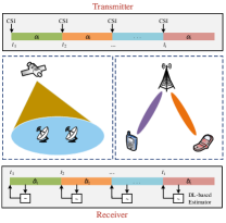
As shown by Fig. 2, in the proposed VPR transmission system, the transmitter changes the symbol packing ratio at every specific moment, which divides the transmitted symbols into different segments and results in individual transmission rates within each part. The determination of each packing ratio is based on CSI, cooperative target or other possible strategies. Different from the conventional variable coding and modulation (VCM) schemes [28], the receiver in the proposed VPR system does not need to know precisely the current symbol packing ratio. The only necessary knowledge is when the parameter changes, which can be appointed in advance. Then, the DL-based estimation will help the receiver infer the packing ratio within a short time.

There are two advantages to employ intelligent estimation for $\alpha$ in the receiver instead of directly sending it by the transmitter. Considering high SE, since no control message is required, the proposed VPR conducts negligible modification to the existing communication paradigms (e.g., spectrum allocation or frame structure). Also, when considering security, if $\alpha$ is put into the frame head, the repeated specific modulation type and UW word will make it easy for the eavesdropper to locate and decode the information.

III-B VPR-based Transmission for High SE

In this scenario, the packing ratio should be determined to balance the SE and the performance constraint (e.g., BER or ISI strength). For example, the SNR where $BER=10^{-3}$ can be employed as the threshold to select the packing ratio to achieve the maximum SE with acceptable BER performance, as demonstrated in Section VII. Also, the signal-to-interference-plus-noise ratio (SINR) can be applied for the base station and satellite to adjust the packing ratio in non-orthogonal multiple access (NOMA) which divides users into pairs and the multi-beam satellite serving users within a certain area.

The positions when the packing ratio changes can be generated by the following approaches.

1.

Fixed interval. After the synchronization, the transmitter checks the transmission status after every fixed interval and decides whether to change the packing ratio. The receiver should carry out the estimation at the same positions.
2.

Static storage. A preset vector of starting positions is determined with the practical characteristics of the transmission environment and the requirement.
3.

Pilot or dedicated channel. Without considering security, a public object (e.g., dedicated channel or pilot) can directly carry the information of packing ratio, at the expense of extra resources consumed and the modification of existing resources allocation.

III-C VPR-based Secure Transmission

The VPR-based transmission is a promising paradigm to improve the security of communications. For one thing, the change of the symbol packing ratio only affects the baseband symbols and can not be caught by analysis of the frequency spectrum. For another, the blind estimation cannot indicate the accurate starting position. Once the eavesdropper employs a wrong symbol packing ratio, the sampled points will severely deviate from their correct positions, making it meaningless to detect the signals and further estimate the following symbol packing ratio.

In this scenario, the packing ratio should be employed randomly with the same probability to avoid possible detection and attack, as assumed for the roll-off factors in [27]. The positions when the packing ratio changes can be generated by the following approaches.

1.

Static storage. A preset vector of starting positions should be stored in advance. Although such assumptions have been widely employed [27], it suffers from the risk that the expected security will disappear once the information is stolen by the eavesdropper.
2.

Dynamic generation. A dynamic generation can effectively avoid the risk resulting from information leakage. In this paper, we utilize the fact that the CSI is known only by the two sides of communications and propose a dynamic scheme to generate a secret sequence of starting positions. The following section will give a detailed introduction on it.

IV The Proposed Dynamic Generation Scheme for Positions of Segments

IV-A The Architecture of the Dynamic Generation Scheme

This section presents the proposed dynamic generation scheme for the starting positions of each segment where a new packing ratio is employed. The architecture of the scheme is shown in Fig. 3. Alice, Bob, and Eve represent the transmitter, the receiver and the eavesdropper, respectively. The detailed steps are presented as follows.

•

Channel measurement. In this stage, the two sides of communications send pilots to each other to measure the channel characteristics (e.g., signal intensity or channel response).
•

Quantization. In this step, the transmitter and receiver quantize the measured information into a bit sequence by single [29], double [30] or multiple-threshold [31] quantization.
•

Information reconciliation. This step is conducted to correct the errors between the quantized bit sequence of the transceivers. For example, in Cascade-based information reconciliation [32], Alice splits the bits into segments and sends parity check information to Bob. Bob checks the parity states with corresponding pieces. Once the parity bits mismatch, a binary search is conducted by changing as few bits as possible to satisfy the parity requirement.
•

Privacy amplification. Generally speaking, there always exists some information that leaks to Eve in the information reconciliation stage. By mapping the quantized information into a new bit sequence (i.e., the secret key) with the hash function (e.g., the message-digest algorithm 5 (MD5)), the risk resulting from the partly leaked information can be eliminated.
•

Pseudo-noise (PN) sequence generation. In this step, the secret key is employed as the seed for the PN generator, which can produce random and unrelated bits within its period.
•

Position calculation. The offsets can be easily obtained by splitting the PN sequence into segments with the same length and transforming them into signed integers. Then, the starting positions can be calculated by adding them to the original positions with the fixed step.

IV-B Performance Analysis for the Dynamic Generation Scheme

1.

Security. The CSI between Alice and Bob can only be measured by both of them, Eve cannot obtain it even if the pilot is eavesdropped. Except the information reconciliation, the other stages are safe since they are executed internally without any information exchanged.

Although limited information may be leaked by the parity sent to Bob, the hash mapping operation enhances the system security by mapping the information bits to a new bit sequence (i.e., the secret key) which cannot be inferred by partial original information.

So, throughout this paper, the private key, as well as the generated positions, are considered to be secret and cannot be obtained by Eve.
2.

Randomness. In fact, this issue has been studied in the physical layer security field. The national institute of standards and technology (NIST) test [33] is widely employed to measure the randomness of the generated secret key. There have been many existing CSI-based key generation schemes that pass the NIST test.
3.

Robustness. Another import metric is the robustness, which means the proposed scheme can work well under various scenarios and guarantee enough randomness.

The work about this issue can also be found in the existing literature. For example, the secret key generation under different transmission, e.g., MIMO [34] and multi-carrier communications [35], have been widely studied. The solution in different channels (e.g., multi-path channel [36] and even the static channel [31, 35]) have also been presented.
4.

Period. The PN generator has a period of $2^{N_{r}}$ , where $N_{r}$ is the number of the registers (i.e., the number of bits in the PN generator’s state). During the period, the generated bits has an excellent autocorrelation feature which achieves nearly an impulse function. When the generated bits are divided by step $N_{s}$ , the period of the calculated offset is $\rm lcm(2^{N}_{r},N_{s})$ , where ${\rm lcm}(a,b)$ means the least common multiple of $a$ and $b$ .

V A Simplified Symbol Packing Ratio Estimation for FTN Signaling

In this part, we present a simplified symbol packing ratio estimation for FTN signaling. Fig. 4 illustrates the complete architecture of the proposed estimation. The symbols that have passed through the matched filter and then been sampled are applied as the input of several analysis models. The main task of the analysis for $\alpha_{k}$ is to decide whether $\alpha=\alpha_{k}$ , where $\alpha$ is the correct symbol packing ratio employed by the transmitter.

Fig. 5 shows the detailed structure of the branch for analyzing whether $\alpha=\alpha_{k}$ . Firstly, the input symbols are down-sampled by the shared knowledge of starting position and interval $\alpha_{i}T_{N}$ . Then, through serial-parallel conversion (S/P), the sampled serial symbols are reformed and fed into the deep neural network (DNN) [37]. The output of DNN can be regarded as the probability of $\alpha_{A}=\alpha_{k}$ and will be transformed into integer 0 (false) or 1 (true). And finally, the number of true decisions during a specific time will be counted.

The DNN we employed in Fig. 5 contains an input layer, three hidden layers and an output layer. Each hidden layer is a sparsely connected layer with ReLU as its activation function. The system function of the DNN can be written as

\mathbf{y}=g_{4}\left(f\left(g_{3}\left(f\left(g_{2}\left(f\left(g_{1}(\bm{x})\right)\right)\right)\right)\right)\right.,

(4)

where $f(\bm{x})_{i}=\max\left(x_{i},0\right)$ is the item-wise ReLU function to vector $\bm{x}$ . $g_{i}(\bm{x})=\bm{W}_{i}\bm{x}+\bm{b}_{i}$ , where $\bm{W}_{i}$ and $\bm{b}_{i}$ are the weight matrix and bias vector in the $i$ -th layer of the DNN.

Benefiting from that the information of starting position for each transmission segment with a new $\alpha$ is known by both the transceiver, the receiver does not need to divide the signal into several streams [38] to avoid the sampling offset. So, the multiplexer (MUX), the demultiplexer (DEMUX) and the decision model in the original structure can be removed.

Meanwhile, we focus on the simplification of DNN. The main idea is to reduce the amounts of items in the weight matrices. Here, we employ an iterative strategy. After the model is well trained, we remove the items in $\bm{W}_{i}$ that are small enough and then train the remaining network. The process will be iteratively carried out until the target sparsity ratio is reached.

VI Spectrum Efficiency of Proposed VPR System in Different Channels

Generally speaking, the proposed VPR-based system can work well on various channels as long as FTN signaling are applicable. Here, we consider the AWGN, Rayleigh [39] and Nakagami-m [40] channels as the examples. The Rayleigh and Nakagami-m channels are typical fading channels that were first studied in 1940s and 1960s, repectively.

VI-A Theoretical SE of VPR System in AWGN Channel

In the receiver, $\alpha$ can be easily obtained with the help of blind estimation and the exact starting position. So, $\alpha$ can be regarded as the shared information between the transmitter and the receiver. And the transmission can be considered to be a conventional FTN signaling. With power $\sigma_{s}^{2}=P_{s}\alpha T_{N}$ for the transmitted signal, the analytical-form capacity of FTN signaling can be been formulated by Rusek as [26]

R_{A}(\alpha)=\frac{1}{2\pi\alpha T_{N}}\int_{0}^{\pi}\log_{2}\left(1+\frac{2\sigma_{s}^{2}}{N_{B}}H(\alpha,\omega)\right)\rm d\omega,

(5)

where $N_{B}/2$ is the power spectrum density of the Gaussian noise in the AWGN channel. And $H(\alpha,\omega)$ is defined by

H(\alpha,\omega)=\frac{1}{\alpha T_{N}}\sum_{k=-\infty}^{\infty}\left|G\left(\frac{\omega}{2\pi\alpha T_{N}}+\frac{k}{\alpha T_{N}}\right)\right|^{2},

(6)

where $G(f)$ is the Fourier transform of $h(t)$ . $|G(f)|^{2}$ can be expressed as [41]

|G\left(f\right)|^{2}=\begin{cases}T_{N},&|f|\in\left[0,\frac{1-\beta}{2T_{N}}\right]\\ \frac{T_{N}}{2}\left\{1+\cos\left[\frac{\pi T_{N}}{\beta}\left(\left|f\right|-\frac{1-\beta}{2T_{N}}\right)\right]\right\},&|f|\in\left[\frac{1-\beta}{2T_{N}},\frac{1+\beta}{2T_{N}}\right]\\ 0,&|f|\in\left[\frac{1+\beta}{2T_{N}},+\infty\right]\\ \end{cases}.

(7)

Here, we define three bound functions $b_{1}\left(\alpha\right)={\alpha\pi(1-\beta)}$ , ${b_{2}}\left(\alpha\right)=2\pi-\alpha\pi\left({1+\beta}\right)$ and ${b_{3}}\left({\alpha}\right)=\alpha\pi\left(1+\beta\right)$ . And the following conclusion can be derived.

Lemma 1

When $\omega\in[0,\pi]$ , for any $k\geq 1$ , it always holds that

G^{2}\left(\frac{\omega+2k\pi}{2\pi\alpha T_{N}}\right)=0.

(8)

Proof:

Here, we firstly assume that for any $k\geq 1$ , it holds that

\frac{\omega+2\pi k}{2\pi\alpha T_{N}}\geq\frac{1+\beta}{2T_{N}}.

(9)

Since that $\omega\in[0,\pi]$ , (9) can be proved by

\frac{\omega+2\pi k}{2\pi\alpha T_{N}}\geq\frac{1+\beta}{2T_{N}}\Leftarrow\frac{2\pi k}{2\pi\alpha T_{N}}\geq\frac{1+\beta}{2T_{N}}\Leftrightarrow\frac{k}{\alpha}\geq\frac{1+\beta}{2}\Leftrightarrow 2k\geq\alpha(1+\beta).

(10)

Considering that $k>1$ and $0\leq\alpha,\beta\leq 1$ , (10) can be further obtained by

2k\geq\alpha(1+\beta)\Leftarrow 2\geq\alpha\left(1+\beta\right)\Leftarrow 2\geq 2.

(11)

It’s obviously that $2>2$ always holds. So, the assumption (9) is proved. And finally, Lemma 1 can be proved by combining (7) with (9). ∎

Lemma 2

When $\omega\in[0,\pi]$ , for any $k\leq-2$ , it always holds that

G^{2}\left(\frac{\omega+2k\pi}{2\pi\alpha T_{N}}\right)=0.

(12)

Proof:

Firstly, we assume that for any $k\leq-2$ , it holds that

\frac{\omega+2\pi k}{2\pi\alpha T_{N}}\leq-\frac{1+\beta}{2T_{N}}.

(13)

Since that $\omega\in[0,\pi]$ , (13) can be proved by

\displaystyle\frac{\omega+2\pi k}{2\pi\alpha T_{N}}\leq-\frac{1+\beta}{2T_{N}}\Leftarrow\frac{\pi+2\pi k}{2\pi\alpha T_{N}}\leq-\frac{1+\beta}{2T_{N}}\Leftrightarrow 2k\leq-\alpha\left(1+\beta\right)-1.

(14)

Considering that $k\leq-2$ and $0\leq\alpha,\beta\leq 1$ , (14) can be obtained by

2k\leq-\alpha\left(1+\beta\right)-1\Leftarrow-4\leq-\alpha\left(1+\beta\right)-1\Leftarrow-4\leq-3.

(15)

It’s obviously that $-4\leq-3$ always holds. So, (13) is proved. And finally, Lemma 2 can be proved by combining (7) with (13). ∎

Theorem 1

For $\omega\in[0,\pi]$ , $H(\alpha,\omega)$ can be expressed as

H(\alpha,\omega)=\frac{1}{\alpha T_{N}}\;\left(G^{2}\left(\frac{\omega}{2\pi\alpha\mathrm{T}_{N}}\right)+G^{2}\left(\frac{\omega-2\pi}{2\pi\alpha\mathrm{T}_{N}}\right)\;\right).

(16)

Proof:

The theorem can be proved by combining Lemma 1, Lemma 2 and (6). ∎

Lemma 3

For $\omega\in\left[0,b_{1}(\alpha)\right)$ , it always holds that

H(\alpha,\omega)=\frac{1}{\alpha}.

(17)

Proof:

Since that $\omega\in[0,b_{1}(\alpha))$ , it can be obtained that

0\leq\frac{\omega}{2\pi\alpha T_{N}}\leq\frac{b_{1}(\alpha)}{2\pi\alpha T_{N}}=\frac{1-\beta}{2T_{N}}.

(18)

Considering (7) and (18), for $\omega\in[0,b_{1}(\alpha))$ , it can be derived that

G^{2}\left(\frac{\omega}{2\pi\alpha T_{N}}\right)=\frac{1}{\alpha}.

(19)

Also, since $\omega\in[0,b_{1}(\alpha)$ , it can be obtained that

\frac{\omega-2\pi}{2\pi\alpha T_{N}}\leq\frac{b_{1}(\alpha)-2\pi}{2\pi\alpha T_{N}}=\frac{\alpha\pi\left(1-\beta\right)-2\pi}{2\pi\alpha T_{N}}.

(20)

Considering that $0\leq\alpha,\beta\leq 1$ , (20) can be further written as

\frac{\omega-2\pi}{2\pi\alpha T_{N}}\leq\frac{\alpha\pi\left(1-\beta\right)-2\pi}{2\pi\alpha T_{N}}\leq\frac{\alpha\pi\left(1-\beta\right)-2\alpha\pi}{2\pi\alpha T_{N}}=-\frac{1+\beta}{2T_{N}}.

(21)

Considering (7) and (21), it can be derived that

G^{2}\left(\frac{\omega-2\pi}{2\pi\alpha T_{N}}\right)=0.

(22)

Finally, Lemma 3 can be proved by combining Theorem 1, (19) and (22). ∎

Lemma 4

For $\omega\in[b_{3}(\alpha),\pi]$ and $b_{2}(\alpha)\geq\pi$ , it always holds that

G^{2}\left(\frac{\omega}{2\pi\alpha T_{N}}\right)=0.

(23)

Proof:

Firstly, it can be obtained by $b_{2}(\alpha)\geq\pi$ that

b_{2}\left(\alpha\right)=2\pi-\alpha\pi\left(1+\beta\right)\geq\pi\\ \Leftrightarrow\alpha\leq\frac{1}{1+\beta}.

(24)

Then, since that $\omega\in[b_{3}(\alpha),\pi]$ , it can be obtained that

\frac{\omega-2\pi}{2\pi\alpha T_{N}}\leq\frac{\pi-2\pi}{2\pi\alpha T_{N}}=-\frac{1}{2\alpha T_{N}}\leq-\frac{1+\beta}{2T_{N}}.

(25)

Considering (7) and (25), it can be derived that

G^{2}\left(\frac{\omega-2\pi}{2\pi\alpha T_{N}}\right)=0.

(26)

Also, since that $\omega\in[b_{3}(\alpha),\pi]$ , it can be obtained that

\frac{\omega}{2\pi\alpha T_{N}}\geq\frac{\alpha\pi\left(1+\beta\right)}{2\pi\alpha T_{N}}=\frac{1+\beta}{2T_{N}}.

(27)

Considering (7) and (27), it can be derived that

G^{2}\left(\frac{\omega}{2\pi\alpha T_{N}}\right)=0.

(28)

Finally, Lemma 4 can be proved by combining Theorem 1, (26) and (28). ∎

By combining Theorem 1, Lemma 3 and Lemma 4, $H(\alpha,\omega)$ can be expressed as

H\left(\alpha,\omega\right)=\begin{cases}H_{1}\left(\alpha,\omega\right),&b_{2}(\alpha)<\pi\\ H_{2}\left(\alpha,\omega\right),&b_{2}\left(\alpha\right)\geq\pi\\ \end{cases},

(29)

where

H_{1}\left(\alpha,\omega\right)=\begin{cases}\frac{1}{\alpha},&\omega\in\left[0,b_{1}\left(\alpha\right)\right)\\ \frac{1}{\alpha T_{N}}\;\left(G^{2}\left(\frac{\omega}{2\pi\alpha\mathrm{T}_{N}}\right)+G^{2}\left(\frac{\omega-2\pi}{2\pi\alpha\mathrm{T}_{N}}\right)\;\right),&\omega\in\left[b_{1}\left(\alpha\right),\pi\right]\\ \end{cases},

(30)

H_{2}\left(\alpha,\omega\right)=\begin{cases}\frac{1}{\alpha},&\omega\in\left[0,b_{1}\left(\alpha\right)\right)\\ \frac{1}{\alpha T_{N}}\;\left(G^{2}\left(\frac{\omega}{2\pi\alpha\mathrm{T}_{N}}\right)\;\right),&\omega\in\left[b_{1}\left(\alpha\right),b_{3}\left(\alpha\right)\right)\\ 0,&\omega\in\left[b_{3}\left(\alpha\right),\pi\right]\\ \end{cases}.

(31)

With the system bandwidth that can be calculated by $W=1/(2T_{N})=W_{T}/(1+\beta)$ , where $W_{T}$ is the total bandwidth of the channel, SE of FTN signaling can be written as

C_{A}(\alpha)=\frac{1}{\pi\alpha(1+\beta)}\underset{C_{B}\left(\alpha\right)}{\underbrace{\int_{0}^{\pi}{\log_{2}}\left(1+\frac{2\sigma_{s}^{2}}{N_{B}}H(\alpha,\omega)\right)\mathrm{d\omega}}}.

(32)

Then, we split $C_{B}\left(\alpha\right)$ into several subsection integral and calculate them respectively. For $\omega\in\left[0,b_{1}\left(\alpha\right)\right)$ , the integral can be expressed as

\begin{split}{C_{1}}\left(\alpha\right)=\int_{0}^{{b_{1}}\left(\alpha\right)}{{{\log}_{2}}\left({1+\frac{{2\sigma_{s}^{2}}}{{{N_{B}}}}H(\alpha,\omega)}\right)}{\rm{d}}\omega\vspace{1em}=\alpha\pi\left({1-\beta}\right){\log_{2}}\left({1+\frac{{2\sigma_{s}^{2}}}{{{\alpha N_{B}}}}}\right)\end{split}.

(33)

Theorem 2

(Chebyshev-Gauss Quadrature Rule) For a given function $f(x)$ , its integration between -1 and 1 can be approximated as [42]

\int_{-1}^{1}{\frac{f\left(x\right)}{\sqrt{1-x^{2}}}dx\approx\sum_{i=1}^{n}{w_{i}f\left(\xi_{i}\right)}},

(34)

where $\xi_{i}=\cos\left(\frac{2i-1}{2n}\pi\right)$ and $w_{i}=\frac{\pi}{n}$ .

Theorem 3

For given function $f(x)$ , its integration between $a$ and $b$ can be approximated as

\int_{a}^{b}{f}(x)\,dx\approx\frac{b-a}{2}\sum_{i=1}^{n}{w_{i}}\sqrt{1-\xi_{i}^{2}}f\left(\frac{b-a}{2}\xi+\frac{b+a}{2}\right),

(35)

where the values of $\xi_{i}$ and $w_{i}$ are the same as those in Theorem 2.

Proof:

Here, we set $x=\frac{b-a}{2}\xi+\frac{b+a}{2}$ . Then, the integration of $f(x)$ can be rewritten as

	$\displaystyle\int_{a}^{b}{f\left(x\right)dx}$	$\displaystyle=\int_{arg_{\xi}\left(a\right)}^{arg_{\xi}\left(b\right)}{f\left(\frac{b-a}{2}\xi+\frac{b+a}{2}\right)d\left[\frac{b-a}{2}\xi+\frac{b+a}{2}\right]}$		(36)
		$\displaystyle=\frac{b-a}{2}\int_{-1}^{1}{f\left(\frac{b-a}{2}\xi+\frac{b+a}{2}\right)d\xi}=\frac{b-a}{2}\int_{-1}^{1}{\frac{\sqrt{1-x^{2}}\psi\left(\xi\right)}{\sqrt{1-x^{2}}}d\xi},$		(36)

where $\psi(\xi)$ is defined as $\psi\left(\xi\right)=f\left(\frac{b-a}{2}\xi+\frac{b+a}{2}\right)$ .

Considering Theorem 2, (36) can be written as

\displaystyle\int_{a}^{b}{f\left(x\right)dx}

\displaystyle\approx\frac{b-a}{2}\sum_{i=1}^{n}{w_{i}\sqrt{1-{\xi_{i}}^{2}}\psi\left(\xi_{i}\right)}=\frac{b-a}{2}\sum_{i=1}^{n}{w_{i}\sqrt{1-{\xi_{i}}^{2}}f\left(\frac{b-a}{2}\xi_{i}+\frac{b+a}{2}\right)}.

(37)

∎

According to the Theorem 3, for $\omega\in\left[b_{1}\left(\alpha\right),\pi\right]$ , the integral can be written as

C_{2}\left(\alpha\right)=\int_{b_{1}\left(\alpha\right)}^{\pi}{\log_{2}\left(1+\frac{2\sigma_{s}^{2}}{N_{B}}H(\alpha,\omega)\right)d\omega}\approx A_{1}\sum_{i=1}^{N}{m_{i}\sqrt{1-\omega_{1i}^{2}}}\log_{2}\left(1+\frac{2\sigma_{s}^{2}}{N_{B}}H(\alpha,\omega_{1i})\right),

(38)

where $A_{1}=\frac{{\pi\left[{1{\rm{+}}\alpha{\mkern 1.0mu}\left({\beta-1}\right)}\right]{\mkern 1.0mu}}}{2}$ , $m_{i}=\frac{{\pi\left|{\sin\left({\frac{{\pi\left({2i-1}\right)}}{{2N}}}\right)}\right|}}{N}$ and ${\omega_{1i}}=\frac{\pi}{2}\left\{{\left[{1+\alpha\left({\beta-1}\right)}\right]\cos\left({\frac{{\pi(2i-1)}}{{2n}}}\right)+{1-\alpha\left({\beta-1}\right)}}\right\}$ .

Similarly, for $\omega\in\left[b_{1}\left(\alpha\right),b_{3}\left(\alpha\right)\right)$ , the integral can be written as

C_{3}\left(\alpha\right)=\int_{b_{1}(\alpha)}^{b_{3}(\alpha)}{\mathrm{l}_{2}}\left(1+\frac{2\sigma_{s}^{2}}{N_{B}}H(\alpha,\omega)\right)d\omega\approx A_{2}\sum_{i=1}^{N}{m_{i}}\sqrt{1-\omega_{2i}^{2}}\log_{2}\left(1+\frac{2\sigma_{s}^{2}}{N_{B}}H(\alpha,\omega_{2i})\right),

(39)

where $A_{2}=\pi\alpha\beta$ and ${\omega_{2i}}=\pi{\mkern 1.0mu}\alpha\left({1+\beta{\mkern 1.0mu}{\rm{cos}}\left({\frac{{\pi{\mkern 1.0mu}\left({2{\mkern 1.0mu}{i}-1}\right)}}{{2{\mkern 1.0mu}n}}}\right)}\right).$

For the convenience of implementation, the set of available $\alpha$ values is usually finite. Finally, for a specific $\alpha$ value, SE of the proposed VPR system in the AWGN channel can be written as

C_{A}\left(\alpha\right)=\left\{\begin{matrix}\frac{1}{\alpha\pi\left(1+\beta\right)}\left(C_{1}\left(\alpha\right)+C_{2}\left(\alpha\right)\right),&b_{2}\left(\alpha\right)<\pi\\ \frac{1}{\alpha\pi\left(1+\beta\right)}\left(C_{1}\left(\alpha\right)+C_{3}\left(\alpha\right)\right),&b_{2}\left(\alpha\right)\geq\pi\\ \end{matrix}\right..

(40)

To avoid the possible detection and attack when the VPR system is employed to improve the security, every $\alpha$ is preferred to be applied with the same probability, just as the roll-off factor in [27]. So, for the proposed VPR system, the average SE in such a scenario can be written as

C_{A}^{\prime}=\frac{1}{N_{\alpha}}\sum_{i=1}^{N_{\alpha}}C_{A}(\alpha_{i}),

(41)

where $\alpha_{i}$ ( $i=1,2\cdots,N_{\alpha}$ ) is the $i$ -th symbol packing ratio that is employed in the transmission.

VI-B Theoretical SE of VPR System in Rayleigh Channel

For the Rayleigh and Nakagami-m channel, the channel gain is considered and can be regarded as a constant during every data block in this paper. So, the power of the signal in the receiver with channel gain $h$ can be written as

\sigma_{s^{\prime}}^{2}\left(h\right)=h^{2}P_{s}\alpha T_{N}.

(42)

The capacity of FTN signaling with specific $h$ can be obtained as

R^{\prime}(\alpha)=\frac{1}{2\pi\alpha T_{N}}\int_{0}^{\pi}\log_{2}\left(1+\frac{2\sigma_{s^{\prime}}^{2}\left(h\right)}{N_{B}}H(\alpha,\omega)\right)\rm d\omega.

(43)

Considering that $h$ is a random variable, the mean SE of FTN signaling with packing ratio $\alpha$ in Rayleigh channel can be formulated as

\begin{split}C_{R}(\alpha)=\frac{1}{{\pi\alpha\left(1+\beta\right)}}\int_{0}^{\pi}{\underbrace{\int_{0}^{+\infty}{f_{R}(h)\cdot{\rm{lo}}{{\rm{g}}_{2}}\left({1+\frac{{2{h^{2}}P_{s}\alpha{T_{N}}}}{{{N_{B}}}}H(\alpha,\omega)}\right){{\rm d}h}}}_{{C_{i1}}(\alpha,\omega)}}{\rm{d\omega}}\end{split},

(44)

where $f_{R}(h)$ is the probability density function (PDF) of $h$ , which can be written as [39]

f_{R}(h)=\frac{h}{\sigma^{2}}e^{-\frac{h^{2}}{2\sigma^{2}}},

(45)

where $\sigma^{2}$ is the power parameter. Then, by applying $C_{o1}(\alpha,\omega)=2P_{s}\alpha T_{N}H\left(\alpha,\omega\right)/N_{B}$ , $C_{i1}\left(\alpha,\omega\right)$ , which has been defined in (44), can be written as

\begin{split}&{C_{i1}}(\alpha,\omega)=\int_{0}^{+\infty}{{\rm{-lo}}{{\rm{g}}_{2}}\left({1+{C_{o1}(\alpha,\omega)}{h^{2}}}\right)\left({-\frac{h}{{{\sigma^{2}}}}{e^{-\frac{{{h^{2}}}}{{2{\sigma^{2}}}}}}}\right){\rm{d}}h}.\end{split}

(46)

By extracting the integral items as $F_{1}(\alpha,\omega)=-{\rm log}_{2}\left(1+C_{o1}\left(\alpha,\omega\right)h^{2}\right)$ and $F_{2}(h)=e^{\frac{-h^{2}}{2\sigma^{2}}}$ , $C_{i1}(\alpha,\omega)$ can be expressed as

{C_{i1}}(\alpha,\omega)=\int_{0}^{+\infty}{{F_{1}}(h,\alpha,\omega){F_{2}}^{\prime}(h){\rm d}h}.

(47)

According to the principle of integral by parts [43], $C_{i}(h,\alpha,\omega)$ can be further written as

\begin{split}C_{i1}\left(\alpha,\omega\right)=&{F_{1}}\left(h,\alpha,\omega\right){F_{2}}\left(h\right)\left|{{}_{0}^{+\infty}}\right.-\int_{0}^{+\infty}{F_{1}}^{\prime}\left(h,\alpha,\omega\right){F_{2}}\left(h\right){\rm{d}}h.\end{split}

(48)

Due to the fact that

F_{1}(0,\alpha,\omega)F_{2}(0)=-{\rm log2}(1)\cdot e^{0}=0,

(49)

\begin{split}\mathop{\lim}\limits_{h\to+\infty}{F_{1}}(h,\alpha,\omega)F_{2}(h)=\mathop{\lim}\limits_{h\to+\infty}\left({-{{\log}_{2}}\left({1+{C_{o1}}\left({\alpha,\omega}\right){h^{2}}}\right){e^{\frac{{-{h^{2}}}}{{2{\sigma^{2}}}}}}}\right)=0,\end{split}

(50)

(48) can be expressed as

\begin{split}&{C_{i1}}\left(\alpha,\omega\right)=-\int_{0}^{+\infty}{\frac{{2{C_{o1}}\left({\alpha,\omega}\right)h}}{{\ln 2\cdot\left({1+{C_{o1}}\left({\alpha,\omega}\right){h^{2}}}\right)}}}{e^{-\frac{{{h^{2}}}}{{2{\sigma^{2}}}}}}{\rm{d}}h\\ {\rm{=}}&-\frac{{\rm{e}}^{\frac{1}{{2\sigma^{2}{C_{o1}}\left({\alpha,\omega}\right)}}}}{\ln 2}\int_{\frac{1}{2\sigma^{2}C_{o1}\left(h,\alpha,\omega)\right)}}^{+\infty}{\frac{2\sigma^{2}{e^{-\frac{{\frac{1}{{{C_{o1}}\left({\alpha,\omega}\right)}}+{h^{2}}}}{{2{\sigma^{2}}}}}}}{{\left({\frac{1}{{{C_{o1}}\left({\alpha,\omega}\right)}}+{h^{2}}}\right)}}}d\left({\frac{{\frac{1}{{{C_{o1}}\left({\alpha,\omega}\right)}}+{h^{2}}}}{2\sigma^{2}}}\right)\\ &{\rm{=}}-\frac{{{e^{\frac{{{N_{B}}}}{{4{\sigma^{2}}P_{s}\alpha{T_{N}}H(\alpha,\omega)}}}}}}{{\ln 2}}{\rm Ei}\left(-{\frac{{{N_{B}}}}{{4\sigma^{2}P_{s}\alpha{T_{N}}H(\alpha,\omega)}}}\right),\end{split}

(51)

where ${\rm E_{i}}(x)$ is the exponential integral function which is defined as ${\rm E_{i}}(x)=\int_{-x}^{+\infty}{\frac{{{e^{-t}}}}{t}\rm d}t$ .

Now, by applying ${C_{o2}}\left(\alpha\right)=-4\sigma^{2}P_{s}\alpha{T_{N}}/{N_{B}}$ , (44) can be written as

{C_{R}}(\alpha)=-\frac{1}{{\pi\alpha\left({1+\beta}\right)\ln 2}}\underbrace{\int_{0}^{\pi}{{e^{-\frac{{{C_{o2}}\left(\alpha\right)}}{{H(\alpha,\omega)}}}}}{\rm{Ei}}\left({\frac{{{C_{o2}}}}{{H(\alpha,\omega)}}}\right)d\omega}_{{C_{i2}}\left(\alpha,\omega\right)}.

(52)

Then, we split $C_{i2}\left(\alpha,\omega\right)$ into several subsection integral and calculate them respectively. For $\omega\in\left[0,b_{1}\left(\alpha\right)\right)$ , the integral can be calculated as

\begin{split}{C_{4}}\left({\alpha}\right)&=\int_{0}^{{b_{1}}\left(\alpha\right)}{{e^{-\frac{{{C_{o2}}(\alpha)}}{{H(\alpha,\omega)}}}}}{\mathop{\rm Ei}\nolimits}\left({\frac{{{C_{o2}}}}{{H(\alpha,\omega)}}}\right)d\omega=\int_{0}^{{b_{1}}\left(\alpha\right)}{{e^{-\alpha C_{o2}\left(\alpha\right)}}{\rm{Ei}}\left({{\alpha}{C_{o2}}\left(\alpha\right)}\right)d\omega}\vspace{1em}\\ &=\alpha\pi\left({1-\beta}\right){e^{-{\alpha}{C_{o2}}}}{\rm{Ei}}\left({\alpha{C_{o2}}\left(\alpha\right)}\right).\end{split}

(53)

According to the Theorem 3, for $\omega\in\left[b_{1}\left(\alpha\right),\pi\right]$ , the integral can be written as

C_{5}\left(\alpha\right)=\int_{b_{1}\left(\alpha\right)}^{\pi}{e^{-\frac{C_{o2}(\alpha)}{H(\alpha,\omega)}}\mathrm{Ei}\left(\frac{C_{o2}}{H(\alpha,\omega)}\right)d\omega}\approx A_{1}\sum_{i=1}^{N}{m_{i}}\sqrt{1-\omega_{1i}^{2}}e^{-\frac{C_{o2}(\alpha)}{H(\alpha,\omega_{1i})}}\mathrm{Ei}\left(\frac{C_{o2}}{H(\alpha,\omega_{1i})}\right).

(54)

Similarly, for $\omega\in\left[b_{1}\left(\alpha\right),b_{3}\left(\alpha\right)\right)$ , the integral can be written as

C_{6}\left(\alpha\right)=\int_{b_{1}(\alpha)}^{b_{3}(\alpha)}{e^{-\frac{C_{O}(\alpha)}{H(\alpha,\omega)}}}\mathrm{Ei}\left(\frac{C_{o2}}{H(\alpha,\omega)}\right)d\omega\approx A_{2}\sum_{i=1}^{N}{m_{i}\sqrt{1-\omega_{2i}^{2}}}e^{-\frac{C_{a2}(\alpha)}{H\left(\alpha,\omega_{2i}\right)}}\mathrm{Ei}\left(\frac{C_{o2}}{H\left(\alpha,\omega_{2i}\right)}\right).

(55)

Finally, the SE of the proposed VPR scheme in Rayleigh channel can be written as

C_{R}\left(\alpha\right)=\left\{\begin{matrix}\frac{1}{\alpha\pi\left(1+\beta\right)}\left(C_{4}\left(\alpha\right)+C_{5}\left(\alpha\right)\right),&b_{2}\left(\alpha\right)<\pi\\ \frac{1}{\alpha\pi\left(1+\beta\right)}\left(C_{4}\left(\alpha\right)+C_{6}\left(\alpha\right)\right),&b_{2}\left(\alpha\right)\geq\pi\\ \end{matrix}\right..

(56)

The average SE for VPR-based secure transmission in Rayleigh channel can be obtained as

C_{R}^{\prime}=\frac{1}{N_{\alpha}}\sum_{i=1}^{N_{\alpha}}C_{R^{\prime}}(\alpha_{i}).

(57)

VI-C Theoretical SE of VPR System in Nakagami-m Channel

Similar to (44), the SE of FTN signaling in Nakagami-m channel can be formulated as

\begin{split}{C_{N}}(\alpha)=\frac{1}{{\pi\alpha\left({1+\beta}\right)}}\cdot\int_{0}^{\pi}{\underbrace{\int_{0}^{+\infty}{f_{N}\left(h\right)\cdot{\rm{lo}}{{\rm{g}}_{2}}\left({1+\frac{{2{h^{2}}P_{s}\alpha{T_{N}}}}{{{N_{B}}}}H(\alpha,\omega)}\right){\rm{d}}h}}_{{C_{i2}}(\alpha,\omega))}}{\rm{d}}\omega\end{split},

(58)

where $f_{N}\left(h\right)$ is the PDF of $h$ in Nakagami-m channel which can be written as [40]

{f_{N}}\left(h\right)=\frac{{2{m^{m}}{h^{2m-1}}}}{{\Gamma\left(m\right){P_{r}}^{m}}}{e^{-\frac{{m{h^{2}}}}{{{P_{r}}}}}},

(59)

where $m$ ( $m>0$ ) is the fading parameter , $P_{r}$ is the average power, $\Gamma\left(m\right)$ is the Gamma function which can be expressed as [44]

\Gamma(m)=\int_{0}^{+\infty}{{t^{m-1}}}{e^{-t}}\;{\rm{d}}t\quad(m>0).

(60)

By applying ${C_{o3}}={2{m^{m}}}/\left(\Gamma\left(m\right)P_{r}^{m}\right)$ , the integral of channel gain $h$ can be written as

\begin{split}{C_{i,2}}\left({\alpha,\omega}\right)\vspace{1em}&=\int_{0}^{+\infty}{{{\rm{C}}_{o3}}{{\rm{h}}^{2m-1}}{e^{-\frac{{m{h^{2}}}}{{{P_{r}}}}}}{\rm{lo}}{{\rm{g}}_{2}}\left({1+{C_{o1}}\left({\alpha,\omega}\right){h^{2}}}\right){\rm{d}}h}\vspace{1em}\\ &={C_{o3}}{\cal M}\left[{{e^{-\frac{{m{h^{2}}}}{{{P_{r}}}}}}{\rm{lo}}{{\rm{g}}_{2}}\left({1+{C_{o1}}\left({\alpha,\omega}\right){h^{2}}}\right);2m}\right],\end{split}

(61)

where $\mathcal{M}\left[f\left(x\right);s\right]$ means the Mellin transform [45] of ${f\left(x\right)}$ .

Theorem 4

(Mellin Convolution Theorem) For functions $f(x)$ and $g(x)$ , it holds that

\mathcal{M}\left[f(x)g(x);s\right]=\frac{1}{2\pi i}\!\int_{c\!-\!i\infty}^{c+i\infty}{\mathcal{M}\left[f\left(x\right);s\right]\mathcal{M}\left[g\left(x\right);s-u\right]du}.

(62)

Considering Theorem 4, (61) can be further written as

\displaystyle C_{i,2}\left(\alpha,\omega\right)=\frac{1}{2\pi i}\int_{c-i\infty}^{c+\infty}{\mathcal{M}\left[e^{-\frac{mh^{2}}{P_{r}}};2m-u\right]\mathcal{M}\left[\log_{2}\left(1+C_{o1}\left(\alpha,\omega\right)h^{2}\right);u\right]}du.

(63)

Property 1

The Mellin transform has the properties as follows [46].

	$\displaystyle\mathcal{M}\left[f\left(\nu x\right);s\right]=\nu^{-s}f^{*}\left(s\right),\,\,\nu>0,$		(64)
	$\displaystyle\mathcal{M}\left[e^{-x^{2}};s\right]=\frac{1}{2}\Gamma\left(\frac{s}{2}\right),\,\,\mathrm{Re}\left(s\right)>0,$		(65)
	$\displaystyle\mathcal{M}\left[f\left(x^{\nu}\right);s\right]=\frac{1}{\left\|\nu\right\|}f^{*}\left(\frac{s}{\nu}\right),\,\,s/\nu\,\,\mathrm{is}\,\,\mathrm{feasible},$		(66)
	$\displaystyle\mathcal{M}\left[\ln\left(1+x\right);s\right]=\frac{\pi}{s\sin\left(\pi s\right)},-1\leq\mathrm{Re}\left(s\right)\leq 0.$		(67)

Considering (64) and (65), it can be obtained that

\mathcal{M}\left[e^{-\frac{mh^{2}}{P_{r}}};2m-u\right]=\left(\frac{m}{P_{r}}\right)^{-\left(m-\frac{u}{2}\right)}\mathcal{M}\left[e^{-h^{2}};2m-u\right]=\frac{1}{2}\left(\frac{m}{P_{r}}\right)^{-\left(m-\frac{u}{2}\right)}\Gamma\left(m-\frac{u}{2}\right).

(68)

Considering (64), (66) and (67), it can be obtained that

	$\displaystyle\mathcal{M}\left[\log_{2}\left(1+C_{o1}\left(\alpha,\omega\right)h^{2}\right);u\right]$	$\displaystyle=\frac{1}{2\ln 2}\left[C_{o1}\left(\alpha,\omega\right)\right]^{-\frac{u}{2}}\mathcal{M}\left[\ln\left(1+h\right);\frac{u}{2}\right]$		(69)
		$\displaystyle=\frac{1}{\ln 2}\left[C_{o1}\left(\alpha,\omega\right)\right]^{-\frac{u}{2}}\frac{\pi}{u\sin\left(\frac{\pi u}{2}\right)}.$		(69)

Combining (68) and (69), (63) can be written as

C_{i,2}\left(\alpha,\omega\right)=\frac{C_{o,3}}{2\pi i}\int_{c-i\infty}^{c+i\infty}{\frac{\pi\left(\frac{P_{r}}{m}\right)^{m-\frac{u}{2}}\Gamma\left(m-\frac{u}{2}\right)}{4\ln 2\cdot\left(-\frac{u}{2}\right)\left[C_{o,1}\left(\alpha,\omega\right)\right]^{\frac{u}{2}}\sin\left(-\frac{\pi u}{2}\right)}}du.

(70)

Property 2

Gamma function has the properties as follows.

	$\displaystyle\Gamma\left(1-x\right)\Gamma\left(x\right)=\frac{\pi}{\sin\left(\pi x\right)},$		(71)
	$\displaystyle\Gamma\left(x+1\right)=x\Gamma\left(x\right).$		(72)

Considering Property 2, (70) can be further written as

$\displaystyle C_{i,2}\left(\alpha,\omega\right)=$	$\displaystyle\frac{C_{o,3}}{2\pi i}\int_{c-i\infty}^{c+i\infty}{\frac{\left(\frac{P_{r}}{m}\right)^{m-\frac{u}{2}}\Gamma\left(m-\frac{u}{2}\right)\Gamma\left(1+\frac{u}{2}\right)\Gamma\left(-\frac{u}{2}\right)\Gamma\left(-\frac{u}{2}\right)}{4\ln 2\cdot\Gamma\left(1-\frac{u}{2}\right)\cdot\left[C_{o,1}\left(\alpha,\omega\right)\right]^{\frac{u}{2}}}}du$	(73)
$\displaystyle=$	$\displaystyle\frac{C_{o,3}\left(\frac{P_{r}}{m}\right)^{m}}{2\ln 2}\cdot\frac{1}{2\pi i}\int_{c-i\infty}^{c+i\infty}{\frac{\Gamma\left(m-\frac{u}{2}\right)\Gamma\left(1+\frac{u}{2}\right)\Gamma\left(-\frac{u}{2}\right)\Gamma\left(-\frac{u}{2}\right)}{\Gamma\left(1-\frac{u}{2}\right)}}\left(\frac{m}{P_{r}C_{o1}\left(\alpha,\omega\right)}\right)^{\frac{u}{2}}d\left(\frac{u}{2}\right)$
$\displaystyle=$	$\displaystyle\frac{C_{o,3}\left(\frac{P_{r}}{m}\right)^{m}}{2\ln 2}\cdot G_{1,0}^{3,1}\left(\left.\begin{array}[]{c}0,1\\ 0,0,m\\ \end{array}\right\|\frac{m}{P_{r}C_{o1}\left(\alpha,\omega\right)}\right),$

where $G_{p,\;q}^{m,\;n}\left({\begin{array}[]{*{20}{c}}{{a_{1}},{a_{2}}\cdots{a_{p}}}\\ {{b_{1}},{b_{2}}\cdots{b_{q}}}\end{array}\left|z\right.}\right)$ represents the Meijer-G function [47].

By applying $C_{o4}={m{N_{B}}}/\left({2P_{s}\alpha{T_{N}}{P_{r}}}\right)$ , for $\omega\in\left[0,b_{1}(\alpha)\right)$ , the integral can be written as

\begin{split}{C_{7}}(\alpha)&=\int_{0}^{{b_{1}}(\alpha)}{\frac{1}{{\Gamma\left(m\right)\ln(2)}}\cdot G_{1,\;0}^{3,\;1}\left({\left.{\begin{array}[]{*{20}{c}}{0,1}\\ {0,0,m}\end{array}}\right|\alpha{C_{o4}}\left({\alpha,\omega}\right)}\right)}{\rm{d}}\omega\\ &=\frac{\alpha\pi\left(1-\beta\right)}{{\Gamma\left(m\right)\ln(2)}}\cdot G_{1,\;0}^{3,\;1}\left({\left.{\begin{array}[]{*{20}{c}}{0,1}\\ {0,0,m}\end{array}}\right|\alpha{C_{o4}}\left({\alpha,\omega}\right)}\right).\end{split}

(74)

For $\omega\in\left[b_{1}(\alpha),\pi\right)$ , the integral can be written as

	$\displaystyle C_{8}(\alpha)$	$\displaystyle=\int_{b_{1}(\alpha)}^{\pi}{\frac{1}{\Gamma\left(m\right)\ln\mathrm{(}2)}\cdot G_{1,\;0}^{3,\;1}\left(\begin{array}[]{c}0,1\\ 0,0,m\\ \end{array}\left\|\frac{C_{o4}}{H\left(\alpha,\omega\right)}\right.\right)}d\omega$		(75)
		$\displaystyle\approx\frac{C_{1}}{\Gamma\left(m\right)\ln\mathrm{(}2)}\sum_{i=1}^{N}{m_{i}}\sqrt{1-\omega_{1i}^{2}}\cdot G_{1,\;0}^{3,\;1}\left(\begin{array}[]{c}0,1\\ 0,0,m\\ \end{array}\left\|\frac{C_{o4}}{H\left(\alpha,\omega_{1i}\right)}\right.\right).$		(75)

And for $\omega\in\left[b_{1}(\alpha),b_{3}(\alpha)\right)$ , the integral can be written as

	$\displaystyle C_{9}(\alpha)$	$\displaystyle=\int_{b_{1}(\alpha)}^{b_{3}\left(\alpha\right)}{\frac{1}{\Gamma\left(m\right)\ln\mathrm{(}2)}\cdot G_{1,\;0}^{3,\;1}\left(\begin{array}[]{c}0,1\\ 0,0,m\\ \end{array}\left\|\frac{C_{o4}}{H\left(\alpha,\omega\right)}\right.\right)}d\omega$		(76)
		$\displaystyle\approx\frac{C_{2}}{\Gamma\left(m\right)\ln\mathrm{(}2)}\sum_{i=1}^{N}{m_{i}}\sqrt{1-\omega_{2i}^{2}}\cdot G_{1,\;0}^{3,\;1}\left(\begin{array}[]{c}0,1\\ 0,0,m\\ \end{array}\left\|\frac{C_{o4}}{H\left(\alpha,\omega_{2i}\right)}\right.\right).$		(76)

Finally, the SE of the proposed VPR system in Nakagami-m channel can be written as

C_{N}\left(\alpha\right)=\begin{cases}\frac{1}{\pi\alpha\left(1+\beta\right)}\left(C_{7}(\alpha)+C_{8}(\alpha)\right),&b_{2}(\alpha)<\pi\\ \frac{1}{\pi\alpha\left(1+\beta\right)}\left(C_{7}(\alpha)+C_{9}(\alpha)\right),&b_{2}(\alpha)\geq\pi\\ \end{cases}.

(77)

The average SE of the VPR-based secure system in Nakagami-m channel can be written as

C_{N}^{\prime}=\frac{1}{N_{\alpha}}\sum_{i=1}^{N_{\alpha}}C_{N}(\alpha_{i}).

(78)

VII Numerical Results

This section carries out comprehensive analysis and evaluation for the proposed VPR transmission systems. The simulation employs the binary phase shift keying (BPSK) modulation and SRRC filter with roll-off factor $\beta$ . And the training parameters for the DNN in the proposed simplified symbol packing ratio estimation are listed in Table I. Each group mentioned in the table consists of 20 received symbols.

TABLE I: Training and testing parameters of the DNN in the proposed simplified symbol packing ratio estimation.

item	value	item	value
number of neurons	(20, 1000, 500, 250, 1)	loss function	mean square error (MSE)
training data size	$3\times 10^{6}$ groups	learning rate	0.001
training $E_{b}/N_{0}$	4dB	start / end sparsity	0 / 0.5
training epoch	50	testing data size	$3\times 10^{6}$ groups
optimizer	Adam

VII-A SE of the Proposed VPR System in AWGN Channel

The average SEs of the proposed VPR system in AWGN channel are illustrated in Fig. 6LABEL:sub@fig:rate_0p5 and Fig. 6LABEL:sub@fig:rate_0p3 with roll-off factors $\beta=0.5$ and $\beta=0.3$ respectively. The curves labeled Monte-Carlo or without special label are obtained by numerical simulation. While the curve labeled theoretical is calculated by (41). To avoid the confusion resulting from too many curves and marks, only the curve for average theoretical capacity in Section VI is plotted. And the perfect match of the results by theoretical derivation and numerical simulation proves the correctness of the SE presented in Section VI.

It should be noticed that, the SE of FTN signaling only increases when $\alpha>1/(1+\beta)$ , which has been proved by [26]. So, the curves with $\alpha\leq 1/(1+\beta)$ coincide and show the same SE, as demonstrated in the figures. To make it more clearly, we add the threshold $\alpha_{Th}=1/(1+\beta)$ in the subtitles of each figure.

VII-B SE of the Proposed VPR System in Rayleigh and Nakagami-m Channels

Fig. 7LABEL:sub@fig:rayleigh_rate and Fig. 7LABEL:sub@fig:nakagami_rate illustrate the SE of the proposed scheme in Rayleigh and Nakagami-m ( $m=3$ and $P_{r}=2$ ) channels. The curve labeled Monte-Carlo is obtained by independent repeated trials with randomly generated channel gain $h$ values. And the curve labeled theoretical is calculated by (57) and (78). 7 points are considered for the Chebyshev-Gauss quadrature.

As can be seen, the Monte-Carlo simulation fits the curve with theoretical result provided in Section VI. It shows that (57) and (78) accurately describe the capacities of VPR scheme in Rayleigh and Nakagami-m channels.

VII-C Performance of the Proposed Simplified Estimation for FTN Signaling in Different Channels

For the proposed scheme, an effective blind estimation for the packing ratio is required to make the communications available. Fig. 8 illustrates the accuracy of the proposed packing ratio estimation in different channels. $\alpha$ is the real packing ratio of the input data. Every grid represents the probability of outputting $1$ in the estimation branch for whether $\alpha=\alpha_{k}$ . It should be noticed that the estimations for all $\alpha$ values are carried out independently and the $\alpha_{k}$ with the most $1$ output is considered the correct packing ratio of the data. Hence, the sum value of any row or column in Fig. 8 does not have to be 1.

As seen, the correct $\alpha$ value always corresponds to the highest probability to output 1. After a specific time to count the number of 1 in each branch, the right $\alpha_{k}$ will be chosen as the estimated $\alpha$ value. Hence, the simplified estimation for $\alpha$ is proved to be effective.

VII-D SE Gain of the Proposed VPR-based Scheme over Conventional Nyquist Transmissions

TABLE II: The simulated packing ratio for different channels and SNRs

Eb/No range (dB)	$\alpha=1.0$	$\alpha=0.9$	$\alpha=0.8$	$\alpha=0.75$	$\alpha=0.7$	$\alpha=0.6$
AWGN ( $\beta=0.5$ )	–	–	$(-\infty,7]$	$(7,7.1]$	$(7.1,8.6]$	$(8.6,+\infty)$
AWGN ( $\beta=0.4$ )	–	–	$(-\infty,7.1]$	$(7.1,7.3]$	$(7.3,9.9]$	$(9.9,+\infty)$
AWGN ( $\beta=0.3$ )	–	–	$(-\infty,7.6]$	$(7.6,8.6]$	$(8.6,12.1]$	$(12.1,+\infty)$
Rayleigh ( $\beta=0.5$ )	–	$(-\infty,23.5]$	$(23.5,24.1]$	$(24.1,24.4]$	$(24.4,25.1]$	$(25.1,+\infty)$
Rayleigh ( $\beta=0.4$ )	–	$(-\infty,24.6]$	$(24.6,25.3]$	$(25.3,25.6]$	$(25.6,26.9]$	$(26.8,+\infty)$
Rayleigh ( $\beta=0.3$ )	–	$(-\infty,25.2]$	–	$(25.2,26.2]$	$(26.2,27]$	$(27,+\infty)$
Nakagami-m ( $\beta=0.5$ )	–	$(-\infty,11.2]$	$(11.2,12]$	$(12,12.6]$	$(12.6,13.2]$	$(13.2,+\infty)$
Nakagami-m ( $\beta=0.4$ )	–	–	$(-\infty,12]$	$(12,12.6]$	$(12.6,14]$	$(14,+\infty)$
Nakagami-m ( $\beta=0.3$ )	–	–	$(-\infty,12]$	$(12,13]$	$(13,15]$	$(15,+\infty)$

In this part, we provide an example of implementation for the proposed VPR-based high SE transmission, where the maximum a priori probability (MAP) [48] is employed as the detection algorithm, as shown in Table II. The parameters for the Nakagami-m channel here are set as $\mu=3$ and $\omega=2$ . Under a certain SNR, we will choose the smallest one of the optional $\alpha$ values with which the BER is lower than $10^{-3}$ to achieve the highest SE. And to better compare the SE gain in different channels, the simulated SNR range is set as $\left[0,60\right]$ (dB) for all scenarios.

Fig. 9 detailed illustrates the SE comparison between the proposed scheme and the conventional Nyquist system. Obvious SE gain, as seen, can be achieved by the proposed VPR system under all simulated channels and roll-off factors. A flexible switching strategy can help the system take advantage of high SNR to achieve a higher SE up to 47% without any extra spectrum consumed. The application of the proposed scheme in NOMA and multi-beam satellite, as mentioned before, can be designed with the similar simulations or experiments.

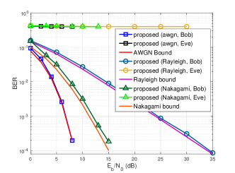
VII-E BER performance for Alice-Bob and Alice-Eve

Fig 10 demonstrates the BER performance of Alice-Bob and Alice-Eve links. As can be seen, the Alice-Bob link can achieve nearly the same BER performance as that in the ISI-free AWGN channel. For the Alice-Eve link, when $\alpha_{E}\neq\alpha_{A}$ , it will not be able to sample the received signals by the expected interval. Despite the assumption that when $\alpha_{E}=\alpha_{A}$ , sampling offset is not taken into consideration, the average BER of the Alice-Eve link is still poor enough.

VII-F The Power of Random Segment Starting Positions to Avoid Attack and Detection

Eve’s estimations on the exampled frame with sample-based and range-based sliding windows (presented in Fig. 11) are demonstrated in Fig. 12LABEL:sub@fig:result_new_c1 and Fig. 12LABEL:sub@fig:result_old_c1, respectively. An up-sampling with 20 times is employed. And the frame is constructed with $\alpha=0.9,0.8,0.7,0.6$ , where $\alpha$ for each segment has been marked in the figures.

The estimation in Fig. 12LABEL:sub@fig:result_new_c1 is based on $\eta_{1}$ continuous decisions with fixed interval $\alpha T_{N}$ , where $\eta_{1}$ is the length of the sliding window. As shown, the result is messy and it is difficult to find a pattern to map the estimation to the original packing ratio for each segment. In fact, the information of starting positions helps the receiver carry out the estimation at the perfect times to eliminate the interference of other erroneous results.

Another way for Eve’s estimation is to employ the continuous $\eta_{2}$ decisions with fixed interval $\alpha T_{N}/U_{s}$ , where $U_{s}$ is the up-sampling times. As shown in Fig. 12LABEL:sub@fig:result_old_c1, the estimation is still confusing. And especially, the starting position cannot be inferred by the estimation results.

VII-G BER Degradation of VPR-based Secure Transmission

According to the simulation results, the VPR-based secure transmission performs nearly the same SE with FTN signaling where $\alpha=0.8$ , $\beta=0.5$ and $\alpha=0.9$ , $\beta=0.3$ . So, we compare the BER of them under such two cases, where the following channel codings are considered.

•

Low density parity check (LDPC) code. We employ the (1296, 648) LDPC code with a rate of 1/2. The parity matrix is defined in [49]. And the back propagation (BP) is employed as the decoding algorithm.
•

Turbo code. We employ the (6298, 1256) Turbo code with a rate of 628/3149 and the constraint length of 4. The parity bits are obtained by $y_{1}=x^{3}+x^{1}+x^{0}$ and $y_{2}=x^{3}+x^{2}+x^{1}+x^{0}$ , where $x^{\kappa}$ represents the $\kappa$ -th bits in the state of shift registers. And the feedback bit is calculated by $r_{b}=x^{3}+x^{2}+x^{0}$ . The MAP is applied as the decoding algorithm.
•

Convolutional code (CC). We employ the (3768, 1256) CC with a rate of 1/3. The constraint length and the structure of the shift registers are the same as that of the turbo code presented in the previous item. No tail bits are required in this case. And Viterbi decoding with hard decisions is employed as the decoding algorithm.

The simulation results are demonstrated by Fig. 13LABEL:sub@fig:ber_0p5_c1 and Fig. 13LABEL:sub@fig:ber_0p3_c1.

As seen, with the same SE, the proposed VPR-based secure transmission can achieve nearly the same BER performance as the conventional FTN signaling. It means that the proposed scheme can achieve security at the expense of negligible BER performance degradation.

VII-H Comparison Between the Simplified Packing Ratio Estimation and the Original Architecture

In this part, we compare the simplified packing ratio estimation and its original architecture [38] by the complexity and the accuracy. For the convenience of representation, we only provide the complexity of the branch for analysis on $\alpha=0.7$ , while the total complexity is approximately proportional to it. Table III provides the complexity comparison between these two schemes.

TABLE III: The complexity comparison between the proposed simplified estimation and its original structure.

Algorithm	MUX	DEMUX	sum	max	S/P	$\lVert\mathbf{W}_{1}\rVert_{0}$	$\lVert\mathbf{W}_{2}\rVert_{0}$	$\lVert\mathbf{W}_{3}\rVert_{0}$	$\lVert\mathbf{W}_{4}\rVert_{0}$	multi-add
Original Structure	1	2	$10$	1	$10$	20k	500k	250k	0.25k	645.25k
Proposed Structure	0	0	1	0	1	10k	250k	62.5K	0.125k	about 32.263k

The proposed structure nearly removes all the MUX, DEMUX, sum, maximum and S/P operations in the original design. Also, in the sparse DNN employed in our proposed simplified estimation, the number of non-zero weights in each layer has been reduced to half of that in the original network. Significantly, benefiting from the sparse DNN and the single branch structure, the number of multiply-add operations required for each estimation has been reduced to 5% of that in the original architecture. This allows more flexibility for researchers to balance the resource of time and space in practical implementation.

To more visually demonstrate the performance, we employ the accuracy as [38]

\begin{split}P_{\mathrm{acc}}&=\sum_{m=1}^{M}\sum_{n=0}^{m-1}\left(C_{M}^{m}C_{M}^{n}\left(p_{1}\right)^{m}\left(1-p_{1}\right)^{(M-m)}\left(p_{2}\right)^{n}\left(1-p_{2}\right)^{(M-n)}\right)\end{split},

(79)

where $M$ is the number of decisions applied to determine the final estimated value of $\alpha$ . $p_{1}$ is the probability that the analysis branch for $\alpha_{k}=\alpha$ outputs integer $1$ (i.e., the diagonal items in Fig. 8). And $p_{2}$ is the maximum probabilities that the analysis branches for $\alpha_{k}\neq\alpha$ produce integer $1$ (i.e. the maximum one of non-diagonal items within each row in Fig. 8).

Fig. 14 shows the minimum number of decisions required to achieve a 99% accuracy ( $P_{acc}>0.99$ ). As seen, the proposed simplified estimation can converge nearly as fast as the original structure within 35 decisions, while the complexity has been greatly reduced.

VII-I Complexity of the Simplified Estimation and Other Common DL Networks

Here, two common deep learning networks named Transformer [50] and Inception-v4 [51] are considered for the comparison of complexity. They are both proposed by Google and have been widely employed in natural language processing (NLP) and computer vision (CV) research fields. Their effectiveness and complexity have been verified by mass researchers and applications.

The complexity comparison is shown in Table IV. As seen, the proposed scheme has an obviously lower complexity than the selected widely employed networks.

VII-J The Robustness of the Simplified Estimation to SNR Values

Here, the performance of the proposed simplified estimation for $\alpha=0.9$ in AWGN channels under different SNR values is listed in Table V. As shown, although the model is trained at SNR=4dB, it can work well for other SNR values. It can effectively reduce the resource required for the proposed estimation during both the training and the implementation stages.

TABLE IV: Complexity comparison between the proposed scheme and some common networks.

Network	Proposed	Transformer (base)	Transformer (big)	Resnet
Parameters	0.645M	65M	213M	48M
FLOPs	$6.5\times 10^{4}$	$3.3\times 10^{18}$	$2.3\times 10^{19}$	$1.3\times 10^{10}$

TABLE V: Performance of the proposed estimation which is trained at SNR=4dB and tested for different SNRs.

SNR	4dB	3dB	2dB	1dB
$p_{1}$	0.7534	0.5084	0.4372	0.2914
$p_{2}$	0.1632	0.1596	0.1463	0.1485
$M_{0.99}$	8	21	28	95
$M_{0.999}$	13	35	47	163

VIII Conclusion

This paper proposed intelligent VPR transmissions for high SE and security, respectively, based on FTN and DL. The VPR-based system achieved a higher SE without consuming extra spectrum resources and modifying the existing communication paradigms (e.g., spectrum allocation or frame structure). Also, considering security, a dynamic generation scheme was proposed to produce secret and randomly distributed positions for the segments of the VPR system. The scheme was demonstrated to be effective in avoiding detection and attack. In addition, we derived the closed-form expression for the capacity of the proposed VPR system in different channels, which were also effective for conventional FTN signaling. Finally, a simplified symbol packing ratio, which had been employed in the proposed system, was developed in this paper. Simulation results proved that it achieved nearly the same performance as the original structure with only 5% of the complexity in the original design.

In fact, there are still many open issues with the proposed VPR system beckoning further research. For example, how to design an effective switching strategy for the VPR system considering practical factors (e.g., interference, relay, energy harvesting, etc.), especially the nondeterministic polynomial (NP)-hard scenario is considered? How to derive the closed-form SE of the proposed scheme in other channels? Is it possible to develop a better packing ratio estimation algorithm to further improve the robustness of the VPR system? These issues will be studied in our future works.

References

[1] J. E. Mazo, “Faster-than-Nyquist signaling,” Bell Syst. Technical J., vol. 54, no. 8, pp. 1451–1462, 1975.
[2] A. D. Liveris and C. N. Georghiades, “Exploiting faster-than-Nyquist signaling,” IEEE Trans. Commun., vol. 51, no. 9, pp. 1502–1511, 2003.
[3] J. B. Anderson, A. Prlja, and F. Rusek, “New reduced state space BCJR algorithms for the ISI channel,” in Proc. IEEE Int. Symp. Inf. Theory, Seoul, South Korea. IEEE, 2009, pp. 889–893.
[4] E. Bedeer, M. H. Ahmed, and H. Yanikomeroglu, “A very low complexity successive symbol-by-symbol sequence estimator for faster-than-Nyquist signaling,” IEEE Access, vol. 5, no. 99, pp. 7414–7422, 2017.
[5] P. Song, F. Gong, Q. Li, G. Li, and H. Ding, “Receiver design for faster-than-Nyquist signaling: Deep-learning-based architectures,” IEEE Access, vol. 8, pp. 68 866–68 873, 2020.
[6] B. Liu, S. Li, Y. Xie, and J. Yuan, “A novel sum-product detection algorithm for faster-than-nyquist signaling: A deep learning approach,” IEEE Trans. Commun., vol. 69, no. 9, pp. 5975–5987, 2021.
[7] T. Petitpied, R. Tajan, P. Chevalier, S. Traverso, and G. Ferré, “Circular faster-than-Nyquist signaling for high spectral efficiencies: optimized EP-based receivers,” IEEE Trans. Commun., vol. 69, no. 8, pp. 5487–5501, 2021.
[8] A. Ibrahim, E. Bedeer, and H. Yanikomeroglu, “A novel low complexity faster-than-nyquist signaling detector based on the primal-dual predictor-corrector interior point method,” IEEE Commun. Lett., vol. 25, no. 7, pp. 2370–2374, 2021.
[9] S. Sugiura, “Frequency-domain equalization of faster-than-Nyquist signaling,” IEEE Wireless Commun. Lett., vol. 2, no. 5, pp. 555–558, 2013.
[10] T. Ishihara and S. Sugiura, “Frequency-domain equalization aided iterative detection of faster-than-Nyquist signaling with noise whitening,” in Proc. IEEE Int. Conf. Commun. (ICC), Kuala Lumpur, Malaysia. IEEE, 2016, pp. 1–6.
[11] F. Rusek and J. B. Anderson, “Multistream faster than nyquist signaling,” IEEE Trans. Commun., vol. 57, no. 5, pp. 1329–1340, 2009.
[12] H. Che, K. Zhu, and Y. Bai, “Multicarrier faster-than-Nyquist based on efficient implementation and probabilistic shaping,” IEEE Access, vol. 9, pp. 63 943–63 951, 2021.
[13] T. Ishihara and S. Sugiura, “Reduced-complexity FFT-spread multi-carrier faster-than-Nyquist signaling in frequency-selective fading channel,” IEEE Open J. Commun. Soc., 2022.
[14] Y. Ma, N. Wu, A. Zhang, B. Li, and L. Hanzo, “Generalized approximated message passing equalization for multi-carrier faster-than-Nyquist signaling,” IEEE Trans. Veh. Technol., 2021.
[15] J. B. Anderson and F. Rusek, “Improving OFDM: Multistream faster-than-Nyquist signaling,” in proc, 4th Int. Symp. Turbo Codes & Related Topics; 6th Int. ITG-Conference on Source and Channel Coding. VDE, 2006, pp. 1–5.
[16] F. Rusek, “On the existence of the Mazo-limit on MIMO channels,” IEEE Trans. Wireless Commun., vol. 8, no. 3, pp. 1118–1121, 2009.
[17] A. T. Abebe and C. G. Kang, “FTN-based MIMO transmission as a NOMA scheme for efficient coexistence of broadband and sporadic traffics,” in proc, 2018 IEEE 87th Veh. Technol. Conf. (VTC Spring). IEEE, 2018, pp. 1–5.
[18] M. Yuhas, Y. Feng, and J. Bajcsy, “On the capacity of faster-than-Nyquist MIMO transmission with CSI at the receiver,” in proc, 2015 IEEE Globecom Workshops (GC Wkshps). IEEE, 2015, pp. 1–6.
[19] M. McGuire, A. Dimopoulos, and M. Sima, “Faster-than-Nyquist single-carrier MIMO signaling,” in proc, 2016 IEEE Globecom Workshops (GC Wkshps). IEEE, 2016, pp. 1–7.
[20] S. Wen, G. Liu, C. Liu, H. Qu, L. Zhang, and M. A. Imran, “Joint precoding and pre-equalization for faster-Than-Nyquist transmission over multipath fading channels,” IEEE Trans. Veh. Technol., 2022.
[21] T. Ishihara and S. Sugiura, “Iterative frequency-domain joint channel estimation and data detection of faster-than-Nyquist signaling,” IEEE Trans. Wireless Commun., vol. 16, no. 9, pp. 6221–6231, 2017.
[22] Q. Li, F.-K. Gong, P.-Y. Song, G. Li, and S.-H. Zhai, “Joint channel estimation and precoding for faster-than-Nyquist signaling,” IEEE Trans. Veh. Technol., vol. 69, no. 11, pp. 13 139–13 147, 2020.
[23] T. Ishihara, S. Sugiura, and L. Hanzo, “The evolution of faster-than-Nyquist signaling,” IEEE Access, vol. 9, 2021.
[24] J. Zhou, M. Guo, Y. Qiao, H. Wang, L. Liu et al., “Digital signal processing for faster-than-Nyquist non-orthogonal systems: An overview,” in proc, 2019 26th Int. Conf. Telecommun. (ICT). IEEE, 2019, pp. 295–299.
[25] J. Fan, S. Guo, X. Zhou, Y. Ren, G. Y. Li, and X. Chen, “Faster-than-Nyquist signaling: an overview,” IEEE Access, vol. 5, pp. 1925–1940, 2017.
[26] F. Rusek and J. B. Anderson, “Constrained capacities for faster-than-Nyquist signaling,” IEEE Trans. Inf. Theory, vol. 55, no. 2, pp. 764–775, 2009.
[27] J. Wang, W. Tang, X. Li, and S. Li, “Filter hopping based faster-than-Nyquist signaling for physical layer security,” IEEE Wireless Commun. Lett., vol. 64, no. 5, pp. 2122–2128, 2018.
[28] ETSI, “Digital video broadcasting (DVB); implementation guidelines for the second generation system for broadcasting, interactive services, news gathering and other broadband satellite applications; part 1: DVB-S2,” available: https://www.etsi.org/deliver/etsi_tr/102300_102399/10237601/01.02.01_60/tr_10237601v010201p.pdf, 2015.
[29] T. Aono, K. Higuchi, T. Ohira, B. Komiyama, and H. Sasaoka, “Wireless secret key generation exploiting reactance-domain scalar response of multipath fading channels,” IEEE Trans. Antennas Propag., vol. 53, no. 11, pp. 3776–3784, 2005.
[30] S. Mathur, W. Trappe, N. Mandayam, C. Ye, and A. Reznik, “Radio-telepathy: extracting a secret key from an unauthenticated wireless channel,” in Proceedings of the 14th ACM international conference on Mobile computing and networking, 2008, pp. 128–139.
[31] N. Patwari, J. Croft, S. Jana, and S. K. Kasera, “High-rate uncorrelated bit extraction for shared secret key generation from channel measurements,” IEEE Trans. Mob. Comput., vol. 9, no. 1, pp. 17–30, 2009.
[32] G. Brassard and L. Salvail, “Secret-key reconciliation by public discussion,” in proc, Workshop on the Theory and Application of of Cryptographic Techniques. Springer, 1993, pp. 410–423.
[33] A. Rukhin, J. Soto, J. Nechvatal, M. Smid, and E. Barker, “A statistical test suite for random and pseudorandom number generators for cryptographic applications,” Booz-allen and hamilton inc mclean va, Tech. Rep., 2001.
[34] M. G. Madiseh, S. W. Neville et al., “Applying beamforming to address temporal correlation in wireless channel characterization-based secret key generation,” IEEE Trans. Inf. Forensics Secur., vol. 7, no. 4, pp. 1278–1287, 2012.
[35] N. Aldaghri and H. Mahdavifar, “Physical layer secret key generation in static environments,” IEEE Trans. Inf. Forensics Secur., vol. 15, pp. 2692–2705, 2020.
[36] A. Sayeed and A. Perrig, “Secure wireless communications: Secret keys through multipath,” in proc, 2008 IEEE International Conference on Acoustics, Speech and Signal Processing. IEEE, 2008, pp. 3013–3016.
[37] I. Goodfellow, Y. Bengio, and A. Courville, Deep Learning. MIT press, 2016.
[38] P. Song, F. Gong, and Q. Li, “Blind symbol packing ratio estimation for faster-than-nyquist signalling based on deep learning,” Electron. Lett., vol. 55, no. 21, pp. 1155–1157, 2019.
[39] S. O. Rice, “Mathematical analysis of random noise,” Bell Syst. Technical J., vol. 23, no. 3, pp. 282–332, 1944.
[40] M. Nakagami, “The m-distribution-a general formula of intensity distribution of rapid fading,” Statal Methods in Radio Wave Propagation, pp. 3–6, 1960.
[41] E. Cubukcu, “Root raised cosine (rrc) filters and pulse shaping in communication systems,” in proc, AIAA Conference, no. JSC-CN-26387, 2012.
[42] M. Abramowitz and I. A. Stegun, Handbook of mathematical functions with formulas, graphs, and mathematical tables. US Government printing office, 1964, vol. 55.
[43] G. B. Thomas and R. L. Finney, Calculus. Addison-Wesley Publishing Company, 1961.
[44] C. C. Ross, Differential equations: an introduction with Mathematica. Springer Science & Business Media, 2004.
[45] P. Flajolet, X. Gourdon, and P. Dumas, “Mellin transforms and asymptotics: Harmonic sums,” Theoretical Comput. Sci., vol. 144, no. 1-2, pp. 3–58, 1995.
[46] S. Edition, “Table of integrals, series, and products,” 2007.
[47] H. Bateman, Higher transcendental functions [volumes i-iii]. McGraw-Hill Book Company, 1953, vol. 1.
[48] S. Li, B. Bai, J. Zhou, P. Chen, and Z. Yu, “Reduced-complexity equalization for faster-than-Nyquist signaling: New methods based on Ungerboeck observation model,” IEEE Trans. Commun., vol. 66, no. 3, pp. 1190–1204, 2018.
[49] “IEEE standard for information technology–telecommunications and information exchange between systems - local and metropolitan area networks–specific requirements - part 11: Wireless lan medium access control (MAC) and physical layer (PHY) specifications - redline,” IEEE Std 802.11-2020 (Revision of IEEE Std 802.11-2016) - Redline, pp. 1–7524, 2021.
[50] A. Vaswani, N. Shazeer, N. Parmar, J. Uszkoreit, L. Jones, A. N. Gomez, Ł. Kaiser, and I. Polosukhin, “Attention is all you need,” Advances in neural information processing systems, vol. 30, 2017.
[51] C. Szegedy, S. Ioffe, V. Vanhoucke, and A. A. Alemi, “Inception-v4, inception-resnet and the impact of residual connections on learning,” in proc, Thirty-first AAAI conference on artificial intelligence, 2017.