Forecasts for Helium Reionization Detection with Fast Radio Bursts in the Era of Square Kilometre Array
Abstract
The observed dispersion measures (DMs) of fast radio bursts (FRBs) are a good indicator of the amount of ionized material along the propagation paths. In this work, we present a forecast of He ii reionization detection using the DM and redshift measurements of FRBs from the upcoming Square Kilometre Array (SKA). Assuming a model of the Universe in which He ii reionization occurred at a specific redshift , we analyze what extent the signal-to-noise ratio () for the detection of the amplitude of reionization can be achieved in the era of SKA. Using mock FRB data from a one-year observation of the second phase of SKA, we find that the for detecting He ii reionization can approach the level and the uncertainty on the reionization redshift can be constrained to be , depending on the assumed FRB redshift distribution. This is the first quantitative analysis on the detection significance of He ii reionization in the SKA era. We also examine the influence of different fiducial values, finding that this effect has a modest impact on the forecasts. Our results demonstrate the potentially remarkable capability of SKA-era FRBs in constraining the epoch of He ii reionization.
1 Introduction
Reionization is regarded as the latest phase transition in the Universe, transforming the baryonic gas from a neutral condition into an ionized state (Barkana & Loeb, 2001). Understanding how and when the cosmic reionization happened is one of the important research topics in modern cosmology. Reionization usually refers to the process by which neutral hydrogen and helium atoms lost their first outer electrons at redshifts (e.g., Fan et al. 2002; Zaroubi 2013; Singh et al. 2018). During the epoch of hydrogen reionization, the high ionization potential () of singly ionized helium (He ii) kept its inner electron from being further ionized. The reionization of He ii, caused by sufficient strong radiation from quasars and stars, is generally believed to occur at . The strongest evidence of He ii reionization is obtained from observational signatures of the He ii Ly forest in the spectra of quasars at (Syphers et al., 2009, 2012; Basu et al., 2024). Other evidence is the temperature change of the intergalactic medium (IGM; Furlanetto & Oh 2008a, b; McQuinn et al. 2009). The relatively lower redshift of He ii reionization enables it more likely to be detected by next generation surveys.
Fast radio bursts (FRBs) are bright millisecond radio pulses predominantly originate at cosmological distances, the study of which is a hot spot in contemporary astrophysics (Lorimer et al., 2007; Cordes & Chatterjee, 2019; Petroff et al., 2019, 2022; Xiao et al., 2021; Zhang, 2023). Their all-sky rate is estimated to be as high as (Thornton et al., 2013). A direct observable of FRBs is the dispersion measure (DM) that encodes the integrated column density of ionized plasma along the line of sight. The observed DM is thus a good indicator of the amount of ionized baryons along the propagation path between the FRB source and the observer. Moreover, some FRBs with extremely high DM measurements are expected to be detected up to by future large-aperture telescopes (Fialkov & Loeb, 2017; Zhang, 2018; Hashimoto et al., 2020). Thanks to the short pulse nature, the high event rate, and the cosmological origin, FRBs are suitable for being used as a potentially new probe for the ionized IGM. Several studies have proposed that future DM measurements of high- FRBs could be used to constrain the reionization history of hydrogen (e.g., Deng & Zhang 2014; Beniamini et al. 2021; Dai & Xia 2021; Hashimoto et al. 2021; Pagano & Fronenberg 2021; Heimersheim et al. 2022; Maity 2024; Shaw et al. 2024) and helium (e.g., Deng & Zhang 2014; Zheng et al. 2014; Caleb et al. 2019; Linder 2020; Bhattacharya et al. 2021; Lau et al. 2021; Jing & Xia 2022). Since the current sample size and redshift range of localized FRBs are small, all such studies were performed by building mock FRB data sets.
As a next-generation radio astronomy-driven Big Data facility (Macquart et al., 2015), the Square Kilometre Array (SKA) will definitely have very powerful capability of detecting and localizing high- FRBs (Fialkov & Loeb, 2017; Hashimoto et al., 2020), which will offer a much larger population of FRBs for exploring the epoch of reionization. Therefore, it is natural to ask what level of reionization constraints can be achieved using future FRB data in the era of SKA. In view of the fact that He ii reionization happened at a comparatively lower redshift and is more accessible to measurements, here we investigate the ability of the SKA-era FRB observation to detect He ii reionization through Monte Carlo simulations.
But though FRBs have previously been proposed to constrain the epoch of He ii reionization (Deng & Zhang, 2014; Zheng et al., 2014; Caleb et al., 2019; Linder, 2020; Bhattacharya et al., 2021; Lau et al., 2021; Jing & Xia, 2022), it has not yet been quantitatively analyzed what extent the nature of He ii reionization can be explored in the SKA era—our primary focus in this paper. Previously, Deng & Zhang (2014) and Zheng et al. (2014) first proposed the potential application of FRBs in probing He ii reionization, Caleb et al. (2019) estimated the number of FRBs required to distinguish between a sudden He ii reionization that occurred at or by using a two-sample Kolmogorov-Smirnoff test, Linder (2020) assessed the ability of future high- FRB samples to detect He ii reionization, Bhattacharya et al. (2021) showed that the statistical ensemble of the DM distribution of FRBs prove useful probes of He ii reionization even with limited redshift information, Lau et al. (2021) presented a cosmology-based model on determining the He ii reionization redshift in range of to by detecting the DMs of distant FRBs, and Jing & Xia (2022) attempted to use the DM– measurements of FRBs to derive the helium abundance in the Universe. In this work, we build on the techniques outlined by these authors by performing a forecast of the detection significance of He ii reionization with the SKA-era FRB observation.
The rest of this paper is organized as follows. In Section 2, we show the imprint of the occurrence of He ii reionization on the redshift function of the IGM portion of the DM, i.e., , and describe the definition of a signal-to-noise ratio () for the detection of He ii reionization. The expected detection rates of FRBs by SKA, the simulation method, and the relevant analysis results are presented in Section 3. Finally, we give a brief summary and discussion in Section 4. Throughout this paper, we assume CDM cosmology and adopt the cosmological parameters of km , , , and (Planck Collaboration et al., 2020).
2 Impact of Helium Reionization on Dispersion Measure
For an extragalactic FRB propagating through the IGM, the cosmic DM in the observer frame is related to the free electron density () along the line of sight:
| (1) |
In a flat CDM cosmology, the relation between proper length element and redshift is given by
| (2) |
where is the speed of light, is the Hubble constant, is the present-day matter density, and is the vacuum energy density. The number density of free electrons can be expressed as (Deng & Zhang, 2014)
| (3) |
where is the critical density of the Universe, is the proton mass, is the baryon density parameter, and is the mass fraction of baryons in the IGM (Fukugita et al., 1998). The electron fraction is
| (4) |
where and are the hydrogen and helium abundances in the Universe, respectively, and and represent the ionization mass fractions of hydrogen and helium, respectively. The singly and doubly ionized elements are denoted by subscripts “II” and “III”, respectively. At a given redshift, the measured value of would vary along different lines of sight due to the large density fluctuations in IGM. In theory, the averaged over different lines of sight can be estimated by (Ioka, 2003; Inoue, 2004)
| (5) |
At the epoch of hydrogen reionization, both neutral hydrogen and helium are singly ionized by ionizing photons emitted from star-forming galaxies, can thus be approximated as (e.g., Dai & Xia 2021). We suppose that hydrogen is fully ionized at (i.e., and ) and that He ii reionization occurs suddenly at redshift (i.e., and ). That is, considering the FRB sample up to redshifts , one has , , and before He ii reionization, while afterward , , and . Thus, and , where we adopt the helium abundance inferred from Planck observations: (Planck Collaboration et al., 2020). The ionization fraction increases by because of He ii reionization. That is, the sudden He ii reionization would cause a change in (Equation 5).
It is interesting to explore whether we can detect such He ii reionization in the DM– measurements of a high- FRB sample. Following Linder (2020), we define a simple criterion for the detection of He ii reionization. In practice, we model the detection as (Linder, 2020)
| (6) |
where the superscripts “high” and “” mean He ii reionization occurs beyond the redshift limit of the sample and at , respectively. If , then He ii reionization is not detected by the sample, while corresponds to reionization occurring at . With representing the uncertainty of the determined , the detection is thus , or simply since it gives if the modeling is right.
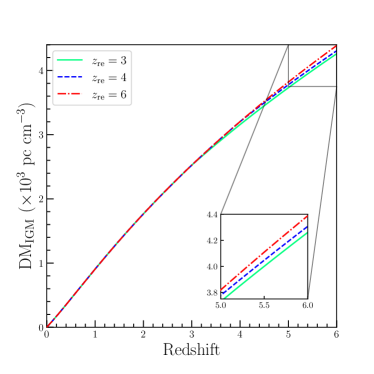
As an illustration, the DM of the IGM as a function of the redshift is given in Figure 1. To show the effect of a sharp He ii reionization on , we plot three cases with reionization occurring at and , respectively. It is obvious that the cosmic DM has a change in slope at the reionization redshift due to the extra influx of electron fraction from He ii reionization. The key questions are thus whether this signature (i.e., identify with significant ) can be detected, and whether the redshift at which reionization occurs can be measured. The model curves look pretty close together, as shown in Figure 1, but it should be underlined that the for the detection of He ii reionization would be enhanced by having enough high- FRBs on either side of the reionization redshift. In the next section, we will investigate the prospect of He ii reionization detection with the SKA-era FRB observation.
3 Forecasting with FRB mock
3.1 Detection Rate of FRBs in the SKA era
Thanks to their extremely high event rate (Thornton et al., 2013), abundant FRBs are expected to be detected by the upcoming telescopes. Note that uncertainties in the fluence distribution and spectral index of the FRB population would make the estimate of the event detection rate for a specific telescope uncertain by several orders of magnitude (Vedantham et al., 2016; James et al., 2019; Zhang et al., 2023). However, it is feasible to give a simple calculation on the event detection rate at operating frequencies close to those at which FRB detections are conducted (i.e., 1.2–1.7 GHz, as probed by the SKA’s mid-frequency instrument), based on reasonable assumptions on the slope of the differential fluence distribution (i.e., the distribution). The cumulative all-sky event rate of FRBs above a given fluence threshold is generally described as a power-law model (Macquart & Ekers, 2018),
| (7) |
where is the known event rate above the fluence threshold estimated by existing FRB surveys, and the power-law index is in line with the expectation of a non-evolving population in Euclidean space (Vedantham et al., 2016).
The mid-frequency aperture array of the first phase of SKA (SKA1-MID) would reach a sensitivity of from 0.9 to 1.67 for an integration time of 1 ms (Fender et al., 2015). While the actual scope of the second phase of SKA (SKA2) will eventually be subject to further discussions, the performance of SKA2 may be 10 times the SKA1 sensitivity in the frequency range of 0.35–24 .111https://www.skao.int/en/science-users/118/ska-telescope-specifications That is, the adopted fluence threshold of SKA2-MID is . With Equation (7), we can estimate the all-sky event rate observed by SKA2-MID based on the rate measurements of Parkes and ASKAP telescopes. Bhandari et al. (2018) obtained above the fluence threshold of from Parkes FRB surveys. Shannon et al. (2018) obtained above the fluence threshold of from ASKAP FRB surveys. Based on the Parkes result, the estimated all-sky event rate for SKA2-MID is
| (8) |
and according to the ASKAP result, we have
| (9) |
It is obvious that the two estimates are in good agreement with each other.
Considering the solid angle covered on the sky by the SKA instantaneous observation, the expected number of FRBs can be estimated by
| (10) |
where is the exposure time on source. In general, the overall sky coverage of SKA2-MID would reach (Torchinsky et al., 2016). Since FRBs are transient phenomena, here we conservatively take as the effective instantaneous field of view of SKA2-MID (Macquart et al., 2010). Following Zhang et al. (2023), we assume that SKA2-MID would spend an average of 20% of observing time per year on FRB search, and take . On the basis of the Parkes and ASKAP results, the expected detection rates of FRBs by SKA2-MID are then and , respectively. Thus, we conclude that FRBs can be detected by SKA2-MID in a one-year observation.
The precise localization of FRBs is crucial for FRB cosmology. To obtain their host galaxy redshifts via optical follow-up, the positions of FRBs should be localized to within one arcsecond (Macquart et al., 2015). When complete, the SKA will have the ability of localizing FRBs to an accuracy of sub-arcseconds, and thus it is reasonable to expect that all the host galaxies of the SKA-detected FRBs would be identified and their redshifts would be measured.
3.2 Mock FRB Data
In this work, we perform Monte Carlo simulations to explore the prospect of He ii reionization detection with future FRB measurements in the SKA era. The fiducial flat CDM model with cosmological parameters derived from Planck observations ( km , , and ; Planck Collaboration et al. 2020) is adopted to simulate FRB data. The fiducial values of the reionization parameters are taken to be and , though we will discuss the effect of different fiducial in the following subsection.
The redshift distribution of FRBs is expressed as
| (11) |
where is the comoving distance, is the Hubble parameter, and denotes the intrinsic event rate density distribution. So far, the actual distribution of FRBs is poorly known. Qiang & Wei (2021) stressed that the assumed redshift distributions (i.e., the assumed distributions) have significant effect on cosmological parameter estimation. The true redshift distribution of FRBs is inextricably linked to the corresponding progenitor system(s) of FRBs, and it is commonly assumed that the FRB rate follows the cosmic star formation history (SFH) or compact star mergers. In the merger model, a compact star binary system needs to experience a long inspiral phase before the final merger, so there is a significant time delay with respect to star formation. In the literature, three types of merger delay timescale models have been discussed (Virgili et al., 2011; Sun et al., 2015; Wanderman & Piran, 2015): Gaussian delay model, lognormal delay model, and power-law delay model. Thus, we investigate four FRB event rate density models in detail:
-
•
SFH model: we adopt the approximate analytical form derived by Yüksel et al. (2008) using a wide range of the star formation rate data
(12) where .
-
•
Compact star merger models: for the Gaussian delay model, we adopt the empirical formula (Virgili et al., 2011)
(13) where .
-
•
Compact star merger models: for the lognormal delay model (Wanderman & Piran, 2015), the empirical formula of is
(14) where .
-
•
Compact star merger models: for the power-law delay model (Wanderman & Piran, 2015), one has
(15) where .
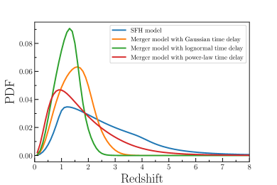
Figure 2 presents the FRB redshift distributions expected from all four assumed models. It is clear that the SFH model has the widest distribution. Due to the merger delay, the other three merger models have narrower distributions, with the overall redshift gradually shifting to lower redshifts in the order of power-law, Gaussian, and lognormal models (Zhang et al., 2021). Note that He ii reionization is generally expected to occur at (e.g., Becker et al. 2011). In order to effectively detect the signature of He ii reionization, many high- FRBs on either side of the expected reionization redshift are required. However, only low- () FRBs are predicted by the Gaussian and lognormal delay models (see Figure 2). For the rest of this paper, we shall therefore only consider two cases: the FRB redshift distribution tracing the SFH and power-law delay models, respectively.
In our simulations, the true FRB host galaxy redshifts are randomly generated from the probability density functions (PDFs) of Equation (11) for the SFH and power-law delay cases. After generating , we simulate the measured redshifts by assuming an uncertainty of 10% on the spectroscopic data of host galaxies (as expected from the James Webb Space Telescope). That is, we draw from a Gaussian distribution (Heimersheim et al., 2022; Maity, 2024).
With the true source redshift , we infer the fiducial value of from Equation (6). Following previous works (Kumar & Linder, 2019; Linder, 2020), the line-of-sight fluctuation of () is randomly added to the fiducial value of , assuming
| (16) |
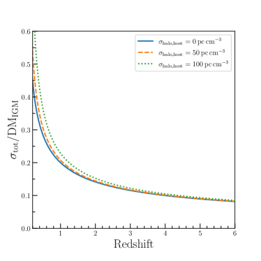
That is, we sample the measurement according to the Gaussian distribution . We note that the observed has contributions from the interstellar medium () and dark matter halo () in the Milky Way, the IGM (), and the FRB host galaxy (). The value can then be derived by deducting , , and to . While the corresponding uncertainty of should include the scatter due to the inhomogeneous IGM and the scatter caused by distinctive host properties and halo, the latter scatter (order of ) is much smaller than the former one (order of ) at the reionization epoch (e.g., Prochaska & Zheng 2019). Figure 3 shows the evolution of the fractional uncertainty on a measured , accounting for the line-of-sight fluctuation of () and the uncertainty of both and (), i.e., . At low redshift, is small, so the fractional uncertainty is relatively large. Since lines of sight average over IGM inhomogeneity and increases at higher redshift, gradually decreases. Moreover, one can see from Figure 3 that adding the halo and host uncertainty (with the value of or ) in quadrature gives negligible effect on , especially around the expected reionization redshift . Therefore, we neglect the uncertainty of both and subtractions from to derive observationally.
Using the method described above, one can generate a catalog of the simulated FRB events with , , and . Due to the lack of computational efficiency, we first simulate a population of such events, assuming that the FRB redshift distribution follows the SFH model or the power-law delay model separately.
3.3 Results
For a set of simulated FRBs, we only employ those FRBs with for He ii reionization parameter estimation, since the ionization fractions of hydrogen at are not well understood and we take all of the hydrogen to be ionized at . We then utilize the standard Bayes theorem to explore the posterior probability distribution of the model parameters , provided the observed dataset , i.e.,
| (17) |
where is the likelihood of data conditional on the hypothetical model, denotes some prior knowledge about the model parameters, and is the Bayesian evidence (which can be regarded as the normalized parameter and has no effect on our analysis). In our study, is the mock dataset consisting of and , and the free parameters to be constrained are . The likelihood is given by (Maity, 2024)
| (18) |
where is the theoretical value of calculated from the set of He ii reionization parameters (see Equation 6). To ensure the final resulting constraints are unbiased, the simulation process is repeated 100 times for each FRB data set by using different noise seeds.
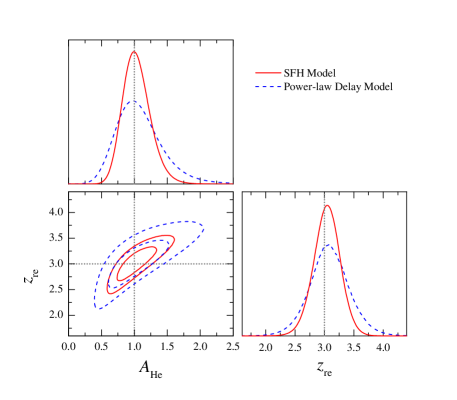
Figure 4 displays the resulting constraints on the reionization parameters and from simulated FRBs. For the case of distribution tracing the SFH model (solid contours), we find the marginalized parameter uncertainties are and . That is, the detection for He ii reionization is . Besides, the sudden reionization redshift can be inferred to be . To investigate the effect of distribution, in Figure 4 we also plot those constraints obtained from the case of distribution tracing the power-law delay model (dashed contours). Now we have and . The detection decreases to . We can see that the constraint precisions of and obtained from the power-law delay model are slightly worse than those from the SFH model. This is mainly because reionization parameters are more sensitive to high- FRB data, and more high- mock events, especially around the expected reionization redshift , are generated in the SFH model (see Figure 2).
| SFH Model | Power-law Delay Model | |||
|---|---|---|---|---|
| 1 | ||||
| 2 | ||||
| 3 | ||||
| 4 | ||||
| 5 | ||||
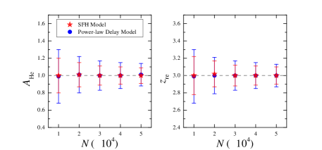
In order to comprehensively test what role the number of simulated FRBs () could play in He ii reionization detection, we show the best-fit reionization parameters and their corresponding uncertainties as a function of in Figure 5 and Table 1. We find that the uncertainties of these constraints from the FRB data are well consistent with the behavior, independent of what kind of distribution is assumed. According to our estimation of the FRB detection rate by SKA2-MID in Section 3.1, the one-year SKA2 observation would detect FRBs. In principle, it would be ideal to show the analysis with mock FRBs. However, due to the lack of computational efficiency, we estimate the capacity of mocks by extrapolating from present results of mocks. Since all uncertainties will scale in proportion to the behavior, FRB data can give the reionization parameter uncertainties and ( and ) for the case of distribution tracing the SFH (power-law delay) model. Hence, for a one-year SKA2 observation with FRBs, the detection can approach 32–50.
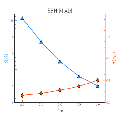
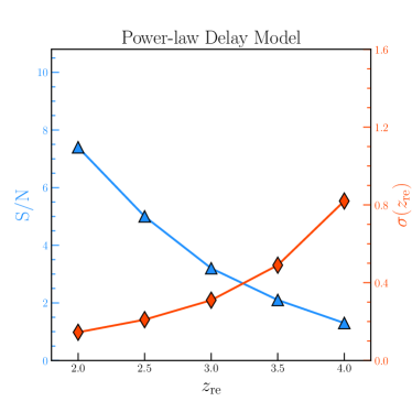
In our above simulations, the fiducial reionization redshift is set to be . To study the effect of different fiducial , we estimate the sensitivity as we vary . Note that here we also mock a population of FRBs with the distribution following the SFH and power-law delay models, respectively. Figure 6 shows that no matter which distribution is assumed, the gets better rapidly with lower , but falls below for . As the fiducial value of grows, the reionization redshift uncertainty becomes larger. These are pretty easy to understand, because the number of FRBs at higher is smaller (see the blue and red lines in Figure 2). Over the main range of the expected reionization redshifts, say , the varies from 7.4 (5.0) to 3.2 (2.1), and varies from 0.16 (0.21) to 0.29 (0.49) for the SFH (power-law delay) model.
In our analysis, we have neglected the uncertainty of the DM contributions from both the Milky Way halo and the FRB host (), as described in Section 3.2. Although it seems to be a reasonable treatment as suggested by Figure 3, it would be good to add an analysis incorporating and check if there is any bias in the posterior recovery. Especially, when He ii reionization is assumed to occur at , adding the halo and host uncertainty (for the maximum case of ) in quadrature gives a slight increasement of (see Figure 3). To investigate how sensitive our results on the uncertainties of and are on the choice of , we also perform two parallel comparative analyses of simulated FRBs using and , assuming that the fiducial reionization redshift is and the distribution traces the power-law delay model. If we change from to , then goes from to , and from to . So there is no concern regarding a possibly large dependence on .
We emphasize that all our results are based on the assumption of sudden He ii reionization. However, in reality, it is expected that the reionization phenomenon should evolve gradually with . Assuming a linear evolution in redshift for the He ii reionization within a range of to , Bhattacharya et al. (2021) found that the difference between results for sudden reionization and gradual reionization is generally not significant. This is a positive outcome in the sense that our results on He ii reionization detection are robust to the assumption about suddenness, but does imply that the duration of the reionization process is difficult to determine.
4 Summary and discussion
Cosmic reionization typically refers to the ionization of neutral hydrogen and helium at redshifts . The singly ionized helium, He ii, is expected to have undergone the same phase transition, but at a relatively lower redshift, and is often referred to as He ii reionization. Compared to the former one related to neutral hydrogen and helium reionization above , the later He ii reionization is more accessible to observations by next generation surveys. FRBs, with their short pulse nature, high event rate, and large cosmological distance, are a promising tool for probing the epoch of He ii reionization.
In this work, we have investigated the prospect of He ii reionization detection with future FRB data to be detected by the upcoming SKA. With the definition of a simple criterion for detecting He ii reionization, we performed Monte Carlo simulations to assess the ability of the SKA-era FRB observation to constrain the detection and the redshift at which reionization occurs. In our simulations, we considered two different FRB redshift distributions: one is assumed to follow the SFH model, and the other one traces the compact star merger model with power-law merger delay time distribution. Based on a mock catalog of FRBs, our results showed that the detection and the uncertainty of the reionization redshift , depending on the assumed distribution. Moreover, we confirmed that the uncertainties of the marginalized reionization parameters are in good agreement with the behavior, with the number of simulated FRBs. According to the existing FRB surveys and the possible detection performance of SKA2-MID, we expected that FRBs would be detected by SKA2 in a one-year observation. Since all the reionization parameter uncertainties will scale as , FRB data can give and . That is, for a one-year SKA2 observation with FRBs, the for the detection of He ii reionization can approach the level. We also inspected how the fiducial value of the reionization redshift affect the forecasts for He ii reionization detection, and found this effect was modest within the main range of the expected reionization redshifts.
It is worth highlighting that detecting high- FRBs is very important scientifically. After the completion of SKA, an extensive dataset of high- FRBs might become available. This would provide a great opportunity to utilize the DM measurements of high- FRBs to directly probe the state of reionization in the IGM. Moreover, other world-leading radio survey telescopes such as the Hydrogen Intensity and Real-time Analysis eXperiment (HIRAX; Newburgh et al. 2016), Deep Synoptic Array 2000-dishes (DAS-2000; Hallinan et al. 2019), and Canadian Hydrogen Observatory and Radio-transient Detector (CHORD; Vanderlinde et al. 2019) are also anticipated to detect and localize tens of thousands of FRBs. With the rapid development of FRB detections, revealing the history of He ii reionization with FRBs would be turned into reality.
References
- Barkana & Loeb (2001) Barkana, R., & Loeb, A. 2001, Phys. Rep., 349, 125, doi: 10.1016/S0370-1573(01)00019-9
- Basu et al. (2024) Basu, A., Garaldi, E., & Ciardi, B. 2024, MNRAS, 532, 841, doi: 10.1093/mnras/stae1488
- Becker et al. (2011) Becker, G. D., Bolton, J. S., Haehnelt, M. G., & Sargent, W. L. W. 2011, MNRAS, 410, 1096, doi: 10.1111/j.1365-2966.2010.17507.x
- Beniamini et al. (2021) Beniamini, P., Kumar, P., Ma, X., & Quataert, E. 2021, MNRAS, 502, 5134, doi: 10.1093/mnras/stab309
- Bhandari et al. (2018) Bhandari, S., Keane, E. F., Barr, E. D., et al. 2018, MNRAS, 475, 1427, doi: 10.1093/mnras/stx3074
- Bhattacharya et al. (2021) Bhattacharya, M., Kumar, P., & Linder, E. V. 2021, Phys. Rev. D, 103, 103526, doi: 10.1103/PhysRevD.103.103526
- Caleb et al. (2019) Caleb, M., Flynn, C., & Stappers, B. W. 2019, MNRAS, 485, 2281, doi: 10.1093/mnras/stz571
- Cordes & Chatterjee (2019) Cordes, J. M., & Chatterjee, S. 2019, ARA&A, 57, 417, doi: 10.1146/annurev-astro-091918-104501
- Dai & Xia (2021) Dai, J.-P., & Xia, J.-Q. 2021, J. Cosmology Astropart. Phys, 2021, 050, doi: 10.1088/1475-7516/2021/05/050
- Deng & Zhang (2014) Deng, W., & Zhang, B. 2014, ApJ, 783, L35, doi: 10.1088/2041-8205/783/2/L35
- Fan et al. (2002) Fan, X., Narayanan, V. K., Strauss, M. A., et al. 2002, AJ, 123, 1247, doi: 10.1086/339030
- Fender et al. (2015) Fender, R., Stewart, A., Macquart, J. P., et al. 2015, in Advancing Astrophysics with the Square Kilometre Array (AASKA14), 51, doi: 10.22323/1.215.0051
- Fialkov & Loeb (2017) Fialkov, A., & Loeb, A. 2017, ApJ, 846, L27, doi: 10.3847/2041-8213/aa8905
- Fukugita et al. (1998) Fukugita, M., Hogan, C. J., & Peebles, P. J. E. 1998, ApJ, 503, 518, doi: 10.1086/306025
- Furlanetto & Oh (2008a) Furlanetto, S. R., & Oh, S. P. 2008a, ApJ, 681, 1, doi: 10.1086/588546
- Furlanetto & Oh (2008b) —. 2008b, ApJ, 682, 14, doi: 10.1086/589613
- Hallinan et al. (2019) Hallinan, G., Ravi, V., Weinreb, S., et al. 2019, in Bulletin of the American Astronomical Society, Vol. 51, 255, doi: 10.48550/arXiv.1907.07648
- Hashimoto et al. (2020) Hashimoto, T., Goto, T., On, A. Y. L., et al. 2020, MNRAS, 497, 4107, doi: 10.1093/mnras/staa2238
- Hashimoto et al. (2021) Hashimoto, T., Goto, T., Lu, T.-Y., et al. 2021, MNRAS, 502, 2346, doi: 10.1093/mnras/stab186
- Heimersheim et al. (2022) Heimersheim, S., Sartorio, N. S., Fialkov, A., & Lorimer, D. R. 2022, ApJ, 933, 57, doi: 10.3847/1538-4357/ac70c9
- Inoue (2004) Inoue, S. 2004, MNRAS, 348, 999, doi: 10.1111/j.1365-2966.2004.07359.x
- Ioka (2003) Ioka, K. 2003, ApJ, 598, L79, doi: 10.1086/380598
- James et al. (2019) James, C. W., Ekers, R. D., Macquart, J. P., Bannister, K. W., & Shannon, R. M. 2019, MNRAS, 483, 1342, doi: 10.1093/mnras/sty3031
- Jing & Xia (2022) Jing, L., & Xia, J.-Q. 2022, Universe, 8, 317, doi: 10.3390/universe8060317
- Kumar & Linder (2019) Kumar, P., & Linder, E. V. 2019, Phys. Rev. D, 100, 083533, doi: 10.1103/PhysRevD.100.083533
- Lau et al. (2021) Lau, A. W. K., Mitra, A., Shafiee, M., & Smoot, G. 2021, New A, 89, 101627, doi: 10.1016/j.newast.2021.101627
- Linder (2020) Linder, E. V. 2020, Phys. Rev. D, 101, 103019, doi: 10.1103/PhysRevD.101.103019
- Lorimer et al. (2007) Lorimer, D. R., Bailes, M., McLaughlin, M. A., Narkevic, D. J., & Crawford, F. 2007, Science, 318, 777, doi: 10.1126/science.1147532
- Macquart & Ekers (2018) Macquart, J. P., & Ekers, R. 2018, MNRAS, 480, 4211, doi: 10.1093/mnras/sty2083
- Macquart et al. (2010) Macquart, J.-P., Bailes, M., Bhat, N. D. R., et al. 2010, PASA, 27, 272, doi: 10.1071/AS09082
- Macquart et al. (2015) Macquart, J. P., Keane, E., Grainge, K., et al. 2015, in Advancing Astrophysics with the Square Kilometre Array (AASKA14), 55, doi: 10.22323/1.215.0055
- Maity (2024) Maity, B. 2024, arXiv e-prints, arXiv:2408.05722, doi: 10.48550/arXiv.2408.05722
- McQuinn et al. (2009) McQuinn, M., Lidz, A., Zaldarriaga, M., et al. 2009, ApJ, 694, 842, doi: 10.1088/0004-637X/694/2/842
- Newburgh et al. (2016) Newburgh, L. B., Bandura, K., Bucher, M. A., et al. 2016, in Society of Photo-Optical Instrumentation Engineers (SPIE) Conference Series, Vol. 9906, Ground-based and Airborne Telescopes VI, ed. H. J. Hall, R. Gilmozzi, & H. K. Marshall, 99065X, doi: 10.1117/12.2234286
- Pagano & Fronenberg (2021) Pagano, M., & Fronenberg, H. 2021, MNRAS, 505, 2195, doi: 10.1093/mnras/stab1438
- Petroff et al. (2019) Petroff, E., Hessels, J. W. T., & Lorimer, D. R. 2019, A&A Rev., 27, 4, doi: 10.1007/s00159-019-0116-6
- Petroff et al. (2022) —. 2022, A&A Rev., 30, 2, doi: 10.1007/s00159-022-00139-w
- Planck Collaboration et al. (2020) Planck Collaboration, et al. 2020, A&A, 641, A6, doi: 10.1051/0004-6361/201833910
- Prochaska & Zheng (2019) Prochaska, J. X., & Zheng, Y. 2019, MNRAS, 485, 648, doi: 10.1093/mnras/stz261
- Qiang & Wei (2021) Qiang, D.-C., & Wei, H. 2021, Phys. Rev. D, 103, 083536, doi: 10.1103/PhysRevD.103.083536
- Shannon et al. (2018) Shannon, R. M., Macquart, J. P., Bannister, K. W., et al. 2018, Nature, 562, 386, doi: 10.1038/s41586-018-0588-y
- Shaw et al. (2024) Shaw, A. K., Ghara, R., Beniamini, P., Zaroubi, S., & Kumar, P. 2024, arXiv e-prints, arXiv:2409.03255, doi: 10.48550/arXiv.2409.03255
- Singh et al. (2018) Singh, S., Subrahmanyan, R., Udaya Shankar, N., et al. 2018, ApJ, 858, 54, doi: 10.3847/1538-4357/aabae1
- Sun et al. (2015) Sun, H., Zhang, B., & Li, Z. 2015, ApJ, 812, 33, doi: 10.1088/0004-637X/812/1/33
- Syphers et al. (2012) Syphers, D., Anderson, S. F., Zheng, W., et al. 2012, AJ, 143, 100, doi: 10.1088/0004-6256/143/4/100
- Syphers et al. (2009) —. 2009, ApJ, 690, 1181, doi: 10.1088/0004-637X/690/2/1181
- Thornton et al. (2013) Thornton, D., Stappers, B., Bailes, M., et al. 2013, Science, 341, 53, doi: 10.1126/science.1236789
- Torchinsky et al. (2016) Torchinsky, S. A., Broderick, J. W., Gunst, A., Faulkner, A. J., & van Cappellen, W. 2016, arXiv e-prints, arXiv:1610.00683, doi: 10.48550/arXiv.1610.00683
- Vanderlinde et al. (2019) Vanderlinde, K., Liu, A., Gaensler, B., et al. 2019, in Canadian Long Range Plan for Astronomy and Astrophysics White Papers, Vol. 2020, 28, doi: 10.5281/zenodo.3765414
- Vedantham et al. (2016) Vedantham, H. K., Ravi, V., Hallinan, G., & Shannon, R. M. 2016, ApJ, 830, 75, doi: 10.3847/0004-637X/830/2/75
- Virgili et al. (2011) Virgili, F. J., Zhang, B., O’Brien, P., & Troja, E. 2011, ApJ, 727, 109, doi: 10.1088/0004-637X/727/2/109
- Wanderman & Piran (2015) Wanderman, D., & Piran, T. 2015, MNRAS, 448, 3026, doi: 10.1093/mnras/stv123
- Xiao et al. (2021) Xiao, D., Wang, F., & Dai, Z. 2021, Science China Physics, Mechanics, and Astronomy, 64, 249501, doi: 10.1007/s11433-020-1661-7
- Yüksel et al. (2008) Yüksel, H., Kistler, M. D., Beacom, J. F., & Hopkins, A. M. 2008, ApJ, 683, L5, doi: 10.1086/591449
- Zaroubi (2013) Zaroubi, S. 2013, in Astrophysics and Space Science Library, Vol. 396, The First Galaxies, ed. T. Wiklind, B. Mobasher, & V. Bromm, 45, doi: 10.1007/978-3-642-32362-1_2
- Zhang (2018) Zhang, B. 2018, ApJ, 867, L21, doi: 10.3847/2041-8213/aae8e3
- Zhang (2023) —. 2023, Reviews of Modern Physics, 95, 035005, doi: 10.1103/RevModPhys.95.035005
- Zhang et al. (2023) Zhang, J.-G., Zhao, Z.-W., Li, Y., et al. 2023, Science China Physics, Mechanics, and Astronomy, 66, 120412, doi: 10.1007/s11433-023-2212-9
- Zhang et al. (2021) Zhang, R. C., Zhang, B., Li, Y., & Lorimer, D. R. 2021, MNRAS, 501, 157, doi: 10.1093/mnras/staa3537
- Zheng et al. (2014) Zheng, Z., Ofek, E. O., Kulkarni, S. R., Neill, J. D., & Juric, M. 2014, ApJ, 797, 71, doi: 10.1088/0004-637X/797/1/71