Forward and Inverse Uncertainty Quantification using Multilevel Monte Carlo Algorithms for an Elliptic Nonlocal Equation

A. Jasra, Department of Statistics & Applied Probability National University of Singapore Singapore, Singapore K.J.H. Law Computer Science and Mathematics Division, Oak Ridge National Laboratory, Oak Ridge, TN, USA, 37831 Y. Zhou Department of Statistics & Applied Probability National University of Singapore Singapore, Singapore

Abstract

This paper considers uncertainty quantification for an elliptic nonlocal equation. In particular, it is assumed that the parameters which define the kernel in the nonlocal operator are uncertain and a priori distributed according to a probability measure. It is shown that the induced probability measure on some quantities of interest arising from functionals of the solution to the equation with random inputs is well-defined; as is the posterior distribution on parameters given observations. As the elliptic nonlocal equation cannot be solved approximate posteriors are constructed. The multilevel Monte Carlo (MLMC) and multilevel sequential Monte Carlo (MLSMC) sampling algorithms are used for a priori and a posteriori estimation, respectively, of quantities of interest. These algorithms reduce the amount of work to estimate posterior expectations, for a given level of error, relative to Monte Carlo and i.i.d. sampling from the posterior at a given level of approximation of the solution of the elliptic nonlocal equation.

Key words: Uncertainty quantification, multilevel Monte Carlo, sequential Monte Carlo, nonlocal equations, Bayesian inverse problem
AMS subject classification: 82C80, 60K35.

1 Introduction

Anomalous diffusion, where the associated underlying stochastic process is not Brownian motion, has recently attracted considerable attention [2]. This case is interesting because there may be long-range correlations, among other reasons. Anomalous superdiffusion can be be related to fractional Laplacian operators and/or so-called nonlocal operators [10], defined point-wise by their operation on a function $u:\mathbb{R}^{d}\rightarrow\mathbb{R}$ as

\mathcal{L}(u)(x):=\int_{\mathbb{R}^{d}}B(x,x^{\prime})[u(x^{\prime})-u(x)]dx^{\prime}.

(1.1)

The fractional Laplacian is actually a special case of this equation. The present work will focus on these operators and in particular the associated stationary equation, analogous to the local elliptic equation. It should be noted that these nonlocal operators and the associated equations can be applied not only to problems of anomalous diffusion, but to a wide range of phenomena, including peridynamic models of continuum mechanics which allow crack nucleation and propagation [17, 10].

In this work it will be assumed that the kernel $B$ appearing above is parametrized by a (possibly infinite-dimensional) parameter $\lambda\in E$ ; $\lambda$ is assumed random. Furthermore, some partial noisy observations of the solution $u$ will be available. In a probabilistic framework, a prior distribution is placed on $\lambda\sim\mu$ and the posterior distribution $\lambda|y\sim\eta$ results from conditioning on the observations. The joint distribution can often trivially be derived and evaluated in closed form for a given pair $(\lambda,y)$ , as $\mathbb{P}(\lambda,y)=\mathbb{P}(y|\lambda)\mu(\lambda)$ . Hence, the posterior for a given observed value of $y$ can be evaluated, up to a normalizing constant. One aims to approximate quantities of interest $q=\int_{E}Q(\lambda)\nu(d\lambda)$ for some $Q:E\rightarrow\mathbb{R}$ , where $\nu=\mu$ for the forward problem and $\nu=\eta$ for the inverse problem. The likelihood $\mathbb{P}(y|\lambda)$ is often concentrated in a small, possibly nonlinear, subspace of $E$ . This posterior concentration generically precludes the naive application of standard forward approximation algorithms independently to the numerator, $\int_{E}Q(\lambda)\mathbb{P}(y|\lambda)\mu(d\lambda)$ , and denominator, $\int_{E}\mathbb{P}(y|\lambda)\mu(d\lambda)$ . It is noted that, typically, (1.1) will have to be approximated numerically, and this will lead to an approximate posterior density.

Monte Carlo (MC) and Sequential Monte Carlo (SMC) methods are amongst the most widely used computational techniques in statistics, engineering, physics, finance and many other disciplines. In particular, if i.i.d. samples $\lambda_{i}\sim\mu$ may be obtained, the MC sampler simply iterates this $N$ times and approximates $(1/N)\sum_{i=1}^{N}Q(\lambda_{i})\approx\int_{E}Q(\lambda)\mu(d\lambda)$ . SMC samplers [8] are designed to approximate a sequence $\{\eta_{l}\}_{l\geq 0}$ of probability distributions on a common space, whose densities are only known up-to a normalising constant. The method uses $N\geq 1$ samples (or particles) that are generated in parallel, and are propagated with importance sampling (often) via Markov chain Monte Carlo (MCMC) and resampling methods. Several convergence results, as $N$ grows, have been proved (see e.g. [7]).

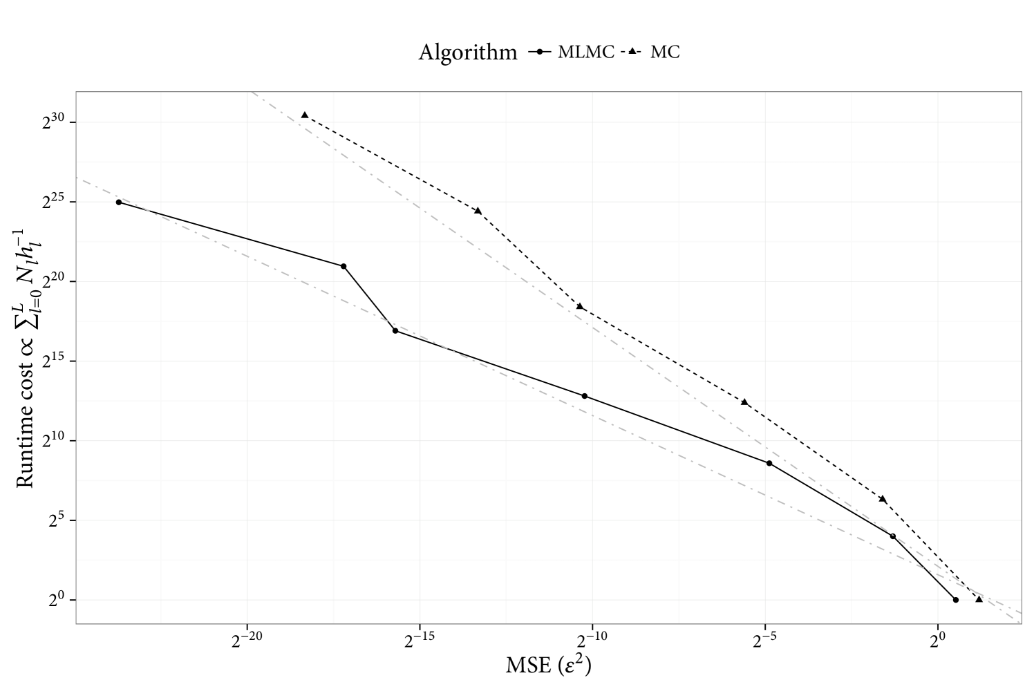
For problems which must first be approximated at finite resolution, as is the case in this article, and must subsequently be sampled from using MC-based methods, a multilevel (ML) framework may be used. This can potentially reduce the cost to obtain a given level of mean square error (MSE) [14, 11, 12], relative to performing i.i.d. sampling from the approximate posterior at a given (high) resolution. A telescopic sum of successively refined approximation increments are estimated instead of a single highly resolved approximation. The convergence of the refined approximation increments allows one to balance the cost between levels, and optimally obtain a cost $\mathcal{O}(\varepsilon^{-2})$ for MSE $\mathcal{O}(\varepsilon^{2})$ . This is shown in the context of the models in this article. Specifically, it is shown that the cost of MLMC, to provide a MSE of $\mathcal{O}(\varepsilon^{2})$ , is less than i.i.d. sampling from the most accurate prior approximation.

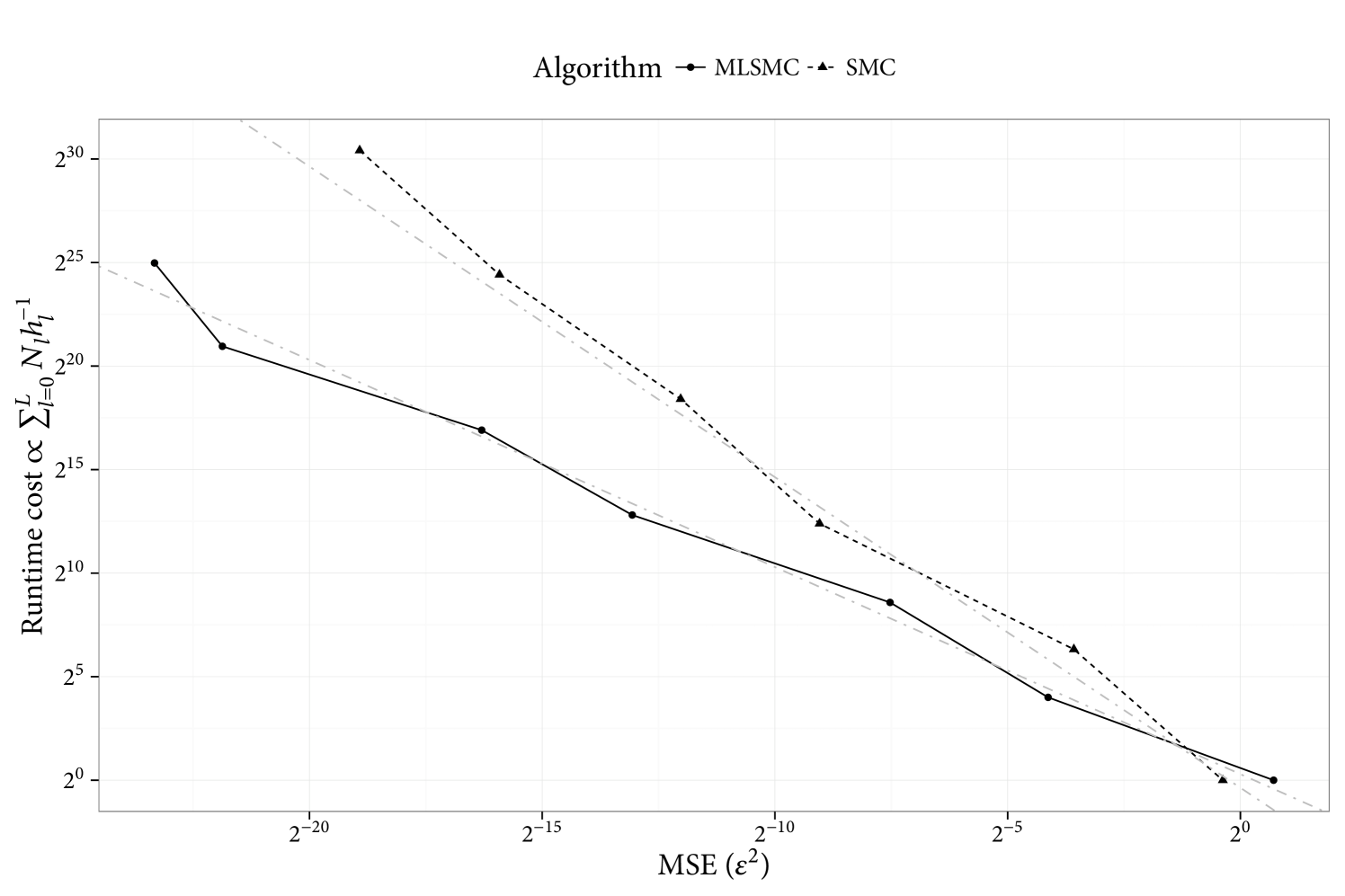
SMC within the ML framework has been primarily developed in [3, 9, 16]. These methodologies, some of which consider a similar context to this article, have been introduced where the ML approach is thought to be beneficial, but i.i.d. sampling is not possible. Indeed, one often has to resort to advanced MCMC or SMC methods to implement the ML identity; see for instance [15] for MCMC. SMC for nonlocal problems however, is a very sensible framework to implement the ML identity, as it will approximate a sequence of related probabilities of increasing complexity; in some cases, exact simulation from couples of the probabilities is not possible. As a result, SMC is the computational framework which we will primarily pursue in this article. It is shown that the cost of MLSMC, to provide a MSE of $\mathcal{O}(\varepsilon^{2})$ , is less than i.i.d. sampling from the most accurate posterior approximation. It is noted, however, that some developments both with regards to theoretical analysis and implentation of the algorithm, must be carefully considered in order to successfully use MLSMC for nonlocal models.

This article is structured as follows. In section 2 the nonlocal elliptic equations are given, along with the Bayesian inverse problem, and well-posedness of both are established. In particular, it is shown that the posterior has a well-defined Radon-Nikodym derivative w.r.t. prior measure. In section 3 we consider how one can approximate expectations w.r.t. the prior and the posterior, specifically using MLMC and MLSMC methods. Our complexity results are given also. Section 4 provides some numerical implementations of MLMC and MLSMC for the prior, and posterior, respectively.

2 Nonlocal elliptic equations

2.1 Setup

Consider the following equation

	$\displaystyle\mathcal{L}(u)(x)$	$\displaystyle=$	$\displaystyle b(x),\quad{\rm for~}x\in\Omega\subset\mathbb{R}^{d}$		(2.1)
	$\displaystyle u(x)$	$\displaystyle=$	$\displaystyle 0,\quad{\rm for~}x\in\Gamma,$		(2.2)

where $\mathcal{L}$ is given by (1.1), the domain $\Omega$ is simply connected, and its “boundary” $\Gamma$ is sufficiently regular and nonlocal, in the sense that it has non-zero volume in $\mathbb{R}^{d}$ ,

Under appropriate conditions on $B$ , $\mathcal{L}^{-1}:H^{-s}(\Omega\cup\Gamma)\rightarrow H^{s}_{c}(\Omega\cup\Gamma)$ , for $s\in[0,1)$ , with $s=1$ only for the limiting local version in which $B(x,x^{\prime})=(I-\partial^{2}/\partial x^{2})\delta(x^{\prime}-x)$ (or a similar uniformly elliptic form) [10]. Following [10] $H^{s}_{c}=\{u\in H^{s};u|_{\Gamma}=0,\int_{\mathbb{R}^{d}}u(x)dx=0\}$ denotes the volume constrained space of functions, and the fractional Sobolev space $H^{s}$ is defined as follows, for $s\in(0,1)$ ,

H^{s}:=\{u\in L^{2}(\Omega\cup\Gamma):\|u\|_{L^{2}(\Omega\cup\Gamma)}+|u|_{H^{s}(\Omega\cup\Gamma)}<\infty\},

(2.3)

where

|u|_{H^{s}(\Omega\cup\Gamma)}:=\int_{\Omega\cup\Gamma}\int_{\Omega\cup\Gamma}\frac{(u(x)-u(y))^{2}}{|x-y|^{d+2s}}dydx.

We define $H^{0}_{c}:=L^{2}_{c}$ for ease of notation.

For $b\in V^{*}(\Omega\cup\Gamma)$ , the dual with respect to $L^{2}$ of some space $V(\Omega\cup\Gamma)$ , the weak formulation of (2.2) can be defined as follows. Integrate the equation against an arbitrary test function $v\in V(\Omega\cup\Gamma)$ . Now, find $u\in V(\Omega\cup\Gamma)$ (satisfying the boundary conditions) such that

\displaystyle\mathcal{B}(u,v)

\displaystyle=F(v),\quad{\rm for~all~}v\in V(\Omega\cup\Gamma),

(2.4)

where

\begin{split}\mathcal{B}(u,v)&:=\int_{\mathbb{R}^{d}}\int_{\mathbb{R}^{d}}[u(x^{\prime})-u(x)]B(x,x^{\prime})dx^{\prime}v(x)dx,\\ F(v)&:=\int_{\mathbb{R}^{d}}b(x)v(x)dx.\end{split}

2.2 Numerical methods for forward solution

Let $h_{\ell}$ denote the maximum diameter of an element of $V_{\ell}\subset V_{\ell+1}\subset\cdots\subset V$ . The finite approximation of (2.4) is stated as follows. Identify some $u_{\ell}\in V_{\ell}$ such that

\displaystyle\mathcal{B}(u_{\ell},v_{\ell})

\displaystyle=F(v_{\ell}),\quad{\rm for~all~}v_{\ell}\in V_{\ell}.

(2.5)

Assuming the spaces $V_{\ell}$ are spanned by elements $\{\phi^{k}_{\ell}\}_{k=1}^{M_{\ell}}$ , then one can substitute the ansatz $u_{\ell}=\sum_{k=1}^{M_{\ell}}u_{\ell}^{k}\phi^{k}_{\ell}$ into the above equation, resulting in the finite linear system

\displaystyle\sum_{k=1}^{M_{\ell}}\mathcal{B}(\phi_{\ell}^{j},\phi^{k}_{\ell})u_{k}

\displaystyle=F(\phi_{\ell}^{j}),\quad{\rm for~}j=1,\dots,M_{\ell}.

(2.6)

In particular, the spaces $\{V_{\ell}\}$ will be comprised of discontinuous elements, so that the method described is a discontinuous Galerkin finite element method (FEM) [4]. Piecewise polynomial discontinuous element spaces are dense in $H^{s}_{c}$ for $s\in[0,1/2)$ , and are therefore conforming when $u\in H_{c}^{s}=V$ for $s\in[0,1/2)$ , so there is no need to impose penalty terms at the boundaries as one must do for smoother problems in which the discontinuous elements are non-conforming.

2.3 Forward UQ

The following assumption will be made for simplicity

Assumption 2.1.

$V=L^{2}(\Omega\cup\Gamma)$ , with norm $\|\cdot\|$ and inner product $\langle\cdot,\cdot\rangle$ . $B(x,x^{\prime})=B(|x^{\prime}-x|)\geq 0$ is continuous with $B(0)\geq c^{\prime}>0$ , and there exist $K_{1}>0$ such that for all $x\in\Omega$

\displaystyle\int_{\Omega\cup\Gamma}B(x,x^{\prime})dx^{\prime}

\displaystyle\leq K_{1}.

(2.7)

As shown in Section 6 of [13], this implies that for all $u,v,b\in V$

•

$F$ is continuous: $|F(v)|\leq\|b\|\|v\|$ ;
•

$\mathcal{B}$ is continuous: $|\mathcal{B}(u,v)|\leq 4K_{1}\|u\|\|v\|$ ;
•

$\mathcal{B}$ is coercive: $|\mathcal{B}(u,u)|\geq K_{2}\|u\|^{2}$ for some $K_{2}(\mathcal{B},\Omega)>0$ . This actually follows from the Poincaré-type inequality derived in Proposition 2.5 of [1].

Hence, Lax-Milgram lemma ([5], Thm. 1.1.3) can be invoked, guaranteeing existence of a unique solution $u\in L^{2}(\Omega)$ such that

\|u\|\leq K_{2}^{-1}\|b\|.

In other words, the map $b\mapsto u$ is continuous. The system (2.6) inherits solvability since the bilinear is a fortiori coercive on $V_{\ell}$ , so that

\|u_{\ell}\|\leq K_{2}^{-1}\|b\|.

Let $B_{\lambda}$ be a parametrization of $B$ , where $\lambda\sim\mu_{0}$ and $\lambda\in E$ , and either $E=\mathbb{R}^{p}$ or $E\subset\mathbb{R}^{p}$ compact. Then the following theorem holds.

Theorem 2.2 (Well-posedness of forward UQ).

If Assumption 2.1 holds almost surely for $\lambda\sim\mu$ and the map $u\mapsto Q$ is continuous from $L^{2}$ to $\mathbb{R}$ , then the map $\lambda\mapsto Q$ is almost surely continuous. Hence $Q(\lambda)\in L^{\infty}\supset L^{p}$ for all $p\geq 1$ , i.e. all moments exist. $L^{p}$ here denotes the space of random variables $X$ such that $\int_{E}|X|^{p}\mu(d\lambda)<\infty$ .

Proof.

Since Assumption 2.1 holds almost surely for $\lambda\sim\mu$ , then $\|u\|\leq u^{*}:=K_{2}^{-1}\|b\|$ uniformly. So, the quantity of interest $Q(\lambda)=\|u(\lambda)\|\in L^{\infty}\supset L^{p}$ for all $p\geq 1$ . Therefore, for any $Q:L^{2}(\Omega)\rightarrow\mathbb{R}$ such that $Q(\lambda):=Q(u(\lambda))\leq K\|u\|$ , the result follows, since then $Q(\lambda)\leq Q^{*}:=Ku^{*}$ for all $\lambda$ . ∎

Corollary 2.3 (Well-posedness of finite approximation).

If Assumption 2.1 holds almost surely for $\lambda\sim\mu$ and the map $u_{\ell}\mapsto Q_{\ell}$ is continuous from $L^{2}$ to $\mathbb{R}$ , then the map through the discrete system $\lambda\mapsto Q_{\ell}$ is almost surely continuous and $Q_{\ell}\in L^{\infty}$ .

2.4 Inverse UQ

For the inverse problem, let us assume that some data is given in the form

y=\mathcal{G}(\lambda)+\xi,\quad\lambda\perp\xi\sim N(0,\Sigma),

(2.8)

where

\mathcal{G}(\lambda):=[\langle g_{1},u(\lambda)\rangle,\dots,\langle g_{M},u(\lambda)\rangle]^{\top},\quad g_{i}\in V.

(2.9)

Then the following theorem holds.

Theorem 2.4 (Well-posedness of inverse UQ).

The posterior distribution of $\lambda|y$ is well-defined and takes the form

\frac{d\eta^{y}}{d\mu}(\lambda)=\frac{1}{Z}\exp\{-\frac{1}{2}|\Sigma^{-1/2}(\mathcal{G}(\lambda)-y)|^{2}\},

(2.10)

with $Z=\int_{E}\exp\{-\frac{1}{2}|\Sigma^{-1/2}(\mathcal{G}(\lambda)-y)|^{2}\}\mu(d\lambda)$ .

Proof.

The form of the posterior is obtained by a change of variables to $\{\lambda,\xi=y-\mathcal{G}(\lambda)$ }, which are independent by assumption. Note the change of variables has Jacobian 1. So, changing variables back, this also gives the joint density. The posterior is obtained by normalizing for the observed value of $y$ . The form of the observation operator guarantees $Z>\exp\{-|\Sigma^{-1}|(|\mathcal{G}^{*}|^{2}+|y|^{2})\}$ , where $\mathcal{G}^{*}=(\mathcal{G}_{1}^{*},\mathcal{G}_{2}^{*},\dots,\mathcal{G}_{M}^{*})$ and $\mathcal{G}_{i}^{*}$ is defined as in the proof of Theorem 2.2, and $|\Sigma^{-1}|$ is the matrix norm. ∎

Now define $\mathcal{G}_{\ell}(\lambda):=[\langle g_{1},u_{\ell}(\lambda)\rangle,\dots,\langle g_{M},u_{\ell}(\lambda)\rangle],\quad g_{i}\in L^{2}(\Omega).$

Corollary 2.5 (Well-posedness of inverse UQ for finite problem).

The finite approximation of the posterior distribution of $\lambda|y$ is well-defined and takes the form

\frac{d\eta^{y}_{\ell}}{d\mu}(\lambda)=\frac{1}{Z}\exp\{-\frac{1}{2}|\Sigma^{-1/2}(\mathcal{G}_{\ell}(\lambda)-y)|^{2}\},

(2.11)

with $Z_{\ell}=\int_{E}\exp\{-\frac{1}{2}|\Sigma^{-1/2}(\mathcal{G}_{\ell}(\lambda)-y)|^{2}\}\mu(d\lambda)$ .

Remark 2.6.

The forcing may also be taken as uncertain, although the uniformity will require it to be defined on a compact space. The probability space $E$ will be taken as compact for simplicity, as it is then easy to verify Assumption 2.1.

3 Approximation of expectations

The objective here is to approximate expectations of some functional $\varphi:E\rightarrow\mathbb{R}$ with respect to a probability measure $\eta$ ( $\mu$ or $\eta^{y}$ ), denoted $\mathbb{E}_{\eta}(\varphi).$ The solution $u$ of (2.2) above must be approximated by some $u_{\ell}$ , with a degree of accuracy which depends on $\ell$ . Indeed there exists a hierarchy of levels $\ell=0,\dots,L$ (where $L$ may be arbitrarily large) of increasing accuracy and increasing cost. For the inverse problem this manifests in a hierarchy of target probability measures $\{\eta_{\ell}\}_{\ell=0}^{L}$ via the approximation of (2.10). For the forward problem $\eta_{\ell}=\eta$ for all $\ell$ , but it will be assumed that the function $\varphi$ requires evaluation of the solution of (2.2), as in Theorem 2.2, and the corresponding approximations will be denoted by $\{\varphi_{\ell}\}_{\ell=0}^{L}$ . One may then compute the estimator $\hat{Y}_{L}^{N}=\frac{1}{N}\sum_{n=1}^{N}\varphi_{L}(\lambda_{L}^{n}),\lambda_{L}^{n}\sim\eta_{L}$ , where for the forward problem it may be that $\eta_{L}\equiv\eta$ for all $L$ . The mean square error (MSE) is given by

\mathbb{E}\left|\mathbb{E}_{\eta}[\varphi(\lambda)]-\hat{Y}_{L}^{N}\right|^{2}=\underbrace{\mathbb{E}\left\{\mathbb{E}_{\eta_{L}}[\varphi_{L}(\lambda)]-\hat{Y}_{L}^{N}\right\}^{2}}_{\rm variance}+\underbrace{\{\mathbb{E}_{\eta_{L}}[\varphi_{L}(\lambda)]-\mathbb{E}_{\eta}[\varphi(\lambda)]\}^{2}}_{\rm bias}\ .

(3.1)

Now assume there is some discretization level, say of diameter $h_{L}$ , which gives rise to an error estimate on the output of size $\mathcal{O}(h_{L}^{\alpha})$ , for example arising from the deterministic numerical approximation of a spatio-temporal problem. This also translates to a number of degrees of freedom proportional to $h_{L}^{-d}$ , where $d$ is the spatio-temporal dimension. Now the complexity of typical forward solves will range from a dot product $\mathcal{O}(h_{L}^{-d})$ (linear) to a full Gaussian elimination $\mathcal{O}(h_{L}^{-3d})$ (cubic). In this problem one aims to find $h_{L}^{\alpha}=\mathcal{O}(\varepsilon)$ , so one would find the cost controlled by $\mathcal{O}(\varepsilon^{-\zeta/\alpha})$ , for $\zeta\in(d,3d)$ . If one can obtain independent, identically distributed samples $u^{n}_{L}$ , then the necessary number of samples to obtain a variance of size $\mathcal{O}(\varepsilon^{2})$ is given by $N=\mathcal{O}(\varepsilon^{-2})$ . The total cost to obtain a mean-square error tolerance of $\mathcal{O}(\varepsilon^{2})$ is therefore $\mathcal{O}(\varepsilon^{-2-\zeta/\alpha})$ .

3.1 Multilevel Monte Carlo

For the forward UQ problem, in which one can sample directly from $\eta_{\ell}$ , one very popular methodology for improving the efficiency of solution to such problems is the multilevel Monte Carlo (MLMC) method [14, 11]. Indeed there has been an explosion of recent activity [12] since its introduction in [11]. In this methodology the simple estimator $\hat{Y}_{L}^{N}$ above for a given desired $L$ is replaced by a telescopic sum of unbiased increment estimators $Y^{N_{\ell}}_{\ell}=\sum_{i=1}^{N_{\ell}}\{\varphi_{\ell}(\lambda_{\ell}^{(i)})-\varphi_{\ell-1}(\lambda_{\ell-1}^{(i)})\}N_{\ell}^{-1}$ where $\{\lambda_{\ell-1}^{(i)},\lambda_{\ell}^{(i)}\}$ are i.i.d. samples, with marginal laws $\eta_{\ell-1}$ , $\eta_{\ell}$ , respectively, carefully constructed on a joint probability space. This is repeated independently for $0\leq\ell\leq L$ . The overall multilevel estimator will be

\hat{Y}_{L,{\rm Multi}}=\sum_{\ell=0}^{L}Y^{N_{\ell}}_{\ell}\,,

(3.2)

under the convention that $g(\lambda_{-1}^{(i)})=0$ . A simple error analysis shows that the mean squared error (MSE) in this case is given by

	$\displaystyle\mathbb{E}\{\hat{Y}_{L,{\rm Multi}}-\mathbb{E}_{\eta}[\varphi(\lambda)]\}^{2}$	$\displaystyle=\underbrace{\sum_{\ell=0}^{L}\mathbb{E}\left\{Y^{N_{\ell}}_{\ell}-[\mathbb{E}_{\eta_{\ell}}{\varphi_{\ell}}(\lambda)-\mathbb{E}_{\eta_{\ell-1}}{\varphi_{\ell-1}}(\lambda)]\right\}^{2}}_{\rm variance}$			(3.3)
		$\displaystyle+\underbrace{\{\mathbb{E}_{\eta_{L}}[{\varphi_{L}}(\lambda)]-\mathbb{E}_{\eta}[\varphi(\lambda)]\}^{2}}_{\rm bias}\ .$			(3.3)

Notice that the bias is given by the finest level, whilst the variance is decomposed into a sum of variances of the increments. The variance of the $\ell^{th}$ increment estimator has the form $\mathcal{V}_{\ell}N_{\ell}^{-1}$ , where the terms $\mathcal{V}_{\ell}=\mathbb{E}|\varphi_{\ell}(\lambda_{\ell})-\varphi_{\ell-1}(\lambda_{\ell-1})|^{2}$ decay, following from refinement of the approximation of $\eta$ and/or $\varphi$ . One can therefore balance the variance at a given level $\mathcal{V}_{\ell}$ with the number of samples $N_{\ell}$ . As the level increases, the corresponding cost increases, but the variance decreases, allowing fewer samples to achieve a given variance. This can be optimized, and results in a total cost of $\mathcal{O}(\varepsilon^{-\max\{2,\zeta/\alpha\}})$ , in the optimal case.

To be explicit, denote by $Q_{\ell}:=Q(u_{\ell}(\lambda_{\ell}),\lambda_{\ell})$ the level $\ell$ approximation of the quantity of interest $Q$ . Introduce the following assumptions

(A1)

There exist $\alpha,\beta,\zeta>0$ , and a $C>0$ such that

\begin{cases}|\mathbb{E}(Q_{L}-Q_{\infty})|&\leq Ch_{L}^{\alpha};\\ \mathbb{E}|Q_{\ell}-Q_{\ell-1}|^{2}&\leq Ch_{\ell}^{\beta};\\ {\rm C}(Q_{\ell})&\leq Ch_{\ell}^{-\zeta},\end{cases}

(3.4)

where ${\rm C}(Q_{\ell})$ denotes the cost to evaluate $Q_{\ell}$ .

We have the following classical MLMC Theorem [12]

Theorem 3.1.

Assume (A(A1)) and $\rm{max}\{\beta,\zeta\}\leq 2\alpha$ . Then for any $\varepsilon>0$ , there exist $L,\{N_{\ell}\}_{\ell=0}^{L}$ and $C>0$ such that

\mathbb{E}\Big{[}\Big{(}\hat{Y}_{L,{\rm Multi}}-\mathbb{E}_{\eta}[Q]\Big{)}^{2}\Big{]}\leq C\varepsilon^{2},

(3.5)

for the following cost

{\rm COST}\leq C\begin{cases}\varepsilon^{-2},&\text{if}\quad\beta>\zeta,\\ \varepsilon^{-2}|\log(\varepsilon)|^{2},&\text{if}\quad\beta=\zeta,\\ \varepsilon^{-\left(2+\frac{\zeta-\beta}{\alpha}\right)},&\text{if}\quad\beta<\zeta.\end{cases}

(3.6)

3.2 Multilevel sequential Monte Carlo sampler

Now the inverse problem will be considered. There is a sequence of probability measures $\{\eta_{\ell}\}_{\ell\geq 0}$ on a common measurable space $(E,\mathcal{E})$ , and for each $l$ there is a measure $\gamma_{\ell}:\mathcal{E}\rightarrow\mathbb{R}^{+}$ , such that

\eta_{\ell}(d\lambda)=\frac{\gamma_{\ell}(d\lambda)}{Z_{\ell}}

(3.7)

where the normalizing constant $Z_{\ell}=\int_{E}\gamma_{\ell}(d\lambda)$ is unknown. The objective is to compute:

\mathbb{E}_{\eta_{\infty}}[\varphi(\lambda)]:=\int_{E}\varphi(\lambda)\eta_{\infty}(d\lambda)

for potentially many measurable $\eta_{\infty}-$ integrable functions $\varphi:E\rightarrow\mathbb{R}$ .

3.2.1 Notations

Let $(E,\mathcal{E})$ be a measurable space. The notation $\mathcal{B}_{b}(E)$ denotes the class of bounded and measurable real-valued functions, and the supremum norm is written as $\|f\|_{\infty}=\sup_{\lambda\in E}|f(\lambda)|$ . Consider non-negative operators $K:E\times\mathcal{E}\rightarrow\mathbb{R}_{+}$ such that for each $\lambda\in E$ the mapping $A\mapsto K(\lambda,A)$ is a finite non-negative measure on $\mathcal{E}$ and for each $A\in\mathcal{E}$ the function $\lambda\mapsto K(\lambda,A)$ is measurable; the kernel $K$ is Markovian if $K(\lambda,dv)$ is a probability measure for every $\lambda\in E$ . For a finite measure $\mu$ on $(E,\mathcal{E})$ , and a real-valued, measurable $f:E\rightarrow\mathbb{R}$ , we define the operations:

\mu K:A\mapsto\int K(\lambda,A)\,\mu(d\lambda)\ ;\quad Kf:\lambda\mapsto\int f(v)\,K(\lambda,dv).

We also write $\mu(f)=\int f(\lambda)\mu(d\lambda)$ . In addition $\|\cdot\|_{r}$ , $r\geq 1$ , denotes the $L_{r}-$ norm, where the expectation is w.r.t. the law of the appropriate simulated algorithm.

3.2.2 Algorithm

As described in Section 1, the context of interest is when a sequence of densities $\{\eta_{\ell}\}_{\ell\geq 0}$ , as in (3.7), are associated to an ‘accuracy’ parameter $h_{l}$ , with $h_{\ell}\rightarrow 0$ as $\ell\rightarrow\infty$ , such that $\infty>h_{0}>h_{1}\cdots>h_{\infty}=0$ . In practice one cannot treat $h_{\infty}=0$ and so must consider these distributions with $h_{\ell}>0$ . The laws with large $h_{\ell}$ are easy to sample from with low computational cost, but are very different from $\eta_{\infty}$ , whereas, those distributions with small $h_{\ell}$ are hard to sample with relatively high computational cost, but are closer to $\eta_{\infty}$ . Thus, we choose a maximum level $L\geq 1$ and we will estimate

\mathbb{E}_{\eta_{L}}[\varphi(\lambda)]:=\int_{E}\varphi(\lambda)\eta_{L}(\lambda)d\lambda\ .

By the standard telescoping identity used in MLMC, one has

	$\displaystyle\mathbb{E}_{\eta_{L}}[\varphi(\lambda)]$	$\displaystyle=\mathbb{E}_{\eta_{0}}[\varphi(\lambda)]+\sum_{\ell=1}^{L}\Big{\{}\mathbb{E}_{\eta_{\ell}}[\varphi(\lambda)]-\mathbb{E}_{\eta_{\ell-1}}[\varphi(\lambda)]\Big{\}}$
		$\displaystyle=\mathbb{E}_{\eta_{0}}[\varphi(\lambda)]+\sum_{\ell=1}^{L}\mathbb{E}_{\eta_{\ell-1}}\Big{[}\Big{(}\frac{\gamma_{\ell}(\lambda)Z_{\ell-1}}{\gamma_{\ell-1}(\lambda)Z_{\ell}}-1\Big{)}\varphi(\lambda)\Big{]}\ .$		(3.8)

Suppose now that one applies an SMC sampler [8] to obtain a collection of samples (particles) that sequentially approximate $\eta_{0},\eta_{1},\ldots,\eta_{L}$ . We consider the case when one initializes the population of particles by sampling i.i.d. from $\eta_{0}$ , then at every step resamples and applies a MCMC kernel to mutate the particles. We denote by $(\lambda_{0}^{1:N_{0}},\dots,\lambda_{L-1}^{1:N_{L-1}})$ , with $+\infty>N_{0}\geq N_{1}\geq\cdots N_{L-1}\geq 1$ , the samples after mutation; one resamples $\lambda_{l}^{1:N_{l}}$ according to the weights $G_{\ell}(\lambda_{\ell}^{i})=(\gamma_{\ell+1}/\gamma_{\ell})(\lambda_{\ell}^{i})$ , for indices $l\in\{0,\dots,L-1\}$ . We will denote by $\{M_{\ell}\}_{1\leq\ell\leq L-1}$ the sequence of MCMC kernels used at stages $1,\dots,L-1$ , such that $\eta_{\ell}M_{\ell}=\eta_{\ell}$ . For $\varphi:E\rightarrow\mathbb{R}$ , $\ell\in\{1,\dots,L\}$ , we have the following estimator of $\mathbb{E}_{\eta_{\ell-1}}[\varphi(\lambda)]$ :

\eta_{\ell-1}^{N_{\ell-1}}(\varphi)=\frac{1}{N_{\ell-1}}\sum_{i=1}^{N_{\ell-1}}\varphi(\lambda_{\ell-1}^{i})\ .

We define

\eta_{\ell-1}^{N_{\ell-1}}(G_{\ell-1}M_{\ell}(d\lambda_{\ell}))=\frac{1}{N_{\ell-1}}\sum_{i=1}^{N_{\ell-1}}G_{\ell-1}(\lambda_{\ell-1}^{i})M_{\ell}(\lambda_{\ell-1}^{i},d\lambda_{\ell})\ .

The joint probability distribution for the SMC algorithm is

\prod_{i=1}^{N_{0}}\eta_{0}(d\lambda_{0}^{i})\prod_{\ell=1}^{L-1}\prod_{i=1}^{N_{\ell}}\frac{\eta_{\ell-1}^{N_{\ell-1}}(G_{\ell-1}M_{\ell}(d\lambda_{\ell}^{i}))}{\eta_{\ell-1}^{N_{\ell-1}}(G_{\ell-1})}\ .

If one considers one more step in the above procedure, that would deliver samples $\{\lambda_{L}^{i}\}_{i=1}^{N_{L}}$ , a standard SMC sampler estimate of the quantity of interest in (3.8) is $\eta_{L}^{N}(g)$ ; the earlier samples are discarded. Within a multilevel context, a consistent SMC estimate of (3.8) is

\widehat{Y}=\eta_{0}^{N_{0}}(\varphi)+\sum_{\ell=1}^{L}\Big{\{}\frac{\eta_{\ell-1}^{N_{\ell-1}}(\varphi G_{\ell-1})}{\eta_{\ell-1}^{N_{\ell-1}}(G_{\ell-1})}-\eta_{\ell-1}^{N_{\ell-1}}(\varphi)\Big{\}}\ ,

(3.9)

and this will be proven to be superior than the standard one, under assumptions.

The relevant MSE error decomposition here is:

\mathbb{E}\big{[}\{\widehat{Y}-\mathbb{E}_{\eta_{\infty}}[\varphi(\lambda)]\}^{2}\big{]}\leq 2\,\mathbb{E}\big{[}\{\widehat{Y}-\mathbb{E}_{\eta_{L}}[\varphi(\lambda)]\}^{2}\big{]}+2\,\{\mathbb{E}_{\eta_{L}}[\varphi(\lambda)]-\mathbb{E}_{\eta_{\infty}}[\varphi(\lambda)]\}^{2}\ .

(3.10)

3.2.3 Multilevel SMC

We will now restate an analytical result from [3] that controls the error term $\mathbb{E}[\{\widehat{Y}-\mathbb{E}_{\eta_{L}}[\varphi(\lambda)]\}^{2}]$ in expression (3.10). For any $\ell\in\{0,\dots,L\}$ and $\varphi\in\mathcal{B}_{b}(E)$ we write: $\eta_{\ell}(\varphi):=\int_{E}\varphi(\lambda)\eta_{\ell}(\lambda)d\lambda.$ The following standard assumptions will be made ; see [3, 7].

(A2)

There exist $0<\underline{C}<\overline{C}<+\infty$ such that

	$\displaystyle\sup_{\ell\geq 1}\sup_{\lambda\in E}G_{\ell}(\lambda)$	$\displaystyle\leq$	$\displaystyle\overline{C}\ ;$
	$\displaystyle\inf_{\ell\geq 1}\inf_{\lambda\in E}G_{\ell}(\lambda)$	$\displaystyle\geq$	$\displaystyle\underline{C}\ .$

(A3)

There exists a $\rho\in(0,1)$ such that for any $\ell\geq 1$ , $(\lambda,v)\in E^{2}$ , $A\in\mathcal{E}$ :

$\int_{A}M_{\ell}(\lambda,d\lambda^{\prime})\geq\rho\int_{A}M_{\ell}(v,d\lambda^{\prime})\ .$

Under these assumptions the following Theorem is proven in [3]

Theorem 3.2.

Assume (A(A2)-(A3)). There exist $C<+\infty$ such that for any $\varphi\in\mathcal{B}_{b}(E)$ , with $\|\varphi\|_{\infty}=1$ ,

\displaystyle\mathbb{E}\big{[}\{\widehat{Y}-\mathbb{E}_{\eta_{L}}[\varphi(\lambda)]\}^{2}\big{]}\leq C\,\bigg{(}\frac{1}{N_{0}}+

\displaystyle\sum_{\ell=1}^{L}\bigg{(}\tfrac{\mathcal{V}_{l}}{N_{l-1}}+\tfrac{\mathcal{V}_{\ell}^{1/2}}{N_{\ell-1}^{1/2}}\sum_{q=\ell+1}^{L}\tfrac{\mathcal{V}_{q}^{1/2}}{N_{q-1}}\bigg{)}\bigg{)}\ ,

where $\mathcal{V}_{\ell}:=\|\tfrac{Z_{\ell-1}}{Z_{\ell}}G_{\ell-1}-1\|_{\infty}^{2}$ .

The following additional assumption will now be made

(A4)

There exist $\alpha,\beta,\zeta>0$ , and a $C>0$ such that

\begin{cases}\mathcal{V}_{\ell}&\leq Ch_{\ell}^{\beta};\\ |(\eta_{L}-\eta_{\infty})(1)|&\leq Ch_{L}^{\alpha};\\ {\rm C}(G_{\ell})&\leq Ch_{\ell}^{-\zeta},\end{cases}

(3.11)

where ${\rm C}(G_{\ell})$ denotes the cost to evaluate $G_{\ell}$ .

The following Theorem may now be proven

Theorem 3.3.

Assume (A(A2)-(A4)) and $\rm{max}\{\beta,\zeta\}\leq 2\alpha$ . Then for any $\varepsilon>0$ , there exist $L,\{N_{\ell}\}_{\ell=0}^{L}$ and $C>0$ such that

\mathbb{E}\Big{[}\Big{(}\widehat{Y}-\mathbb{E}_{\eta}[\varphi(\lambda)]\Big{)}^{2}\Big{]}\leq C\varepsilon^{2},

(3.12)

for the following cost

{\rm COST}\leq C\begin{cases}\varepsilon^{-2},&\text{if}\quad\beta>\zeta,\\ \varepsilon^{-2}|\log(\varepsilon)|^{2},&\text{if}\quad\beta=\zeta,\\ \varepsilon^{-\left(2+\frac{\zeta-\beta}{\alpha}\right)},&\text{if}\quad\beta<\zeta.\end{cases}

(3.13)

Proof.

The MSE can be bounded using (3.10). Following from (A(A4))(ii), the second term requires that $h_{L}^{\alpha}\eqsim\varepsilon$ , and assuming $h_{L}=M^{-L}$ for some $M\geq 2$ , this translates to $L\eqsim\log\varepsilon$ . As in [3], the additional error term is dealt with by first ignoring it and optimizing ${\rm COST}({\bf N})$ , for a given $\mathcal{V}({\bf N})=\varepsilon^{2}$ , where ${\bf N}:=(N_{1},\dots,N_{L})$ . This requires that $N_{\ell}\propto\sqrt{\mathcal{V}_{l}/C_{l}}\eqsim h_{\ell}^{(\beta+\zeta)/2}$ . The constraint then requires that $N_{\ell}=\varepsilon^{-2}K_{L}h_{\ell}^{(\beta+\zeta)/2}$ , where $K_{L}=\sum_{l=1}^{L-1}h_{l}^{(\beta-\zeta)/2}$ , so one has

{\rm COST}({\bf N})=\sum_{\ell=0}^{L}N_{\ell}C_{\ell}=\varepsilon^{-2}K_{L}^{2}.

It was shown in [3] that the result follows, provided $\zeta<2\alpha$ . In fact, re-examining the additional term as in Section 3.3 of [3], one has

\begin{split}\sum_{\ell=1}^{L}\tfrac{\mathcal{V}_{\ell}^{1/2}}{N_{\ell-1}^{1/2}}\sum_{q=\ell+1}^{L}\tfrac{\mathcal{V}_{q}^{1/2}}{N_{q-1}}&=\mathcal{O}(\varepsilon^{2}\varepsilon^{1-\zeta/2\alpha}\sum_{\ell=1}^{L-1}h_{\ell}^{(\beta-\zeta)/4}K_{L}^{-3/2})\\ &=\mathcal{O}(\varepsilon^{2}\varepsilon^{1-\zeta/2\alpha}L^{1/2}K_{L}^{-1}),\end{split}

where the second line follows from the inequality $(\sum_{\ell=0}^{L}a_{\ell})^{2}\leq L\sum_{\ell=0}^{L}a_{\ell}^{2}$ and the definition of $K_{L}$ . Now substituting $K_{L}=\mathcal{O}(1),\mathcal{O}(L),\mathcal{O}(\varepsilon^{-(\zeta-\beta)/2\alpha})$ for the 3 cases and recalling the assumption $\rm{max}\{\beta,\zeta\}\leq 2\alpha$ gives $\mathcal{V}({\bf N})=\varepsilon^{2}$ for the costs in (3.13).

∎

3.2.4 Verification of assumptions

Assume a uniform prior $\mu$ . Following from (2.8), the unnormalized measures will be given by

\gamma_{\ell}=\exp\{-\Phi(\mathcal{G}_{\ell}(\lambda))\},

(3.14)

where $\Phi(\mathcal{G}_{l}(\lambda))=\frac{1}{2}|\Sigma^{-1/2}(\mathcal{G}_{l}(\lambda)-y)|^{2}$ , and

\mathcal{G}_{\ell}(\lambda):=[\langle g_{1},u_{\ell}(\lambda)\rangle,\dots,\langle g_{M},u_{\ell}(\lambda)\rangle]^{\top},\quad g_{i}\in L^{2}(\Omega),

and $u_{l}$ is the solution of the numerical approximation of (2.2). Notice that these are uniformly bounded, over both $\lambda\in E$ and over $\ell$ , following from Corollary 2.5 for finite $\ell$ , and Theorem 2.4 in the limit.

It is shown in [3] Section 4 that

|\Phi(\mathcal{G}_{\ell}(\lambda))-\Phi(\mathcal{G}_{\ell-1}(\lambda))|\leq C(|\mathcal{G}_{\ell}|,|\mathcal{G}_{\ell-1}|)|\mathcal{G}_{\ell}(\lambda)-\mathcal{G}_{\ell-1}(\lambda)|.

(3.15)

One proceeds similarly to that paper, and finds that

|\mathcal{G}_{\ell}(\lambda)-\mathcal{G}_{\ell-1}(\lambda)|\leq C\|u_{\ell}(\lambda)-u_{\ell-1}(\lambda)\|_{V}.

(3.16)

Note that $G_{\ell}=\gamma_{\ell+1}/\gamma_{\ell}$ , so inserting the bound (3.15) into (3.14), and observing the boundedness of the $\{\mathcal{G}_{\ell}\}$ noted above, one can see that Assumption (A(A2)) holds. Now inserting (3.15) and (3.16) into (3.14), one can see that in order to establish Assumption (A(A4)), it suffices to establish rates of convergence for $\|u_{\ell}(\lambda)-u_{\ell-1}(\lambda)\|_{V}$ . In particular, Assumption (A(A2)) and the C2 inequality (Minkowski plus Young’s) provide that

\begin{split}\mathcal{V}_{\ell}&=\|\tfrac{Z_{\ell-1}}{Z_{\ell}}G_{\ell-1}-1\|_{\infty}^{2}=\left\|\frac{G_{\ell-1}}{\eta_{\ell-1}(G_{\ell-1})}-1\right\|_{\infty}^{2}\\ &\leq C(\|{G_{\ell-1}}-1\|_{\infty}^{2}+\|\eta_{\ell-1}(G_{\ell-1})-1\|_{\infty}^{2})\leq 2C\|{G_{\ell-1}}-1\|_{\infty}^{2}\\ &\leq C^{\prime}\|u_{\ell}(\lambda)-u_{\ell-1}(\lambda)\|_{V}^{2}.\end{split}

Therefore, the rate of convergence of $\|u_{\ell}(\lambda)-u_{\ell-1}(\lambda)\|_{V}$ is the required quantity for both the forward (for Lipschitz $Q$ ) and the inverse multilevel estimation problems. By the triangle inequality it suffices to consider the approximation of the truth $\|u_{\ell}(\lambda)-u(\lambda)\|_{V}$ , and by Céa’s lemma ([5], Thm. 2.4.1), Assumption 2.1 guarantees the existence of a $C>0$ such that

\|u_{\ell}(\lambda)-u(\lambda)\|_{V}\leq C\inf_{v_{\ell}\in V_{\ell}}\|v_{\ell}(\lambda)-u(\lambda)\|_{V}

(3.17)

Theorem 6.2 of [10] provides rates of convergence of the best approximation above, in the case that $V=H^{s}$ and the FEM triangulation is shape regular and quasi-uniform. In particular, their Case 1 corresponds to the case of a singular kernel, i.e. not even integrable, and $\mathcal{L}:H^{s}_{c}\rightarrow H^{-s}$ , for $s\in(0,1)$ , so the solution operator is smoothing. Their Case 2 corresponds to a slightly more regular kernel than ours, where in fact $B(x,\cdot)\in L^{2}$ , rather than $L^{1}$ as given by Assumption 2.1 and consequently $\mathcal{L}:L^{2}_{c}\rightarrow L^{2}$ . It is shown that in Case 2, if the solution $u\in H^{m+t}$ , for polynomial elements of order $m$ and some $t\in[0,1]$ , then convergence with respect to the $L^{2}$ norm is in fact $\mathcal{O}(h^{m+t})$ . So, for linear elements, second order convergence can be obtained, leading to $\beta=4$ in (3.11).

Recall that 2.1 ensures well-posedness of the solution from $L^{2}\ni b\mapsto u\in L^{2}$ , and so discontinuities are allowed. This is actually a strength of nonlocal models and one impetus for their use. It is reasonable to expect that if the the nodes of the discontinuous elements match up with the discontinuities, i.e. there is a node at each point of discontinuity for $d=1$ or there are nodes all along a curve/surface of discontinuity for $d>1$ , and if the solution is sufficiently smooth in the subdomains, then the rates of convergence should match those of the smooth subproblems. For example, if there is a point discontinuity such that the domain can be separated at that point into $\Omega_{1}\cup\Omega_{2}=\Omega$ and one has $u|_{\Omega_{1}}\in H^{m+t}(\Omega_{1})$ and $u|_{\Omega_{2}}\in H^{m+t}(\Omega_{2})$ , where $u|_{\Omega_{i}}$ is the restriction of $u$ to the set $\Omega_{i}$ , then one expects the convergence rate of $m+t$ to be preserved. This is postulated and verified numerically in [4]. It is also illustrated numerically in that work that even with discontinuous elements, if there is no node at the discontinuity then the convergence rate reverts to $1/2$ , so $\beta=1$ in (3.11).

4 Numerical examples

The particular nonlocal model which will be of interest here is that in which the kernel is given by

B_{\lambda}(x,x^{\prime})=f(x,x^{\prime},\theta)\frac{1}{\delta^{2}|x-x^{\prime}|^{\alpha}}{\mathbf{1}}_{\{|x-x^{\prime}|<\delta\}},

(4.1)

where $\lambda:=(\theta,\alpha,\delta)$ , and ${\mathbf{1}}_{A}$ is the characteristic function which takes the value 1 if $(x,x^{\prime})\in A$ and zero otherwise, and $f(x,x^{\prime})=f(x^{\prime},x)$ . Notice that $\alpha\in(0,d)$ is scalar, but $(\theta,\delta)$ may be defined on either a finite-dimensional subspace of function-space, or in principle in the full infinite dimensional space. This may be of interest to incorporate spatial dependence of material properties.

Following [6] we consider the following model. Let $\Omega=[0,1]$ and $\Gamma=[-\delta,0)\cup(1,1+\delta]$ . For $(x,x^{\prime})\in\Omega^{2}$ , let $z=(x+x^{\prime})/2$ . The kernel is defined by,

	$\displaystyle f(x,x^{\prime},\theta)$	$\displaystyle=\begin{cases}0.2+(z-0.625)^{2}&\text{if }z\in[0,0.625)\\ z+\theta&\text{if }z\in[0.625,0.75)\\ 14.4+(z-0.75)+2&\text{if }z\in[0.75,1)\end{cases}$
	$\displaystyle b(x)$	$\displaystyle=5$

The following prior is used for the parameters,

	$\displaystyle\theta$	$\displaystyle\sim\mathrm{Uniform}(1,2)$
	$\displaystyle\alpha$	$\displaystyle\sim\mathrm{Beta}(2,2)$
	$\displaystyle\delta$	$\displaystyle\sim\mathrm{Gamma}(1,1)\text{ truncated on }(0.125,1)$

This is an extension of an example used in [6], which is identical to this model with $\theta=1.25$ and $\alpha=1$ (various values of $\delta$ are used there). To solve the equation with FEM, a uniform partition on $\Omega$ is used with $h_{\ell}=2^{-(k+\ell)}$ , $k=3$ . Thus for each level $\ell$ , $h<\delta$ . The same discontinuous Galerkin FEM as in [6] is applied to solve the system.

Similar methods to those in [3] are used to estimate the convergence rates for both the forward and inverse problems. The estimated rates are $\hat{\alpha}=2.005$ and $\hat{\beta}=4.271$ . The rates $\alpha=2$ and $\beta=4$ are used for the simulations.

For the inverse problem, data is generated with $\theta=2$ , $\alpha=0.5$ and $\delta=0.2$ . The observations are $y|u\sim N(m(u),\sigma^{2})$ , where $\sigma^{2}=0.01$ and $m(u)=[u(a),u(b)]^{\top}$ . The quantity of interest for both the forward and inverse problem is $u(0.5)$ .

The forward problem is solved in the standard multilevel fashion by generating coupled particles from the prior at each level. The main result, the cost vs. MSE of the estimates is shown in Figure 1. The Bayesian inverse problem is also solved for this model, and the main result is shown in Figure 2.

Refer to caption — Figure 1: Cost vs. MSE for MLMC

5 Summary

This is the first systematic treatment of UQ for nonlocal models, to the knowledge of the authors. Natural extensions include obtaining rigorous convergence results for piecewise smooth solutions, exploring higher-dimensional examples, spatial parameters, time-dependent models, and parameters defined on non-compact spaces.

Acknowledgements. KJHL was supported by the DARPA FORMULATE project. AJ & YZ were supported by Ministry of Education AcRF tier 2 grant, R-155-000-161-112. We express our gratitude to Marta D’Elia, Pablo Seleson, and Max Gunzburger for useful discussions.

References

[1] Andreu, F., Mazon, J. M., Jose, M. Rossi, J. & Toledo, J. (2009). A nonlocal p-Laplacian evolution equation with nonhomogeneous Dirichlet boundary conditions. SIAM Journal on Mathematical Analysis, 40, 1815–1851.
[2] Bakunin, O. G. (2008). Turbulence and diffusion: scaling versus equations. Springer Science & Business Media.
[3] Beskos, A., Jasra, A., Law, K. J. H, Tempone, R. & Zhou, Y. (2015). Multilevel sequential Monte Carlo samplers. arXiv preprint arXiv:1503.07259.
[4] Chen, X. & Gunzburger, M. (2011). Continuous and discontinuous finite element methods for a peridynamics model of mechanics. Computer Methods in Applied Mechanics and Engineering, 200, 1237–1250.
[5] Ciarlet, P. G. (2002). The finite element method for elliptic problems. SIAM.
[6] D’Elia, M. & Gunzburger, M. (2014). Optimal distributed control of nonlocal steady diffusion problems. SIAM Journal on Control and Optimization. 52, 243–273.
[7] Del Moral, P. (2004). Feynman-Kac Formulae: Genealogical and Interacting Particle Systems with Applications. Springer: New York.
[8] Del Moral, P., Doucet, A. & Jasra, A. (2006). Sequential Monte Carlo samplers. J. R. Statist. Soc. B, 68, 411–436.
[9] Del Moral, P., Jasra, A., Law, K. J. H, & Zhou, Y. (2016). Multilevel sequential Monte Carlo samplers for normalizing constants. arXiv preprint arXiv:1603.01136.
[10] Du, A., Gunzburger, M., Lehoucq, R. & Zhou, K. (2012). Analysis and approximation of nonlocal diffusion problems with volume constraints. SIAM review, 54, 667–696.
[11] Giles, M. B. (2008). Multilevel Monte Carlo path simulation. Op. Res. 56, 607-617.
[12] Giles, M. B (2015). Multilevel Monte Carlo methods. Acta Numerica, 24, 259-328.
[13] Gunzburger, M. & Lehoucq, R. B. (2010). A nonlocal vector calculus with application to nonlocal boundary value problems. Multiscale Modeling & Simulation, 8, 1581–1598.
[14] Heinrich, S. (2001). Multilevel Monte Carlo methods. Large-scale scientific computing. Springer Berlin Heidelberg, 2001. 58-67.
[15] Hoang, V., Schwab, C. & Stuart, A. (2013). Complexity analysis of accelerated MCMC methods for Bayesian inversion. Inverse Prob., 29, 085010.
[16] Jasra, A., Kamatani, K., Law, K. J., & Zhou, Y. (2015). Multilevel particle filter. arXiv preprint arXiv:1510.04977.
[17] Silling, S. A., Zimmermann, M & Abeyaratne, R. (2003). Deformation of a peridynamic bar. Journal of Elasticity. 73, 173–190.