11email: cheongho@astroph.chungbuk.ac.kr 22institutetext: Max Planck Institute for Astronomy, Königstuhl 17, D-69117 Heidelberg, Germany 33institutetext: Department of Astronomy, The Ohio State University, 140 W. 18th Ave., Columbus, OH 43210, USA 44institutetext: Astronomical Observatory, University of Warsaw, Al. Ujazdowskie 4, 00-478 Warszawa, Poland 55institutetext: Institute of Information and Mathematical Sciences, Massey University, Private Bag 102-904, North Shore Mail Centre, Auckland, New Zealand 66institutetext: Dipartimento di Fisica ‘E.R. Caianiello’, Universit a di Salerno, Via Giovanni Paolo 132, Fisciano I-84084, Italy 77institutetext: Korea Astronomy and Space Science Institute, Daejon 34055, Republic of Korea 88institutetext: University of Canterbury, Department of Physics and Astronomy, Private Bag 4800, Christchurch 8020, New Zealand 99institutetext: Department of Particle Physics and Astrophysics, Weizmann Institute of Science, Rehovot 76100, Israel 1010institutetext: Center for Astrophysics Harvard & Smithsonian 60 Garden St., Cambridge, MA 02138, USA 1111institutetext: Department of Astronomy and Tsinghua Centre for Astrophysics, Tsinghua University, Beijing 100084, China 1212institutetext: School of Space Research, Kyung Hee University, Yongin, Kyeonggi 17104, Republic of Korea 1313institutetext: Korea University of Science and Technology, 217 Gajeong-ro, Yuseong-gu, Daejeon, 34113, Republic of Korea 1414institutetext: Department of Physics, University of Warwick, Gibbet Hill Road, Coventry, CV4 7AL, UK 1515institutetext: Institute for Space-Earth Environmental Research, Nagoya University, Nagoya 464-8601, Japan 1616institutetext: Astrophysics Science Division, NASA/Goddard Space Flight Center, Greenbelt, MD20771, USA 1717institutetext: Laboratory for Exoplanets and Stellar Astrophysics, NASA / Goddard Space Flight Center, Greenbelt, MD 20771, USA 1818institutetext: Department of Astronomy, University of Maryland, College Park, MD 20742, USA 1919institutetext: Department of Earth and Planetary Science, Graduate School of Science, The University of Tokyo, 7-3-1 Hongo, Bunkyo-ku, Tokyo 2020institutetext: Instituto de Astrofísica de Canarias, Vía Láctea s/n, E-38205 La Laguna, Tenerife, Spain 2121institutetext: Department of Earth and Space Science, Graduate School of Science, Osaka University, 1-1 Machikaneyama, Toyonaka, Osaka 560-0043, Japan 2222institutetext: Department of Astronomy, Graduate School of Science, The University of Tokyo, 7-3-1 Hongo, Bunkyo-ku, Tokyo 113-0033, Japan 2323institutetext: Code 667, NASA Goddard Space Flight Center, Greenbelt, MD 20771, USA 2424institutetext: Zentrum für Astronomie der Universität Heidelberg, Astronomisches Rechen-Institut, Mönchhofstr. 12-14, 69120 Heidelberg, Germany 2525institutetext: Department of Physics, University of Auckland, Private Bag 92019, Auckland, New Zealand 2626institutetext: Department of Physics, The Catholic University of America, Washington, DC 20064, USA 2727institutetext: Institute of Space and Astronautical Science, Japan Aerospace Exploration Agency, 3-1-1 Yoshinodai, Chuo, Sagamihara, Kanagawa, 252-5210, Japan 2828institutetext: University of Canterbury Mt. John Observatory, P.O. Box 56, Lake Tekapo 8770, New Zealand
Four sub-Jovian-mass planets detected by high-cadence microlensing surveys
Abstract
Aims. With the aim of finding short-term planetary signals, we investigated the data collected from the high-cadence microlensing surveys.
Methods. From this investigation, we found four planetary systems with low planet-to-host mass ratios, including OGLE-2017-BLG-1691L, KMT-2021-BLG-0320L, KMT-2021-BLG-1303L, and KMT-2021-BLG-1554L. Despite the short durations, ranging from a few hours to a couple of days, the planetary signals were clearly detected by the combined data of the lensing surveys. It is found that three of the planetary systems have mass ratios of the order of and the other has a mass ratio slightly greater than .
Results. The estimated masses indicate that all discovered planets have sub-Jovian masses. The planet masses of KMT-2021-BLG-0320Lb, KMT-2021-BLG-1303Lb, and KMT-2021-BLG-1554Lb correspond to , , and times of the mass of the Jupiter, and the mass of OGLE-2017-BLG-1691Lb corresponds to that of the Uranus. The estimated mass of the planet host KMT-2021-BLG-1554L, , corresponds to the boundary between a star and a brown dwarf. Besides this system, the host stars of the other planetary systems are low-mass stars with masses in the range of –. The discoveries of the planets well demonstrate the capability of the current high-cadence microlensing surveys in detecting low-mass planets.
Key Words.:
gravitational microlensing – planets and satellites: detection1 Introduction
During the 2010s, microlensing entered an era of high-cadence surveys with the instrumental upgrade of previously established experiments and the participation of a new experiment. The new era started when the Microlensing Observations in Astrophysics survey (MOA: Bond et al., 2001), which had previously carried out a lensing survey using a 0.61 m telescope and a camera with a 1.3 deg2 field of view (FOV) during the early phase, launched its second phase experiment with the employment of a 1.8 m telescope equipped with a wide-field camera yielding a 2.2 deg2 FOV. Since its first operation in 1992, the Optical Gravitational Lensing Experiment (OGLE) has been upgraded multiple times, and it is in its fourth phase (OGLE-IV: Udalski et al., 2015) with the employment of a 1.3 m telescope and a camera with a 1.4 deg2 FOV. The Korea Microlensing Telescope Network (KMTNet: Kim et al., 2016), which was launched in 2016, is being carried out with the use of three globally distributed 1.6 m telescopes, each of which is mounted with a wide-field detector providing a 4 deg2 FOV. With the use of wide-field cameras mounted on multiple telescopes, the current lensing surveys can monitor lensing events with a dramatically enhanced observational cadence.
| Event | (RA, decl)J2000 | Field | Alert date | (mag) | |
|---|---|---|---|---|---|
| OGLE-2017-BLG-1691 | (17:34:22.52, -29:17:05.39) | OGLE (BLG654.31) | 2017 Sep 6 | 19.90 | |
| (KMT-2017-BLG-0752) | KMT (BLG14) | postseason | |||
| KMT-2021-BLG-0320 | (17:57:33.15, -30:30:14.18) | KMT (BLG01, BLG41) | 2021 Apr 9 | 20.08 | |
| KMT-2021-BLG-1303 | (18:07:27.33, -29:16:53.69) | KMT (BLG04) | 2021 Jun 14 | 19.67 | |
| (MOA-2021-BLG-182) | MOA (gb13) | 2021 Jun 17 | |||
| KMT-2021-BLG-1554 | (17:51:12.82, -31:51:51.70) | KMT (BLG01, BLG41) | 2021 Jul 1 | 22.39 |
The greatly increased observational cadence of the lensing surveys has brought out important changes not only in the observational strategy but also in the outcome of planetary microlensing searches. First, being able to resolve short-lasting planetary signals from survey observations, the high-cadence surveys can function without the survey+followup experiment mode, in which low-cadence surveys mainly detect and alert lensing events and followup groups densely observe the alerted events. Second, the number of microlensing planets has substantially increased with the operation of the high-cadence surveys. Among the total 135 microlensing planets with measured mass ratios222The sample includes 119 planets listed in the NASA Exoplanet Archive (https://exoplanetarchive.ipac.caltech.edu/index.html) plus 16 planets that are not included in the archive: KMT-2020-BLG-0414Lb (Zang et al., 2021a), OGLE-2019-BLG-1053Lb (Zang et al., 2021b), KMT-2019-BLG-0253Lb, KMT-2019-BLG-0953Lb, OGLE-2018-BLG-0977Lb, OGLE-2018-BLG-0506Lb, OGLE-2018-BLG-0516Lb, OGLE-2019-BLG-1492Lb (Hwang et al., 2022), KMT-2017-BLG-2509Lb, OGLE-2017-BLG-1099Lb, OGLE-2019-BLG-0299Lb (Han et al., 2021), OGLE-2016-BLG-1093Lb (Shin et al., 2022), KMT-2018-BLG-1988Lb (Han et al., 2022b), KMT-2021-BLG-0912Lb (Han et al., 2022a), OGLE-2019-BLG-0468Lb, and OGLE-2019-BLG-0468Lc (Han et al., 2022c)., 80 (59%) planets were found with the use of the data from the KMTNet survey. This can be seen in Figure 1, in which we present the histogram of microlensing planets as a function of the planet-to-host mass ratio . The histogram also shows that the high-cadence surveys contribute to the detections of planets with very low mass ratios, especially those with .

In this paper, we report four planetary systems with low planet-to-host mass ratios detected from the microlensing surveys. Despite the short durations, ranging from a few hours to a couple of days, the planetary signals were clearly detected by the combined data of the lensing surveys. It is found that all of the discovered planets have sub-Jovian masses lying in the range of [0.05–0.38] , illustrating the importance of the high-cadence surveys in detecting low-mass planets.
We present the analysis of the planetary lensing events according to the following organization. In Sect. 2, we describe the observations of the individual lensing events, instrument used for observations, and the process of the data reduction. In Sect. 3, we explain the procedure of analysis that is applied to each of the individual events. In the subsequent subsections, we describe the detailed features of the planetary signals and present the results of the analyses conducted for the individual lensing events. In Sect. 4, we specify the types of the source stars and estimate the angular Einstein radii of the lens systems. In Sect. 5, we estimate the physical parameters of the planetary systems by conducting Bayesian analyses. We summarize the results of the analyses and conclude in Sect. 6.
2 Observations and data
The four lensing events for which we present analyses are (1) OGLE-2017-BLG-1691 (KMT-2017-BLG-0752), (2) KMT-2021-BLG-0320, (3) KMT-2021-BLG-1303 (MOA-2021-BLG-182), and (4) KMT-2021-BLG-1554. The source stars of all events lie toward the Galactic bulge field. In Table 1, we list the equatorial and galactic coordinates, observation fields of the surveys, alert dates, and baseline magnitudes of the individual events. The baseline magnitude is approximately scaled to the OGLE-III photometry system.
The events were detected from the combined observations of the lensing surveys conducted by the KMTNet, OGLE, and MOA groups. The KMTNet survey utilizes three identical 1.6 m telescopes that are distributed in three countries of the Southern Hemisphere for the continuous coverage of lensing events. The sites of the individual telescopes are the Siding Spring Observatory in Australia (KMTA), the Cerro Tololo InterAmerican Observatory in Chile (KMTC), and the South African Astronomical Observatory in South Africa (KMTS). Observations by the OGLE survey were conducted using the 1.3 m telescope located at Las Campanas Observatory in Chile. The MOA survey uses the 1.8 m telescope at the Mt. John Observatory in New Zealand. Observations were done mainly in the band for the KMTNet and OGLE surveys and in the customized MOA- band for the MOA survey. A subset of images were acquired in the band for the purpose of estimating source colors. The detailed procedure of the source color estimation will be discussed in Sect. 4.
| Event | Data set | (mag) | |
|---|---|---|---|
| OGLE-2017-BLG-1691 | OGLE | 1.010 | 0.010 |
| KMTA | 0.866 | 0.040 | |
| KMTC | 1.170 | 0.010 | |
| KMTS | 1.131 | 0.020 | |
| KMT-2021-BLG-0320 | KMTA (BLG01) | 1.127 | 0.040 |
| KMTA (BLG41) | 1.389 | 0.025 | |
| KMTC (BLG01) | 1.091 | 0.020 | |
| KMTC (BLG41) | 1.175 | 0.020 | |
| KMTS (BLG01) | 1.356 | 0.010 | |
| KMTS (BLG41) | 1.319 | 0.010 | |
| KMT-2021-BLG-1303 | KMTA | 1.304 | 0.020 |
| KMTC | 1.237 | 0.010 | |
| KMTS | 1.364 | 0.010 | |
| MOA | 1.034 | 0.020 | |
| KMT-2021-BLG-1554 | KMTA (BLG01) | 1.371 | 0.020 |
| KMTA (BLG41) | 1.446 | 0.020 | |
| KMTC (BLG01) | 1.418 | 0.020 | |
| KMTC (BLG41) | 1.367 | 0.020 | |
| KMTS (BLG41) | 1.364 | 0.020 |
Reduction and photometry of the data were done using the pipelines of the individual survey groups: Albrow et al. (2009) for the KMTNet survey, Woźniak (2000) for the OGLE survey, and Bond et al. (2001) for the MOA survey. All these pipelines apply the difference image analysis algorithm (Tomaney & Crotts, 1996; Alard & Lupton, 1998) developed for the optimal photometry of stars lying in very dense star fields. For a subset of the KMTC data set, we carried out additional photometry utilizing the pyDIA code (Albrow, 2017) for the specification of the source colors. Following the routine described in Yee et al. (2012), we rescale the error bars of data by , where represents the error estimated from the photometry pipeline, is a factor used to make the data consistent with the scatter of data, and the factor is used to make per degree of freedom for each data set become unity. In Table 2, we list the factors and of the individual data sets.
3 Analyses
The light curves of the analyzed events share a common characteristic that short-lived anomalies appear on the otherwise smooth and symmetric form of a single-lens single-source (1L1S) event. Such anomalies in lensing light curves can be produced by two channels, in which the first channel is a perturbation induced by a low-mass companion, such as a planet, to the lens (Gould & Loeb, 1992), and the second channel is an anomaly caused by a faint companion to the source (Gaudi, 1998). Hereafter we denote events with a binary lens and a binary source as 2L1S and 1L2S events, respectively. We examine the origins of the anomalies by modeling the light curve of the individual events under these 2L1S and 1L2S interpretations.
Lensing light curves are described by the combination of various lensing parameters. For a 1L1S event, the light curve is described by three parameters of , which denote the time of the closest approach of the source to the lens, the separation (scaled to the angular Einstein radius ) between the source and lens at that time, and the time scale of the event, respectively. The event time scale is defined as the time required for a source to transit .
In addition to these basic parameters, describing the light curve of a 2L1S event requires one to include extra parameters of , which represent the separation (scaled to ) and mass ratio between the binary lens components, and the angle between the binary-lens axis and the direction of the source motion (source trajectory angle), respectively. Because planet-induced anomalies are usually generated by the crossings over or close approach of the source to the planet-induced caustics, an additional parameter of the normalized source radius , which is defined as the ratio of the angular radius of the source to , is needed to describe the deformation of the anomaly by finite-source effects (Bennett & Rhie, 1996). In computing finite-source magnifications, we consider the limb-darkening variation of the source.
One also needs extra parameters to describe the lensing light curve of a 1L2S event. These parameters are , which represent the closest approach time and separation between the lens and the second source, and the flux ratio between the binary source stars, respectively. In the 1L2S model, we designate the lensing parameters related to the primary source, , as to distinguish them from those related to the source companion, . In order to consider finite-source effects occurring when the lens passes over either of the source stars, we add two additional parameters of the normalized source radii and for the lens transits over and , respectively (Dominik, 2019).
In modeling 1L1S and 1L2S light curves, for which the lensing magnification is smooth with the variation of the lensing parameters, we search for the solution of the lensing parameters via a downhill approach by minimizing using the Markow Chain Monte Carlo (MCMC) algorithm. In modeling 2L1S light curves, for which the lensing magnification variation is discontinuous due to the formation of caustics and there may exist multiple local solutions caused by various types of degeneracy, we model the light curves in two steps. In the first step, we conduct grid searches for the binary parameters and , construct a map on the – parameter plane, and then identify local solutions appearing on the map. In the second step, we polish the individual local solutions using the downhill approach. Below we present the details of the modeling conducted for the individual lensing events.

3.1 OGLE-2017-BLG-1691 (KMT-2017-BLG-0752)
The lensing event OGLE-2017-BLG-1691 occurred during the 2017 bulge season. It was first found by the OGLE survey, and later confirmed by the KMTNet survey from the post-season analyses of the data collected during the season. The KMTNet group designated the event as KMT-2017-BLG-0752. Hereafter, we use the nomenclatures of events by the ID references of the surveys who first found the events in accordance with the convention of the microlensing community. The baseline magnitude of the event was .
The lensing light curve of OGLE-2017-BLG-1691 is shown in Figure 2, in which the bottom panel shows the whole view and the top panel displays the enlargement of the region around the anomaly. The event was alerted by the OGLE survey on 2017 September 6, , which approximately corresponds to the time near the peak. An anomaly occurred about one day after the peak, but it was not noticed during the progress of the event because it was covered by just a single OGLE data point, and the KMTNet data were not released during the lensing magnification. The existence of the anomaly was identified five years after the event, shortly after the re-reduction of all 2017 KMT light curves, from a project of reinvestigating the previous KMTNet data conducted to find unnoticed planetary signals (Han et al., 2022b). The top panel of Figure 2 shows that the anomaly, which lasted for hours centered at , was additionally covered by three KMTC data points, and this confirmed that the single anomalous OGLE point was real.

| Parameter | 2L1S (Inner) | 2L1S (Outer) | 1L2S |
|---|---|---|---|
| 866.9 | 866.5 | 880.4 | |
| (HJD′) | |||
| () | |||
| (days) | |||
| – | |||
| () | – | ||
| (rad) | – | ||
| () | – | ||
| (HJD′) | – | – | |
| () | – | – | |
| () | – | – | |
| () | – | – |
We model the light curve of the event under the 1L1S, 2L1S and 1L2S interpretations. The residuals of the individual tested models are compared in Figure 2. It is found that the 2L1S model best describes the anomaly, being favored over the 1L1S and 1L2S models by and 13.9, respectively. From the comparison of the residuals, it is found that the 2L1S model is confirmed not only by the 4 data points (3 KMTC plus 1 OGLE points) with positive deviations near the peak of the bump but also by the 3 additional points (2 KMTS and 1 KMTC points) before the major bump with slightly negative deviations.
We find two degenerate 2L1S solutions with binary parameters of and , which we designate as “inner” and “outer” solutions, respectively, for the reason to be mentioned below. We list the full lensing parameters of the two 2L1S solutions in Table 3, together with the parameters of the 1L2S model. The degeneracy is very severe and the outer solution is favored only by . The lensing parameters of the solutions indicate that the anomaly was produced by a very small mass-ratio planetary companion to the lens lying close to the Einstein ring of the primary regardless of the solutions. From the fact that both solutions have separations greater than unity and do not follow the relation of , the degeneracy is different from the “close-wide” degeneracy (Griest & Safizadeh, 1998; Dominik, 1999; An, 2005), which arises due to the similarity between the central caustics of planetary lens systems with planet separations and . Instead, the planet separations of the two degenerate solutions follow the relation
| (1) |
where , , and indicates the time of the planetary anomaly (Hwang et al., 2022; Zhang et al., 2022; Ryu et al., 2022). With the values , , day and , one finds that , which matches well . This indicates that the similarity between the light curves of the two solutions is caused by the degeneracy identified by Yee et al. (2021), who first mentioned the continuous transition between the “close-wide” and “inner-outer” (Gaudi & Gould, 1997) degeneracies. Hereafter, we refer to this degeneracy as “offset degeneracy” following Zhang et al. (2022).
Figure 3 shows the lens systems configurations, in which the source trajectory (line with an arrow) with respect to the caustic and positions of the lens components (blue solid dots marked by and ) is presented: inner solution in the upper panel and outer solution in the lower panel. The source passed the inner side (with respect to ) of the caustic according to the inner solution, while the source passes the outer side according to the outer solution. For both solutions, the source crossed the cusp of the caustic, and thus the anomaly is affected by finite-source effects during the caustic crossing, allowing us to precisely measure the normalized source radius. For each solution, the source size relative to the caustic is represented by an orange circle marked on the source trajectory. As will be discussed in Sect. 4, the measurement of is important to estimate the lensing observable of the angular Einstein radius , which can be used to constrain the physical lens parameters. However, the microlens parallax vector, , which is another observable constraining the physical lens parameters, cannot be securely measured because the event time scale, days, is not long enough to produce detectable deviations induced by the orbital motion of Earth around the Sun (Gould, 1992). Here represents the vector of the relative lens-source proper motion.
3.2 KMT-2021-BLG-0320
The lensing event KMT-2021-BLG-0320 was found on 2021 April 9 (), when the event had not yet reached its peak, with the employment of the KMTNet AlertFinder system (Kim et al., 2018), which began full operation since the 2019 season. Two days after the detection, the event reached its peak with a magnification of , and then gradually declined until it reached its baseline of . The source of the event lies in the two KMTNet prime fields of BLG01 and BLG41, toward which observations were conducted with a 30 min cadence for each field, and thus with a 15 min combined cadence. The areas covered by the two fields overlap except for about 15% of the area of each field filling the gaps between the chips of the camera. Because the data were taken from two fields of three telescopes, there are 6 data sets: KMTA (BLG01), KMTA (BLG41), KMTC (BLG01), KMT (BLG41), KMTS (BLG01), and KMTS (BLG41).

| Parameter | Close | Wide |
|---|---|---|
| 4075.5 | 4075.5 | |
| (HJD′) | ||
| () | ||
| (days) | ||
| () | ||
| (rad) | ||
| () | – | – |
In Figure 4, we present the light curve constructed from the combination of the 6 KMTNet data sets. Although it would be difficult to notice the anomaly from a glimpse, we inspected the light curve because the event reached a very high magnification at the peak, near which the light curve is susceptible to perturbations induced by a planet (Griest & Safizadeh, 1998). From this inspection, it was found that the light curve exhibited an anomaly that lasted for about 4 hours with a negative deviation with respect to a 1L1S model. See the enlarged view around the peak region of the light curve presented in the top panel of Figure 4. It is known that a planetary companion to a lens can induce anomalies with both positive and negative deviations, while a faint companion to a source can induce anomalies with only positive deviations (Gaudi, 1998). We, therefore, modeled the light curve under the 2L1S interpretation.
It is found that the anomaly is well described by a 2L1S model, in which the mass ratio between the binary lens components is very low. We found two sets of solutions with and . We designate the individual solutions as “close” and “wide” solutions, because the former solution has and the latter has . In Table 4, we list the full lensing parameters for the two sets of solutions. The fits of the two solutions are nearly identical with values that are equal to the first digit after the decimal point, indicating that the degeneracy between the two solutions is very severe. The fact that the binary separations of the two solutions follow the relation of indicates that the similarity between the solution stems from the close-wide degeneracy. It is known that the relation between the planet separations of the solutions under the offset degeneracy in Equation (1) applies to more general cases, including resonant case, than the relation of the close-wide degeneracy, and we confirm this. In addition to the relation between and , Hwang et al. (2022) provided analytic formulas for the heuristic estimation of the source trajectory angle and the mass ratio;
| (2) |
where denotes the duration of the planet-induced anomaly. We confirm that the heuristically estimated values of and match well those estimated from the modeling. It was found that the normalized source radius could not be constrained, not even the upper limit, and thus the line for in Table 4 is left blank.

Figure 5 shows the lensing configuration of KMT-2021-BLG-0320 for the close (upper panel) and wide (lower panel) solutions. It shows that the source passed the back-end region of the tiny central caustic induced by a planet, and this generated the negative deviation of the observed anomaly. The central caustics of the close and wide solutions are very similar, resulting in nearly identical deviations. Because the source passed well outside the caustic, finite-source effects could not be detected, and thus we do not mark an orange circle representing the source size. Microlens-parallax effects could not be securely detected because the event time scale, days, is much shorter than the orbital period of Earth, that is, 1 year.

3.3 KMT-2021-BLG-1303 (MOA-2021-BLG-182)
The event KMT-2021-BLG-1303 was first found on 2021 June 14 () by the KMTNet survey, and later identified by the MOA survey on 2021 June 17 (). The MOA survey designated the event as MOA-2021-BLG-182. A day after the first discovery, the event displayed an anomaly that lasted for about 2 days. After the anomaly, the event reached peak at with a magnification of , and then gradually declined to the baseline of .
The light curve of KMT-2021-BLG-1303 constructed with the combined KMTNet and MOA data is shown in Figure 6. Compared to the previous two events, the light curve of this event displays a very obvious anomaly with a maximum deviation of mag from a 1L1S model. The rapid brightening at indicates that the event experienced a caustic crossing. Because caustics form due to the multiplicity of lens components, we rule out the 1L2S origin of the anomaly and test only the 2L1S interpretation.
| Parameter | Value |
|---|---|
| 1654.9 | |
| (HJD′) | |
| () | |
| (days) | |
| () | |
| (rad) | |
| () |
We find that the anomaly is well explained by a 2L1S model with a planetary companion lying close to the Einstein ring of the host. We find a unique solution without any degeneracy, and the binary parameters of the solution are . Here again the planet-to-host mass ratio is of the order of like the two previous events. We double checked the uniqueness of the solution by thoroughly inspecting the region around the and parameters predicted by the relations in Equations (1) and (2), and confirmed that there is only a single solution. The full lensing parameters of the event are listed in Table 5.

| Parameter | 2L1S (Close) | 2L1S (Wide) | 1L2S |
|---|---|---|---|
| 3486.0 | 3485.7 | 3496.1 | |
| (HJD′) | |||
| (days) | |||
| – | |||
| () | – | ||
| (rad) | – | ||
| () | |||
| (HJD′) | – | – | |
| – | – | ||
| () | – | – | – |
| – | – |
The lensing configuration of the event is presented in Figure 7, which shows that the planet lies very close to the Einstein ring and induces a single six-sided resonant caustic near the primary of the lens. The source entered the caustic at , and this produced the sharp rise of the light curve at the corresponding time. According to the model, the source exited the caustic at , but the caustic-crossing feature at this epoch is not obvious in the lensing light curve due to the combination of the weak caustic and the poor coverage of the region. The pattern of the anomaly between the caustic entrance and exit deviates from a typical “U”-shape pattern because the source passed along the fold of the caustic. The light curve during the caustic entrance of the source was well resolved by the KMTA data, and thus the normalized source radius, , is tightly constrained. However, it was difficult to constrain the microlens parallax because the time scale, days, is not long enough and the photometric precision of the faint source with is not high enough to detect subtle deviations induced by microlens-parallax effects.

3.4 KMT-2021-BLG-1554
This short event with a time scale of days and a faint baseline magnitude of was detected on 2021 Jul 1 (), about two days after the event peaked at , by the KMTNet survey. The source lies in the prime fields of BLG01 and BLG41, and thus there are 6 data sets from the three KMTNet telescopes. Among these data sets, the data set of the BLG41 field acquired by the KMTS telescope was not used in the analysis due to its poor photometric quality caused by bad seeing during the lensing magnification. Although the other data set from KMTS and those from KMTA were included in the analysis, the results are mainly derived from the KMTC data sets, which cover the peak region of the light curve.
The light curve constructed with the available KMTNet data sets is shown in Figure 8. In the peak region, it exhibits an anomaly that lasted for about 3 hours from a 1L1S model with a positive deviation of mag. The anomaly appears both in the BLG01 (two data points) and BLG41 (3 points) data sets obtained from KMTC observations, confirming that the signal is real. Because a positive anomaly can be produced by a binary companion to either a lens or a source, we test both 2L1S and 1L2S models.
| Event | Spectral type | ||
|---|---|---|---|
| OGLE-2017-BLG-1691 | G1 turnoff or subgiant | ||
| KMT-2021-BLG-0320 | G1V | ||
| KMT-2021-BLG-1303 | G9V | ||
| KMT-2021-BLG-1554 | K1V |
| Event | (as) | (mas) | (mas yr-1) |
|---|---|---|---|
| OGLE-2017-BLG-1691 | |||
| KMT-2021-BLG-0320 | – | – | |
| KMT-2021-BLG-1303 | |||
| KMT-2021-BLG-1554 |
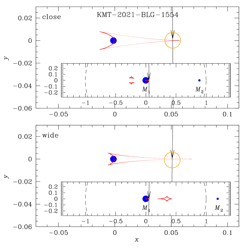
Detailed analysis of the light curve indicates that the anomaly was produced by a planetary companion to the lens. We find two sets of solutions with planet parameters of and resulting from the close-wide degeneracy. The full lensing parameters of both solutions are provided in Table 6. It is found that the degeneracy between the two 2L1S solution is severe with , and the 2L1S solutions are favored over the model under the 1L2S interpretation by . The lensing parameters of the 1L2S model are listed in Table 6. We compare the residuals of the 2L1S and 1L2S models in the two middle panels of Figure 8. It turns out that the source crossed a caustic, and thus we are able to measure the normalized source radius, .
The lensing configurations of the event according to the close and wide solutions are shown in the upper and lower panels of Figure 9, respectively. The figure shows that the anomaly was produced by the crossing of the source over the sharp tip of the central caustic induced by a planet lying near the Einstein ring of the planet host. The gap between the caustic entrance and exit is much smaller than the source size, and thus the individual caustic-crossing features do not show up in the anomaly and instead the anomaly appears as a single bump. The incidence angle of the source on the binary axis is nearly , and thus the features on the rising and falling sides of the anomaly are symmetric.
4 Source stars and angular Einstein radii
Among the four analyzed planetary events, the anomalies of the three events (KMT-2017-BLG-0752, KMT-2021-BLG-1303, and KMT-2021-BLG-1554) were affected by finite-source effects, and thus the normalized source radii can be measured. In this section, we estimate the angular Einstein radii for these events. Estimating from a measured value requires one to specify the source type, from which the angular source radius is deduced and the Einstein radius is determined by
| (3) |
Although the normalized source radius and thus cannot be measured for the event KMT-2021-BLG-0320, we specify the source type for the sake of completeness.
The specification of the source type is done by estimating the color and brightness of the source. We measure the and -band magnitudes of the source from the regression of the data processed using the pyDIA photometry code (Albrow, 2017) with the variation of the lensing magnification. We then place the source on the instrumental color-magnitude diagram (CMD) of stars lying around the source constructed using the same photometry code. Following the method of Yoo et al. (2004), the instrumental source color and magnitude, , are then calibrated using the centroid of red giant clump (RGC), for which its reddening and extinction-corrected (de-reddened) color and magnitude, , are known, on the CMD as a reference.
Figure 10 shows the positions of the source stars (marked by blue dots) with respect to those of the RGC centroids (red dots) on the CMDs of the individual events. For OGLE-2017-BLG-1691, the source color could not be securely measured not only because the -band data sparsely covered the light curve during the lensing magnification but also because the photometry quality of these data is low, although the -band magnitude was relatively well measured. In this case, we estimated the source color as the median color of stars with the same -band magnitude offset from the RGC centroid in the CMD constructed from the images of Baade’s window taken from the observations using the Hubble Space Telescope (Holtzman et al., 1998). From the offsets in color and magnitudes between the source and RGC centroid, , together with the known de-reddened color and magnitude of the RGC centroid, (Bensby et al., 2013; Nataf et al., 2013), we estimate the calibrated source color and magnitude as . In Table 7, we list the source colors and magnitudes of the individual events estimated from this procedure along with the spectral types of the source stars. It is found that the source of OGLE-2017-BLG-1691 is a turnoff star or a subgiant of a G spectral type, while the source stars of the other events are main-sequence stars with spectral types ranging from G to K.

For each event, the angular source radius and Einstein radius were estimated from the measured color and magnitude of the source. For this, the measured color was converted into color using the color-color relation of Bessell & Brett (1988), value was interpolated from the ()– relation of Kervella et al. (2004), and then the angular Einstein radius was estimated using the relation in Equation (3). With the measured Einstein radius together with the event time scale, the value of the relative lens-source proper motion was assessed as
| (4) |
In Table 8, we list the estimated values of , , and for the individual events. The and values for the event KMT-2021-BLG-0320 are left blank because finite-source effects in the lensing light curve were not detected and subsequently the values of , , and could not be measured. We note that the angular Einstein radius of KMT-2021-BLG-1554, mas, is substantially smaller than those of the other events, and this together with its short time scale, days, suggests that the mass of the lens would be very low. KMT-2021-BLG-1554 is the seventh shortest microlensing event with a bound planet. See Table 3 of Ryu et al. (2021).
| Event | () | () | (kpc) | (AU) |
|---|---|---|---|---|
| OGLE-2017-BLG-1691 | (inner) | |||
| – | – | – | (outer) | |
| KMT-2021-BLG-0320 | (close) | |||
| – | – | – | (wide) | |
| KMT-2021-BLG-1303 | ||||
| KMT-2021-BLG-1554 | (close) | |||
| – | – | – | (wide) |
5 Physical parameters
In this section, we estimate the physical parameters of the planetary systems. For the unique constraint of the physical lens parameters, one must simultaneously measure the extra observables of and , from which the mass and distance to the lens, , are determined as
| (5) |
Here , , and denotes the distance to the source (Gould, 1992, 2000). The values of the microlens parallax could not be measured for any of the events, and thus the physical parameters cannot be unambiguously determined from the relation in Equation (5). However, one can still constrain and using the other measured observables of and , which are related to the physical lens parameters as
| (6) |
where denotes the relative parallax between the lens and source. The event time scales were well measured for all events, and the Einstein radii were assessed for three of the four events. In order to estimate the physical lens parameters with the constraints provided by the measured observables of the individual events, we conduct Bayesian analyses using a Galactic model.

In the Bayesian analysis, we started by producing many lensing events from a Monte Carlo simulation conducted with the use of a Galactic model, which defines the matter-density and kinetic distributions, and mass function of Galactic objects. We adopted the Galactic model constructed by Jung et al. (2021). In this model, the density distributions of disk and bulge objects are described by the Robin et al. (2003) and Han & Gould (2003) models, respectively. The kinematic distribution of disk objects is based on the modified version of the Han & Gould (1995) model, in which the original version is modified to reconcile the changed density model, that is, the Robin et al. (2003) model. The bulge kinematic distribution is modeled based on proper motions of stars in the Gaia catalog (Gaia Collaboration, 2016, 2018). For the details of the density and kinematic distributions, see Jung et al. (2021). In the Galactic model, the mass function is constructed with the adoption of the initial mass function and the present-day mass function of Chabrier (2003) for the bulge and disk lens populations, respectively.

In the second step, we computed the time scales and Einstein radii of the simulated events using the relations in Equation (6), and then constructed posterior distributions of and for the simulated events with the and values that are consistent with the observables of the individual lensing events. For the three events OGLE-2017-BLG-1691, KMT-2021-BLG-1303, and KMT-2021-BLG-1554, we use the constraints of both and , and for KMT-2021-BLG-0320, we apply the constraint of only because is not measured for the event.
Figures 11 and 12 show the Bayesian posteriors of and of the individual events, respectively. In Table 9, we summarize the estimated values of the host and planet masses, and , distance, and projected host-planet separation, , for all of which medians are presented as representative values and the uncertainties are estimated as 16% and 84% of the Bayesian posterior distributions. The median values and uncertainty ranges of the individual events are marked by solid and dotted vertical lines in the Bayesian posteriors presented in Figures 11 and 12, respectively. For the events with degenerate solutions, OGLE-2017-BLG-1691, KMT-2021-BLG-0320 and KMT-2021-BLG-1554, we present the planetary separations corresponding to both the close and wide (or inner and outer) solutions. We note that the uncertainties of the estimated physical parameters are big because of the intrinsically weak Bayesian constraint. For example, from the comparison of the posterior distributions of OGLE-2017-BLG-1691 and KMT-2021-BLG-0320, one finds that the difference between the two posterior distributions is not significant, although the mean lens mass for the former event is slightly bigger than that of the latter event due to the longer time scale and the uncertainty is smaller due to the additional constrain of .
The estimated masses indicate that all of the discovered planets have sub-Jovian masses. The planet masses KMT-2021-BLG-0320L, KMT-2021-BLG-1303L, and KMT-2021-BLG-1554L correspond to , , and times of the mass of the Jupiter, and the planet mass of OGLE-2017-BLG-1691L corresponds to that of Uranus. To be noted among the planet hosts is that the estimated mass of the planetary system KMT-2021-BLG-1554L, , corresponds to the boundary between a star and a brown dwarf (BD). Together with the previously detected planetary systems with very low-mass hosts444MOA-2011-BLG-262 (Bennett et al., 2014), OGLE-2012-BLG-0358 (Han et al., 2013), MOA-2015-BLG-337 (Miyazaki et al., 2018), OGLE-2015-BLG-1771 (Zhang et al., 2020), KMT-2016-BLG-1820 (Jung et al., 2018a), KMT-2016-BLG-2605 (Ryu et al., 2021), OGLE-2017-BLG-1522 (Jung et al., 2018b), OGLE-2018-BLG-0677 (Herrera-Martín et al., 2020), KMT-2018-BLG-0748 (Han et al., 2020b), and KMT-2019-BLG-1339L (Han et al., 2020a), the discovery of the system demonstrates the microlensing capability of detecting planetary systems with very faint or substellar hosts. Besides KMT-2021-BLG-1554L, the host stars of the other planetary systems are low-mass stars with masses lying in the range of –. Under the approximation that the snow line distance scales with the host mass as AU, all discovered planets lie beyond the snow lines of the hosts regardless of the solutions, demonstrating the high microlensing sensitivity to cold planets. The planetary systems lie in the distance range of – kpc, demonstrating the usefulness of the microlensing method in detecting remote planets.
6 Summary and conclusion
We presented the analyses of four planetary microlensing events OGLE-2017-BLG-1691, KMT-2021-BLG-0320, KMT-2021-BLG-1303, and KMT-2021-BLG-1554. The events share a common characteristic that the planetary signals appeared as anomalies with very short durations, ranging from a few hours to a couple of days, and they were clearly detected solely by the combined data of the high-cadence lensing surveys without additional data from followup observations.
From the detailed analyses of the events, it was found that the signals were generated by planets with low planet-to-host mass ratios: three of the planetary systems with mass ratios of the order of and the other with a mass ratio slightly greater than . In the histogram of microlensing planets presented in Figure 1, we mark the positions of the four planets discovered in this work. The estimated masses indicated that all discovered planets have sub-Jovian masses, in which the planet masses of KMT-2021-BLG-0320Lb, KMT-2021-BLG-1303Lb, and KMT-2021-BLG-1554Lb correspond to , , and times of the mass of the Jupiter, and the mass of OGLE-2017-BLG-1691Lb corresponds to that of the Uranus. It was found that the host of the planetary system KMT-2021-BLG-1554L has a mass at around the boundary between a star and a brown dwarf. Besides this system, it was found that the host stars of the other planetary systems are low-mass stars with masses in the range of –. The discoveries of the planets well demonstrate the capability of the current high-cadence microlensing surveys in detecting low-mass planets.
Acknowledgements.
Work by C.H. was supported by the grants of National Research Foundation of Korea (2020R1A4A2002885 and 2019R1A2C2085965). This research has made use of the KMTNet system operated by the Korea Astronomy and Space Science Institute (KASI) and the data were obtained at three host sites of CTIO in Chile, SAAO in South Africa, and SSO in Australia. The OGLE project has received funding from the National Science Centre, Poland, grant MAESTRO 2014/14/A/ST9/00121 to AU. he MOA project is supported by JSPS KAKENHI grant Nos. JSPS24253004, JSPS26247023, JSPS23340064, JSPS15H00781, JP16H06287, JP17H02871, and JP19KK0082.References
- Alard & Lupton (1998) Alard, C., & Lupton, R. H. 1998, ApJ, 503, 325
- Albrow (2017) Albrow, M. 2017, MichaelDAlbrow/pyDIA: Initial Release on Github,Versionv1.0.0, Zenodo, doi:10.5281/zenodo.268049
- Albrow et al. (2009) Albrow, M., Horne, K., Bramich, D. M., et al. 2009, MNRAS, 397, 2099
- An (2005) An, J. H. 2005, MNRAS, 356, 1409
- Bennett et al. (2014) Bennett, D. P., Batista, V., Bond, I. A., et al. 2014, ApJ, 785, 155
- Bennett & Rhie (1996) Bennett, D. P., & Rhie, S. H. 1996, ApJ, 472, 660
- Bensby et al. (2013) Bensby, T., Yee, J. C., Feltzing, S., et al. 2013, A&A, 549, A147
- Bessell & Brett (1988) Bessell, M. S., & Brett, J. M. 1988, PASP, 100, 1134
- Bond et al. (2001) Bond, I. A., Abe, F., Dodd, R. J., et al. 2001, MNRAS, 327, 868
- Chabrier (2003) Chabrier, G. 2003, PASP, 115, 763
- Dominik (1999) Dominik, M. 1999, A&A, 349, 108
- Dominik (2019) Dominik, M., Bachelet, E., Bozza, V., et al. 2019, MNRAS, 484, 5608
- Gaia Collaboration (2016) Gaia Collaboration, Prusti, T., de Bruijne, J. H. J., et al. 2016, A&A, 595, A1
- Gaia Collaboration (2018) Gaia Collaboration, Brown, A. G. A., Vallenari, A., et al. 2018, A&A, 616, A1
- Gaudi (1998) Gaudi, B. S. 1998, ApJ, 506, 533
- Gaudi & Gould (1997) Gaudi, B. S., & Gould, A. 1997, ApJ, 486, 85
- Gould (1992) Gould, A. 1992, ApJ, 392, 442
- Gould & Loeb (1992) Gould, A., & Loeb, A. 1992, ApJ, 396, 104
- Gould (2000) Gould, A. 2000, ApJ, 542, 785
- Griest & Safizadeh (1998) Griest, K., & Safizadeh, N. 1998, ApJ, 500, 37
- Han et al. (2022a) Han, C. Bond, I. A., Yee, J. C., et al. 2022a, A&A, 658, A62
- Han & Gould (1995) Han, C., & Gould, A. 1995, ApJ, 447, 53
- Han & Gould (2003) Han, C., & Gould, A. 2003, ApJ, 592, 172
- Han et al. (2022b) Han, C., Gould, A., Albrow, M. D., et al. 2022b, A&A, 658, A94
- Han et al. (2013) Han, C., Jung, Y. K., Udalski, A., et al. 2013, ApJ, 778, 38
- Han et al. (2020a) Han, C., Kim, D., Udalski, A., et al. 2020a, AJ, 160, 64
- Han et al. (2020b) Han, C., Shin, I.-G., Jung, Y. K., et al. 2020b, A&A, 641, A105
- Han et al. (2021) Han, C., Udalski, A., Kim, D., et al. 2021, A&A, 655, A21
- Han et al. (2022c) Han, C., Udalski, A., Lee, C.-U., et al. 2022c, A&A, 658, A93
- Herrera-Martín et al. (2020) Herrera-Martín, A., Albrow, A., Udalski, A., et al. 2020, AJ, 159, 134
- Holtzman et al. (1998) Holtzman, J. A., Watson, A. M., Baum, W. A., Grillmair, C. J., Groth, E. J., Light, R. M., Lynds, R., & O’Neil, E. J.,Jr. 1998, AJ, 115, 1946
- Hwang et al. (2022) Hwang, K.-H., Zang, W., Gould, A., et al. 2022, AJ, 163, 43
- Jung et al. (2021) Jung, Y. K., Han, C., Udalski, A., et al. 2021, AJ, 161, 293
- Jung et al. (2018a) Jung, Y. K., Hwang, K.-H., Ryu, Y.-H., et al. 2018a, AJ, 156, 208
- Jung et al. (2018b) Jung, Y. K., Udalski, A., Gould, A., et al. 2018b, AJ, 155, 219
- Kervella et al. (2004) Kervella, P., Thévenin, F., Di Folco, E., & Ségransan, D. 2004, A&A, 426, 29
- Kim et al. (2018) Kim, D.-J., Kim, H.-W., Hwang, K.-H., et al. 2018, AJ, 155, 76
- Kim et al. (2016) Kim, S.-L., Lee, C.-U., Park, B.-G., et al. 2016, JKAS, 49, 37
- Miyazaki et al. (2018) Miyazaki, S., Sumi, T., Bennett, D. P., et al. 2018, AJ, 156, 136
- Nataf et al. (2013) Nataf, D. M., Gould, A., Fouqué, P., et al. 2013, ApJ, 769, 88
- Robin et al. (2003) Robin, A. C., Reylé, C., Derriére, S., & Picaud, S. 2003, A&A, 409, 523
- Ryu et al. (2021) Ryu, Y. H., Hwang, K.-H., Gould, A., et al. 2021, AJ, 162, 96.
- Ryu et al. (2022) Ryu, Y. H., Jung Y. K., Yang, H., et al. 2022, in preparation
- Shin et al. (2022) Shin, I.-G., Yee, J. C., Hwang K.-H., et al. 2022, AJ, in press (arXiv:2201.04312)
- Tomaney & Crotts (1996) Tomaney, A. B., & Crotts, A. P. S. 1996, AJ, 112, 2872
- Udalski et al. (2015) Udalski, A., Szymański, M. K., & Szymański, G. 2015, Acta Astron., 65, 1
- Woźniak (2000) Woźniak, P. R. 2000, Acta Astron., 50, 42
- Yee et al. (2012) Yee, J. C., Shvartzvald, Y., Gal-Yam, A., et al. 2012, ApJ, 755, 102
- Yee et al. (2021) Yee, J. C., Zang, W, Udalski, A., et al. 2021, AJ, 162, 180
- Yoo et al. (2004) Yoo, J., DePoy, D. L., Gal-Yam, A., et al. 2004, ApJ, 603, 139
- Zang et al. (2021a) Zang, W., Han, C., Kondo, I., et al. 2021, Rearcxh in Astron and Astroph., 2021a, 21, 239
- Zang et al. (2021b) Zang, W., Hwang, K.-H., Udalski, A., et al. 2021b, AJ, 162, 163
- Zhang et al. (2022) Zhang, K., Gaudi, B. S., & Bloom, J. S. 2022, Nature Astronomy, submitted, arXiv:2111.13696
- Zhang et al. (2020) Zhang, X., Zang, W., Udalski, A., et al. 2020, AJ, 159, 116