Fourth order real space solver for the time-dependent Schrödinger equation with singular Coulomb potential
Abstract
We present a novel numerical method and algorithm for the solution of the 3D axially symmetric time-dependent Schrödinger equation in cylindrical coordinates, involving singular Coulomb potential terms besides a smooth time-dependent potential. We use fourth order finite difference real space discretization, with special formulae for the arising Neumann and Robin boundary conditions along the symmetry axis. Our propagation algorithm is based on merging the method of the split-operator approximation of the exponential operator with the implicit equations of second order cylindrical 2D Crank-Nicolson scheme. We call this method hybrid splitting scheme because it inherits both the speed of the split step finite difference schemes and the robustness of the full Crank-Nicolson scheme. Based on a thorough error analysis, we verified both the fourth order accuracy of the spatial discretization in the optimal spatial step size range, and the fourth order scaling with the time step in the case of proper high order expressions of the split-operator. We demonstrate the performance and high accuracy of our hybrid splitting scheme by simulating optical tunneling from a hydrogen atom due to a few-cycle laser pulse with linear polarization.
keywords:
Time-dependent Schrödinger equation , Singular Coulomb potential , High order methods , Operator splitting , Crank-Nicolson scheme , Strong field physics , Optical tunneling1 Introduction
Experiments with attosecond light pulses [1, 2, 3, 4, 5, 6], based on high-order harmonic generation (HHG) in noble gases [7, 8, 9, 10], have been revolutionizing our view of fundamental atomic, molecular and solid state processes in this time domain [11, 12, 13, 14, 15, 16, 17]. A key step in gas-HHG is the tunnel ionization of a single atom and the return of the just liberated electron to its parent ion [18, 19], due to the strong, linearly polarized femtosecond laser pulse driving this process. Recent developments in attosecond physics revealed that the accurate description of this single-atom emission is more important than ever, e.g. for the correct interpretation of the data measured in attosecond metrology experiments, especially regarding the problem of the zero of time [20, 15], and the problem of the exit momentum [13]. Although an intuitive and very successful approximate analytical solution [21] and many of its refinements exist [22], the most accurate description of the single-atom response is given by the numerical solution of the time-dependent Schrödinger equation (TDSE).
The common model of the single-atom response employs the single active electron approximation and the dipole approximation. These reduce the problem to the motion of an electron in the time-dependent potential formed by adding the effect of the time-dependent electric field to the atomic binding potential. The peculiarity of this problem is due to the strength of the electric field, which has its maximum typically in the range of 0.05-0.1 atomic units. Thus, this electric field enables the tunneling of the electron through the (time-dependent) potential barrier formed by strongly distorting the atomic potential, but this effect is weak during the whole process. On the other hand, this small part of the wave function outside the barrier extends to large distances and in fact this is the main contribution to the time-dependent dipole moment, which is usually considered as the source of the emitted radiation. Thus, a very weak effect needs to be computed very accurately, and these requirements get even more severe, if the model goes beyond the single active electron or the dipole approximation.
The fundamental importance of the singularity of the Coulomb potential regarding HHG has already been analysed and emphasized e.g. in [23]. As other kind of numerical errors decrease, the artifacts caused by the smoothing of the singularity become more disturbing. Therefore, a high precision numerical method has to handle the Coulomb singularity as accurately and effectively as possible.
The most widely employed approach to the numerical solution of the TDSE for an atomic electron driven by a strong laser pulse is to use spherical polar coordinates: then the hydrogen eigenfunctions are analytic and one expands the wavefunction in spherical harmonics with expansion coefficients acting as radial or reduced radial functions, for which the problem is solved directly. For example, these radial functions can be further expanded using a suitable basis, like Gaussian-Legendre or B-splines [24, 25, 26], in which the Hamiltonian matrix does not have any singularity. Also, refined solutions based on highly accurate real space discretization of the radial coordinate exist using this harmonic expansion [27, 28, 29, 30, 31], also relying on the fact that a boundary condition for can be derived from the analytic properties of hydrogenic eigenfunctions and can be built into the implicit equations. The usual drawback is that in order to calculate physical quantities either the real space reconstruction of the wavefunction is necessary or every observable must be given in this harmonic expansion. Also, the spherical grid of these methods is not well adapted to the electron’s motion which is mainly along the polarization direction of the laser field.
One can easily stumble upon applications other than HHG where neither spherical coordinates, nor special basis functions are optimal, and one has to use Cartesian or cylindrical coordinate systems in numerical simulations, and of course, discretization of real space coordinates. The most basic method is just to use a staggered grid which avoids the singularity of the Coulomb potential [32]: then the scheme will be easily solvable, although with low accuracy. A somewhat refined version of this is using a smoothed version of the potential, for example the so called soft Coulomb-form of , where the value of can be fitted by matching the ground state energy with that of the true hydrogen atom [32, 33, 34, 35]. These approximations are rather crude, but can reproduce important features of the quantum system [23]. Recently, Gordon et. al. [36] provided an improved way to include the Coulomb singularity, by using the general asymptotic behavior of the hydrogen eigenstates around . They built an improved discrete Hamiltonian matrix through a new discrete potential, using a three point finite difference scheme. This way they increased the accuracy of the numerical solution by an order of magnitude.
In the present work, we propose a novel method to accurately incorporate the effect of the Coulomb singularity in the solution of a spinless, axially symmetric TDSE, in cylindrical coordinates. We account for the singular Coulomb potential through analytic boundary condition which resolves the problem of nondifferentiability of the hydrogen eigenfunctions in the cylindrical coordinate system and yields high order spatial accuracy.
Incorporating this kind of analytic boundary condition into the numerical solution of TDSE will constrain the applicable propagation methods because the singularity of the Coulomb potential at and the singularity of the cylindrical radial coordinate at will introduce Robin and Neumann boundary conditions, overriding the Hamilton operator. As a consequence, typical explicit methods, for example staggered leapfrog [36, 37], second order symmetric difference method [38, 39], any polynomial expansion method [38, 40], and split-step Fourier transformation methods [38, 41, 42] have been ruled out, leaving only implicit methods.
In Section 2, we introduce the cylindrical TDSE to be solved, along with its boundary conditions, and we describe the way how we incorporate the singular Coulomb potential to the problem. In Section 3, we derive the suitable finite-difference scheme with high order spatial accuracy, using second order Crank-Nicolson method [38, 43, 44]. We briefly go through the standard approximations of the evolution operator, then we write down the detailed form of the resulting implicit linear equations. In Section 4, we overview the standard split-operator methods for numerically solving the TDSE, and combine them with the finite-difference description, which is known as split-step finite difference method [45, 46]. We show that similarly to the typical explicit methods, real space split-operator methods do not work well for singular Hamiltonians. Based in these conclusions, we introduce our hybrid splitting method, which retains the robustness of the full Crank-Nicolson method and the speed of the split-operator method. In Section 5, we analyse the newly arisen coefficient matrix, we describe the way how to take advantage of its structure, then we derive a special solver algorithm which is necessary for fast solution of the TDSE. In Section 6, we discuss the results of numerical experiments we carried out with our hybrid splitting method: (i) for the accuracy of the spatial discretization of the finite difference scheme, we calculate the eigenenergies of selected eigenstates, (ii) for the temporal accuracy of our split-step finite difference scheme combined with high order evolution operator factorizations, we compare the numerical wave function with the analytic solution of the quantum forced harmonic oscillator, (iii) for final verification, we simulate the hydrogen atom in a time dependent external electric field.
2 Schrödinger equation and boundary conditions
2.1 The time-dependent Schrödinger equation
Let us consider the axially symmetric three-dimensional time-dependent Schrödinger equation in cylindrical coordinates and :
| (1) |
where is the (reduced) electron mass. For the sake of simplicity, we use atomic units throughout this article and we use the notation .
As discussed in the Introduction, such a Hamiltonian plays a fundamental role e.g. in the interaction of atomic systems with strong laser pulses. Then the potential is usually the sum of an atomic binding potential (centered in the origin) and an interaction energy term. For a single active electron and a linearly polarized laser pulse, this interaction term in dipole approximation and in length gauge [47] reads as:
| (2) |
where denotes the electron’s electric charge and is the laser’s electric field, pointing in the direction.
The wave function is defined within the interval , and the problem is treated as an initial value problem as is known. Box boundary conditions are posed at three edges of the interval:
| (3) |
and because of the singularity in the curvilinear coordinate , Neumann boundary condition should be posed along the line . In order to find this boundary condition, we multiply (1) by and take the limit :
| (4) |
where we have assumed the potential is smooth at line. Then is continuous and continuously differentiable everywhere in the plane, and it has extremal value in . Symmetry condition also holds in this case.
However, this Neumann boundary condition has to be altered when we introduce a singular potential in any form, e.g. the 3D Coulomb potential with and .
2.2 The boundary condition for the 3D Coulomb potential
Our aim is to represent the singularity of the 3D Coulomb potential by implementing the correct boundary condition in the origin. In order to find this condition, it seems necessary to use spherical polar coordinates, since the Coulomb problem is not separable in cylindrical coordinates. Let us first discuss the properties of the radial solutions of the well known radial equation [48, 49]:
| (5) |
where is the angular momentum quantum number. If we multiply both sides with then take the limit, we can acquire Robin boundary condition for all of the states as
| (6) |
but the bound states with higher angular momenta will have boundary condition at the origin, in accordance with the fact that for the particle physically cannot penetrate to , because of the singularity of .
Since we need the boundary conditions for the cylindrical equation independent of the values, we turn to the nonseparated symmetric spherical Schrödinger equation for answers:
| (7) |
which has also the term and has singularity at and at , . To acquire the boundary conditions for , we again multiply both sides with and take the limit, yielding
| (8) |
Now we transform equation (8) into cylindrical coordinates and , using following expressions of the partial derivatives:
| (9) |
| (10) |
with and . After writing back and taking the limit, the formula (8) becomes
| (11) |
Then, by substituting into (11), we obtain the Robin boundary condition for the 3D Coulomb singularity:
| (12) |
This can be generalized to include multiple Coulomb-cores rather easily, we just need to impose (12) at multiple points along the axis. Additionally, any continuously differentiable potential added to this configuration does not change this boundary condition. It is interesting to note also that the boundary condition imposed by a 1D Dirac-delta potential also has the form of (12) for a symmetric wave function [49].
2.3 The states with nonzero magnetic quantum numbers
Although we are mainly interested in the solution of the TDSE with an axially symmetric initial state, i.e. an initial state of zero magnetic quantum number , we briefly show in the following that initial states with nonzero also lead to a TDSE of the form (13), however with different boundary conditions at .
Let us write out the full 3D cylindrical time-dependent Schrödinger equation, again with the same axially symmetric potential that we used previously:
| (13) |
We can write the quantum state with a given magnetic quantum number in the following form for any
| (14) |
due to the fact that the Hamiltonian of (13) conserves the quantum number. (We can also use real angular basis functions like or instead of , as long as that they are the eigenfunctions of .)
After substituting (14) to (13) we perform projection in the form of . Then we get the TDSE for our wave function with the specified magnetic quantum number :
| (15) |
Eq. (15) has the same form as the axially symmetric equation (1) but with a new dependent potential:
| (16) |
However, if then the singularity of (16) alters the boundary condition (4) at the axis to the following:
| (17) |
which can by derived by multiplying (15) with and taking the limit of . The boundary condition (17) also works with Coulomb potential, and in every case where in the limit of . It is also consistent with the boundary conditions for Coulomb states with nonzero angular momenta () mentioned in the previous section.
3 The Crank-Nicolson method
3.1 Approximation of the time evolution operator
The formal solution of (1) in terms of the time evolution operator is the following
| (18) |
Here, the exponential operator is to be understood as a time-ordered quantity, which is a difficult procedure if the Hamilton operators at different time instants do not commute. However, this is the case for the potential we are considering.
To acquire suitable discretization in the time domain of problem (1) we approximate the time evolution operator directly. First, let us divide the time domain , into equal subintervals, then by the group property of we get
| (19) |
where and . In one interval, we can write the evolution operator with its short time form of
| (20) |
where is the effective time-independent Hamiltonian related to the original one by the Magnus expansion [50, 51]:
| (21) |
This includes infinitely many commutators of the Hamiltonians evaluated at different time points, to be integrated with respect to more and more variables.
Using only the first term of this series, one can directly acquire the well known second order approximation of the Hamiltonian as
| (22) |
In order to have information about the next error term of the time evolution, we need to evaluate the Magnus commutator series to fourth order. According to Puzynin et. al. [50], this improved approximation for a TDSE of the form (1) is
| (23) |
where the top dots are the short hand notation for time derivatives. This formula is important even if we use only the second order approximation, because the leading order of error depends on characteristics of the first and second time derivatives of .
For the exponential operators (20), first we consider the diagonal Padé-approximation of an exponential function
| (24) |
where is the confluent hypergeometric function, which in this case reduces to a polynomial of degree with real coefficients. This expression can be used for the exponential operators (20) with , and it can be shown that for self-adjoint operators the approximation is unitary [23].
From this, a generalized operator approximation scheme that is accurate can be obtained [44, 52] in a general form of
| (25) |
where for are the roots of the polynomial equation
| (26) |
If we truncate both the Magnus-series at the first term in (21) and take a single coefficient of the Padé-approximation (), then we arrive at the second order accurate implicit Crank-Nicolson scheme:
| (27) |
One can straightforwardly construct higher order Crank-Nicolson schemes using (25), yielding multiple implicit Crank-Nicolson substeps [44]. For time dependent Hamiltonians though, a high order accurate scheme should use the corresponding high order effective Hamiltonian (21) for consistency.
3.2 The finite difference scheme
Our next step is to discretize the effective Hamiltonian , and to construct the Hamiltonian matrix. We propose to use the method of fourth order finite differences with cylindrical coordinates and the following equidistant 2D spatial grid:
| (28) |
| (29) |
The first term of the Hamiltonian is the Laplacian . We denote the finite difference approximation of its - and -dependent terms by and , respectively, and we use the following fourth order accurate finite difference forms [52] for them:
| (30) |
| (31) |
These fourth order formulae are optimal in the sense that symmetric finite differences of more than five points are very complicated to be applied for the Coulomb-problem, because the higher order the finite difference formula is, the higher derivatives of should be continuous.
To discretize the Neumann and Robin boundary conditions, we need a one-sided finite difference formula for the first derivative. Based on the method of Ref. [52], we derived the following fourth order accurate forward difference operator:
| (32) |
Using standard second order accurate form (27) of the exponential operator with the discretized Laplacian in the Hamilton matrix, we get the following implicit scheme for all and :
| (33) |
where and the potential is evaluated at the temporal midpoint . The box boundary conditions is applied if or or .
Assuming that the potential is smooth, the Neumann boundary condition (4) prescribes the following implicit equations at for all :
| (34) |
On the other hand, if a Coulomb-core of strength is present at the grid point and then, according to (12), equation (34) will be overridden at by
| (35) |
Here we have assumed that the origin is included in (28) with , where can be anywhere in the interval if it is reasonably far from the box boundaries.
For states, the equations of the boundary conditions at are simply with or without Coulomb potential.
For simplicity, let us introduce the short hand notations , then by substituting the finite difference Laplacians (30), (31) into (33), we arrive at the following final form of linear equations for all , :
| (36) |
where
| (37) |
For the configuration, the equations forced by the Neumann and Robin boundary conditions for all from (32), (34), (35) are
| (38) |
For the states we have simply
| (39) |
The spatial discretization in the cylindrical coordinate system and the Neumann or Robin boundary conditions for the states make the unitarity of the algorithm, and in a broader sense, the accuracy of spatial integrations a more subtle issue than usual. One has to find an appropriate discrete inner product formula that is conserved at least with the accuracy of the finite differences, and which can be evaluated with sufficient accuracy using the cylindrical grid. We give a solution to this auxiliary problem in A.
Although it corresponds to 3D propagation, we call this scheme 2D Crank-Nicolson method because it involves only two spatial coordinates. This is already a complete propagation algorithm by itself, however, it suffers from the numerically inefficient solution of the resulting linear equations: if we combine the indices into a single one (by flattening the two dimensional array) as , we obtain a a block pentadiagonal matrix of size , with block size . Inverting this type of matrix is computationally intense [43, 53] because the width of the diagonal is : despite its apparent simplicity, the numerical cost of this task is which is extremely high compared to the cost of a pentadiagonal scheme of the same size. These facts inspired us to develop an improved algorithm which has almost all advantages of this 2D Crank-Nicolson method but needs much less numerical effort.
4 Operator splitting schemes
As we have seen in the previous section, the 2D Crank-Nicolson scheme with the boundary condition (4) is a possible but ineffective way of solving the TDSE numerically. Now we are going to discuss how to apply the well-known method of operator splitting to the solution of the problem described in the introduction.
4.1 Operator splitting formulae
The approach of the operator splitting method is to factorize the exponential operator into multiple easy-to-solve parts. From the Taylor-expansion of the exponential operator
| (40) |
follow the two main formulae [54] which form the basis of the operator splitting schemes, namely the Baker-Campbell-Hausdorff formula :
| (41) |
and the Zassenhaus formula
| (42) |
Both of these contain infinitely many commutators of and . Of course, if then exactly. As the above formulae suggest, the terms can be further factorized into the exponents. An extended analysis is available in Refs. [55, 56].
If one uses (41) and (42) to acquire a symmetric decomposition, only odd leading order of will appear in the formula. This is a requirement for quantum propagation though, because the presence of even order terms would destroy the unitary evolution of the wave function. A well-known example of this is the widely used standard symmetric second order accurate formula (or Strang splitting, after [57]):
| (43) |
where is a combination of commutators of and . A direct fourth order splitting scheme was derived by Chin and Suzuki [58, 59]:
| (44) |
This splitting requires also the evaluation of the commutator, which can rise additional difficulties, depending on the particular form of and .
We proceed by introducing another kind of higher order operator splitting, based on the work of Bandrauk and Shen [60], who developed an iterative method to improve the accuracy of the (43) scheme. Let us denote the second order accurate form with , then their iteration method reads for as
| (45) |
where the parameter must be for each iteration step a real root of the corresponding polynomial equation
| (46) |
In (45) only the odd error terms appear, because of the unitarity and the symmetry of the splitting scheme. So the requires evaluations of , in the worst case. For completeness we note, that using the complex roots of (46) in (45) is also a viable approach in some numerical applications [59, 61].
This scheme was already generalized for time-dependent Hamiltonians of the form in [60, 62] as follows. Inserting the second order effective Hamiltonian (22) into the formula (43) with , the second order accurate splitting of the evolution operator becomes
| (47) |
Then (45) will take the form for
| (48) |
and being the same as in the time-independent case (46). Interestingly, the fourth order approximation in (48) decreases the error even if the time evolution governed by a nonlinear time-dependent Schrödinger equations, if the nonlinear error term is corrected in the formulation of the propagator [62, 61].
Now we write out a new form of iteration (48) for time-dependent Hamiltonians, by using the same principles, for
| (49) |
where , must be the simultaneous real roots of equations
| (50) |
However, this formula for requires five evaluations of , compared to nine in the case of the (45).
Although the fourth order formula (44) with the fourth order effective Hamiltonian (23) seems to be superior compared to the iterative propagation (48) (because of the extra information given by the temporal and spatial commutators, and less evaluations), the schemes (48) and (49) do not require the calculation of commutators, they decrease all the dependent errors simultaneously and they are easy to implement. However, they involve backward time steps, which means they do not work very well with diffusive problems.
Another class of high order split-operator methods for diffusive partial differential equations was developed in [63], where the exponential operator is found by an ansatz of
| (51) |
Here is the same second order formula which is used in (45). The fourth order formula is simply given by . Thus, once is properly constructed, all high order formulae (48), (49), (51) can be utilized immediately. The (51) method is suitable for the imaginary time propagation [28, 63, 64] with , i.e. for determination of the lowest energy eigenstates of stationary potentials.
A problem also arises when one wishes to use an imaginary potential [65] with (48) and (49), which is a commonly used numerical technique to avoid artificial reflections from the (box) boundaries of the simulation domain. Adding an imaginary potential into the Hamiltonian gives the following splitting of the exponential operator from (43):
| (52) |
It is clear that performs the required absorption of the wavefunction in the case of forward time propagation , but it would blow up the wave function during the necessary backward steps in (48) and (49). We circumvented this problem by partially disallowing backward steps, i.e. we replaced by .
4.2 Directional splitting of the exponential operator
The most common way of factorizing the exponential operator is that the different spatial coordinate derivatives decouple into different exponential operators, i.e. to use a directional splitting. Then the propagation can be carried out by solving multiple one dimensional TDSE-s in succession. The most frequent realization of this is the so-called potential-kinetic term splitting, which is mainly used in conjunction with the Fourier-transformation methods in Cartesian coordinates [38, 41, 42]. However, if we apply the potential-kinetic term splitting to problem of (1) then we have to write Hamiltonian as where is the potential, and are the kinetic energy operators. The commutator will take a rather simple form of . Thus, the direct second order (43) and fourth order (44) symmetric splitting schemes are written as
| (53) |
| (54) |
where . We also note that these split-operator formulae by themself will introduce error, scaling as and , compared to the stationary states of the exact time-independent Hamiltonian. In the case of a time-dependent Hamiltonian, the respective second order (22) or fourth order (23) effective Hamiltonians should be used. These truncations of the Magnus-series (21) will introduce additional and dependent errors in time evolution.
The magnitudes of the aforementioned numerical errors will depend on the derivatives of : in the case of an external electric field the smoothness of in time is a reasonable assumption. On the other hand, the spatial dependence of the atomic potential should also behave the same way if we wish to use operator splitting. As we suspect, it will not always be the case, especially in atomic or molecular physics. We can deduce from (54) that the leading order of error of the second order scheme must have a dependence of , e.g. the error characteristics strongly depend on the magnitude of the spatial derivatives of . In the case of an atomic Coulomb potential this error term will be which becomes significant only in the region , where it is increasing rapidly with fourth power of , and the split operator scheme completely breaks down at . This also illustrates the fact that non-differentiability of either the potential or the wavefunction could potentially make operator splitting like (53), (54) less-than-useful.
Up to now, we have seen that directional spitting related exponential operator factorizations result drastic speed improvement for well behaved potentials: we can directly apply the five-point finite difference Crank-Nicolson method to the and exponents for evaluation, thus we have to solve for locally decoupled one dimensional wave functions. Then, the approximate operations count of evaluating the formula (53) is , which is smaller by the factor of compared to the full Crank-Nicolson problem of the same size. On the other hand, the full Crank-Nicolson scheme is able to incorporate the Neumann and Robin boundary conditions at into the implicit linear equations properly, and it does not suffer from the catastrophic error blow up while we approach the point Coulomb singularity.
In this article we propose a merger of a split-operator method with the 2D Crank-Nicolson scheme, in the form of “hybrid splitting”, to get the best of both of these methods.
4.3 Hybrid splitting of the exponential operator

Let us split the spatial domain as where
| (55) |
| (56) |
| (57) |
then we define the pieces of the Hamiltonian as
| (58) |
| (59) |
| (60) |
Then the original Hamiltonian can be reconstructed as
| (61) |
will never get evaluated outside , in accordance with the boundary conditions for the wave function .
Thus, we have partitioned the spatial domain into two regions: where (based on the previous section) we do not use any split operator approximation and propagate with Hamiltonian , and region where we do use operator splitting as .
In order to merge the directional operator splitting approach with the true 2D Crank-Nicolson method, we introduce our second order hybrid splitting scheme:
| (62) |
where we keep and in the same exponent, in order that the wave function can “freely flow” between the two regions and without introducing further artifacts. (Note that the exponential operator cannot be split further in this sense.) We use this scheme as the second order terms in the iterative formulae (45), (49), (51) to gain higher order accuracy in . The part can be evaluated with any method of choice. We have constructed a Numerov-extended Crank-Nicolson line propagation algorithm for this, which can be found in B.
In order to evaluate the operator, we apply the second order Padé-approximation (27) to arrive again at a second order Crank-Nicolson form of
| (63) |
where and is evaluated at the midpoint . We introduce the spatial grids (28), (29) and the discrete operators , and , then we get the following equations for the two regions for :
| (64) |
| (65) |
Using five point finite differences, the first set of equations can be expanded resulting in the form of (36), and the expansion of the second set gives the following similar result:
| (66) |
With the presence of a Coulomb-core at , the boundary condition at will be once again for the configuration
| (67) |
with the same expanded form as (38). For the states, we just use the Dirichlet-boundary condition (39) instead of (67). The box boundary conditions also apply for every :
| (68) |
From these, a mixed 2D - 1D Crank-Nicolson scheme can be constructed in the domain depending on , which is fourth order accurate in space and second order accurate in time.
What are the advantages of this scheme? First, if the accuracy of the directional splitting can be considerably increased in the presence of the Coulomb potential, because we removed directional splitting near its core (where its gradient is the largest). Second, if (the “width” of ) then the (67) condition no longer affects into the split operator zone: we will maintain stability. Third, the operation-count is approximately plus , meaning if then we can regain the speed of the directional splitting and large part of the algorithm, corresponding to equations (65) can be parallelized for different indices. So, if we set to the smallest value sufficient for accuracy then we can acquire a very efficient scheme.
However, it is not straightforward to solve these linear equations effectively, therefore we present as special algorithm for this, which we call “hybrid splitting solver algorithm”.
5 Hybrid splitting solver algorithm
In this Section, we write out the matrix form of the linear equations resulting from the approximation of the exponential operator to familiarize ourselves with its structure, which is required for developing an efficient propagation algorithm for our hybrid splitting scheme. Then we outline the solution algorithm.
5.1 The matrix form of the linear equations
Recalling the notations , , let us construct the column vectors corresponding to the th row of the 2D problem as
| (69) |
Then, the joint problem (64), (65) will take the block pentadiagonal form of
| (70) |
Here are matrices. Particularly,
| (71) |
| (72) |
| (73) |
| (74) |
are the diagonal matrices responsible for coupling the adjacent -rows (with different values of coordinate ), and is an almost five-diagonal matrix in the form of
| (75) |
In the above matrices we have already taken into account the box, the Neumann and Robin boundary conditions for the configuration. The coefficients are given by the expanded equation (38) as
| (76) |
for all . These coefficients take the diagonal form of for the states.
In the Crank-Nicolson region (), the coefficients are given by equation (36):
| (77) |
| (78) |
| (79) |
In the split region (), we inspect the equation (66), and note that only get modified as
| (80) |
5.2 Reducing the number of the equations
One can see that the directional splitting introduced zeros at the end of the diagonal of the matrices which means that the corresponding -lines are not directly coupled. Taking advantage of this we significantly increase the computational efficiency by eliminating the improper matrix elements to reduce the effective block size to .
To proceed, we take the equations corresponding to the th block matrix row
| (82) |
and write out their coefficient matrix from rows to :
| (83) |
Here we remind that rows have extra nonzero entries far away from the diagonal, cf. (71)-(74). These lines cannot be used during the row operations, but the rest of them, with can be used. To reduce Eq. (70) to a smaller block five-diagonal problem, , , must be eliminated for all . Then, the solution in the 2D Crank-Nicolson region will no longer depend on the solution in the directionally split region . The structure of the matrix makes it possible to use the following backward elimination process from the th equation on, for all :
| (84) |
with right hand side of
| (85) |
where
| (86) |
| (87) |
| (88) |
| (89) |
and the rest of the values remain unchanged. During the process, needs to be calculated first, then , can be evaluated. Additionally, the value of is needed only in one step, then it can be discarded.
When the reduced equations are solved (cf. the next Section), we can solve for all variables with forward substitution:
| (90) |
These formulae above can be obtained by disassembling existing five-diagonal solvers (for example [66]), however, care must be taken handling the boundary values at the edge and in the forward substitution afterwards.
Because of the special structure of the coefficient matrix in (70), this process of backward elimination and forward substitution can be parallelized to independent threads. They are depending on a synchronization step though, which consists of the solution of the following block five-diagonal part.
5.3 The reduced system to solve
After we performed the elimination procedure for every block , we obtain a block five-diagonal system just like (70) with a drastically reduced block size, in the following form:
| (91) |
These block matrices read as:
| (92) |
| (93) |
| (94) |
| (95) |
| (96) |
| (97) |
| (98) |
The method of acquiring the solution to this system can be chosen freely. For example, it can be solved by applying Gaussian elimination (with forward substitution) to the matrix blocks or directly to the wide diagonal matrix. In either case, the time to obtain the solution is drastically reduced (if ). After acquiring the solution of (91) we complete the hybrid splitting solver algorithm by formula (90), as indicated in the previous Section.
6 Numerical results
Now let us turn our attention to the numerical test results of the hybrid splitting method. First, in Section 6.1, we investigate the errors related to the spatial discretization. Section 6.2 is devoted to the tests of the time propagation errors. In Section 6.3 we demonstrate the performance of our algorithm through a real-world example.
6.1 Stationary state energies
To investigate the errors related to the spatial discretization, we numerically compute the stationary states of selected test potentials. We calculate energy errors caused by the finite differences by comparing the numerical and the exact energy eigenvalues for certain energy eigenstates. We have also set .
| Target stationary states | ||||||
|---|---|---|---|---|---|---|
| ID | Potential | Quantum Numbers | Energy | State | Normalization | Parameters |
| C-1s | ||||||
| C-2s | ||||||
| C- | ||||||
| C- | ||||||
| H-000 | ||||||
| H-001 | ||||||
In these tests we have used our implementation of the true singular Coulomb potential (C). Another test case, called “Soft-Coulomb” potential (SC), differs from C only in that the boundary condition (67) at the origin is replaced by (34) at the origin. The results of both the C and the SC test cases are compared to the exact eigenenergies and eigenstates of , , . We also compute the eigenenergy of the state , where C and SC are identical (see Section 2.3). The energy errors of the 3D quantum harmonic oscillator (H) are also tested for the ground and a first exited state. The most important features of our test potentials are summarized in Table 2.
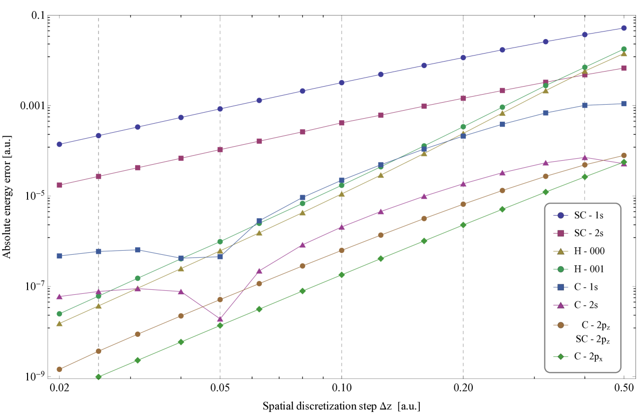
We computed the eigenenergy values using imaginary time propagation with the second order hybrid splitting scheme outlined in Section 4.3, where the parameter was chosen suitably small to minimize the spatial errors related to the operator splitting. These energy values were also verified with real time propagation, by comparing the time dependence of the phase factor of the eigenstates with the exact time dependence of : the first two significant digits of the energy error were equal. It is worth noting that, although we used our hybrid splitting for calculations, these energy errors are related only to the spatial finite differences (that is, the 2D Crank-Nicolson scheme). For these results, it was sufficient to set the “Crank-Nicolson width” just above , further increase of did not improve the results.
| Absolute energy errors of selected stationary states | |||||||
|---|---|---|---|---|---|---|---|
| 0.4 | 0.2 | 0.1 | 0.05 | 0.025 | Order | ||
| SC-1s | |||||||
| SC-2s | |||||||
| SC- | |||||||
| C-1s | |||||||
| C-2s | |||||||
| C- | |||||||
| C- | |||||||
| H-000 | |||||||
| H-001 | |||||||
From Figure 2 and Table 2 we can draw several conclusions. In the case of the 3D harmonic oscillator (a reasonably smooth potential), the method is fourth order accurate in , as expected (the effective order is higher than 4 due to the fifth order accurate second derivatives). For the Coulomb potential, things get considerably more elaborate. In the Soft-Coulomb case (SC), the energies of the states converge with second order (more precisely, with 1.86), meaning the method will not be sufficiently accurate or fast. However, for the true singular Coulomb case (C), the accuracy of the states drastically improve by two orders of magnitude around . On the other hand, the complicated step size dependence of the energy error, shown by the corresponding lines in Figure 2, does not allow for a true effective order valid in the inspected range. However, our algorithm does decrease the error with high order (close to 4) when , which is anyhow that range where the computation runtime is reasonable. The unusual step size dependence of the energy error below for data sets C-1s, C-2s is due to finite differencing with high spatial accuracy applied to a non-analytic problem ( is not continuously differentiable in the origin), along with the artificially high order boundary condition.
The test cases with work reasonably well for the configuration both with C and SC: the SC- or the C- case has better (relative) accuracy than H-000 but its order is only as shown in Figure 2. A slightly higher order of is achieved for C- (the only test case with ) which has the best accuracy of all computed eigenenergies in this Section.
In conclusion, the numerical error of the hybrid splitting algorithm displays a high order scaling with the spatial step size for the stationary states of the 3D Hydrogen problem.
6.2 Forced harmonic oscillator
In the previous section we focused on the spatial errors in conjunction with the singular Coulomb potential, now we turn our attention to the total error of the hybrid splitting algorithm using a smooth time-dependent potential. This total error is composed typically of several terms related to the finite differences, to the Padé-approximation, to the factorization of the exponential operator, and to the short time splitting of the evolution operator.
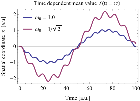
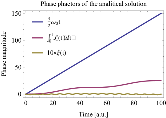
We use the so called forced harmonic oscillator (FHO) problem as the test case, defined by the potential , having a known analytical solution, which we summarize in C. Here we only illustrate this time-dependent analytical solution in Figure 3.
For error calculations, we compare the analytical and time-dependent wavefunctions at a fixed time instant by calculating the so called mean-square error, which provides information about both the total phase and the amplitude related errors. We define the mean-square error by
| (99) |
We choose the mean-square error as the reference error type because (according to our experience) it is the most reliable evolution error quantifier at a fixed time instant .
| ID | Propagation Method | Evaluations of |
|---|---|---|
| S2 | Second order operator hybrid splitting scheme (Sec. 4.3). | 1 |
| S4E3 | S2 based 4th order iterative splitting scheme using eq. (48) with . | 3 |
| S6E5 | S2 based 6th order iterative splitting scheme using eq. (49) with . | 5 |
| S6E9 | S2 based 6th order iterative splitting scheme using eq. (48) with . | 9 |
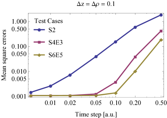
We tested our algorithm with different split-operators (listed in Table 3), and several and configurations to acquire a top-down view of the error properties of the hybrid splitting method.
The mean-square error of the different high order split-operators based on our Crank-Nicolson scheme (CN5) can be found in Table 4, and also in Figure 4: the standard convergence of the S2 scheme is very slow, and there is a drastic improvement using S4E3 on top of S2. Using either S6E9 or S6E5 does not yield much gain in accuracy compared to the their higher numerical costs. Based on these, we propose to use the fourth order split-operator method S4E3 in accordance with (48), along with our hybrid splitting scheme.
| Calculated error values at | |||||||
|---|---|---|---|---|---|---|---|
| 0.5 | 0.2 | 0.1 | 0.05 | 0.02 | 0.01 | 0.005 | |
| S2 | |||||||
| S4E3 | |||||||
| S6E5 | |||||||
| S6E9 | |||||||
| Calculated error values at | |||||||
|---|---|---|---|---|---|---|---|
| 0.5 | 0.2 | 0.1 | 0.05 | 0.02 | 0.01 | 0.005 | |
| S2 | 1.83 | ||||||
| S4E3 | |||||||
| S6E5 | |||||||
| S6E9 | |||||||
| Calculated error values at | |||||||
|---|---|---|---|---|---|---|---|
| 0.5 | 0.2 | 0.1 | 0.05 | 0.02 | 0.01 | 0.005 | |
| S2 | |||||||
| S4E3 | |||||||
| S6E5 | |||||||
| S6E9 | |||||||
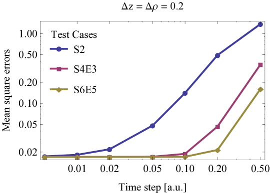
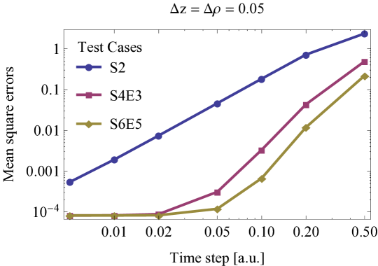
The lines corresponding to the different split-operators in Figure 4 should exhibit the expected power scaling with , this is only approximately the case and only above a threshold . Below this threshold the total error is not reduced by decreasing , because the evolution error is dominated by the finite differences: the error magnitudes can even be predicted as the product of the stationary energy error (Table 2) and the propagation time interval.
| Calculated error values of CN3 based S4E3 method | |||||||
|---|---|---|---|---|---|---|---|
| 0.5 | 0.2 | 0.1 | 0.05 | 0.02 | 0.01 | 0.005 | |
One objective of our research was to design a real space finite difference algorithm that achieves fourth order accuracy in the spatial step size and, most importantly, that is capable to include both the singular coordinate and the singular Coulomb potential directly. Therefore, it is interesting to globally benchmark the results against a second order 3-point Crank-Nicolson finite difference scheme (CN3), which means we degraded the core algorithm to use three-point finite differences in S2.
We repeated the main tests with this CN3 method combined with the split-operator configuration S4E3 (discussed above). The CN3 results are shown in Table 5 and are to be compared to the results with CN5 in Table 4. Both the CN3 and CN5 schemes display the expected order scaling of the error with . Comparing the error at (which is already below the threshold ), our fourth order discretization has one, two and three orders of magnitudes smaller errors at spatial step sizes , respectively. Thus, one should always use (at least) the CN5 scheme unless the exotic nature of the problem prevents high order discretization.
In conclusion, our hybrid splitting propagation method is suitable for numerical simulations with time-dependent Hamiltonians, and it is capable of high order scaling with , once it is incorporated into the proper high order evolution operator formulae.
6.3 Hydrogen atom in an external electric field
Finally, we conducted a test similar to real world applications by simulating the hydrogen atom in an external laser field. Now, we compare our hybrid splitting based CN5 implementation, including Coulomb potential and the Coulomb boundary condition (CN5-C) against the commonplace CN3 discretization with the best Soft-Coulomb potential approximation allowed by the spatial grid (CN3-SC), which is the same approximation that we tested in Section 6.1. We did not use the full 2D CN3 method, but we applied the hybrid splitting scheme using the CN3 equations just like the case of the FHO.
The external field was parametrized as . The simulated time was , and it consisted of only one field cycle, by setting in atomic units. The field amplitude was , with simulation box size , to contain the escaping electron waves. The initial state was the ground state, found by imaginary time propagation method to remove spurious ionization components. We use the S4E3 high order split operator formula as indicated in the last section.
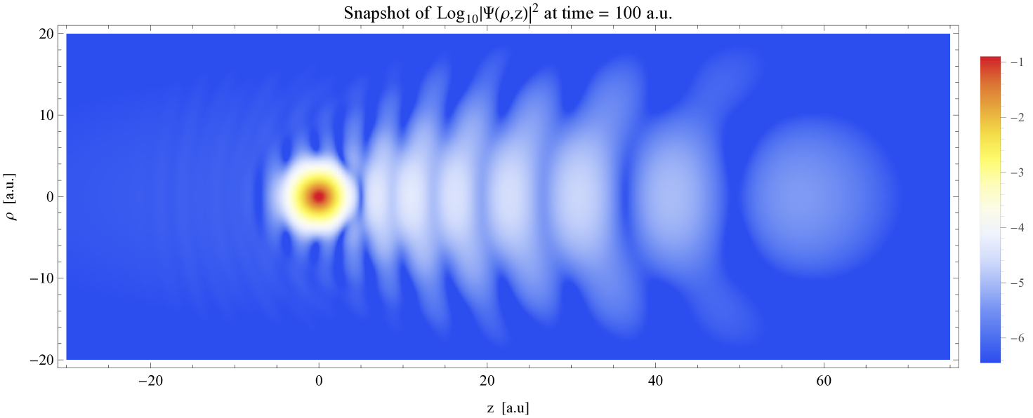
We show the result of this simulation in Figure 5 by a density plot of the logarithm of the absolute square of the wave function, in a plane containing the axis. The white waves on the right of the spherical peak, bound by the Coulomb potential of the nucleus, are ca. 4-5 order smaller in density. These waves have to be computed very accurately, since they contribute the most to the time dependence of the dipole moment, which in turn is of fundamental importance regarding the HHG and the creation of attosecond light pulses.
The tests to compare CN5-C with CN3-SC were run with and with time step if not indicated explicitly. We quantified the accuracy of the solutions with the error of the expectation value , i.e. the magnitude of the time-dependent dipole moment. Unlike the FHO example, analytic solution is not available this time, so we use a converged solution to determine numerical errors, that is we compare the results with a much more accurate numerical solution obtained using smaller , discretization steps.
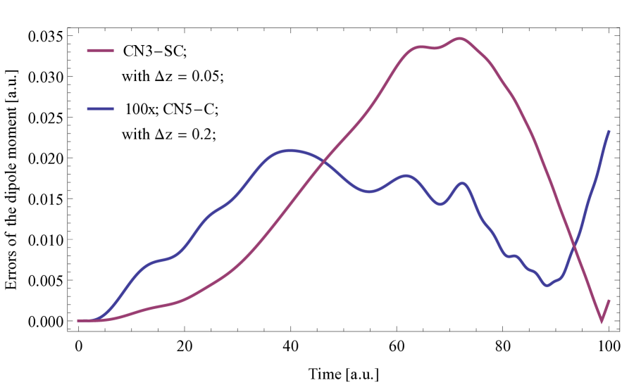
The results, shown in Figure 6 are as expected: the error of the CN5-C scheme with is smaller by two orders of magnitude than that of the CN3-SC scheme with . Based on this, we estimate the performance difference as follows. Due to the second order convergence of the CN3-SC scheme, is needed to achieve the accuracy of the CN5-C with , which means a factor of in the number of spatial gridpoints, implying a factor of - in runtime. That is, the CN5-C scheme is ca. 1000 times more effective than the CN3-SC. Regarding absolute accuracy, the magnitude of the error of using CN5-C with is smaller than the error of the FHO at the time instant , as can be seen in Table 4.
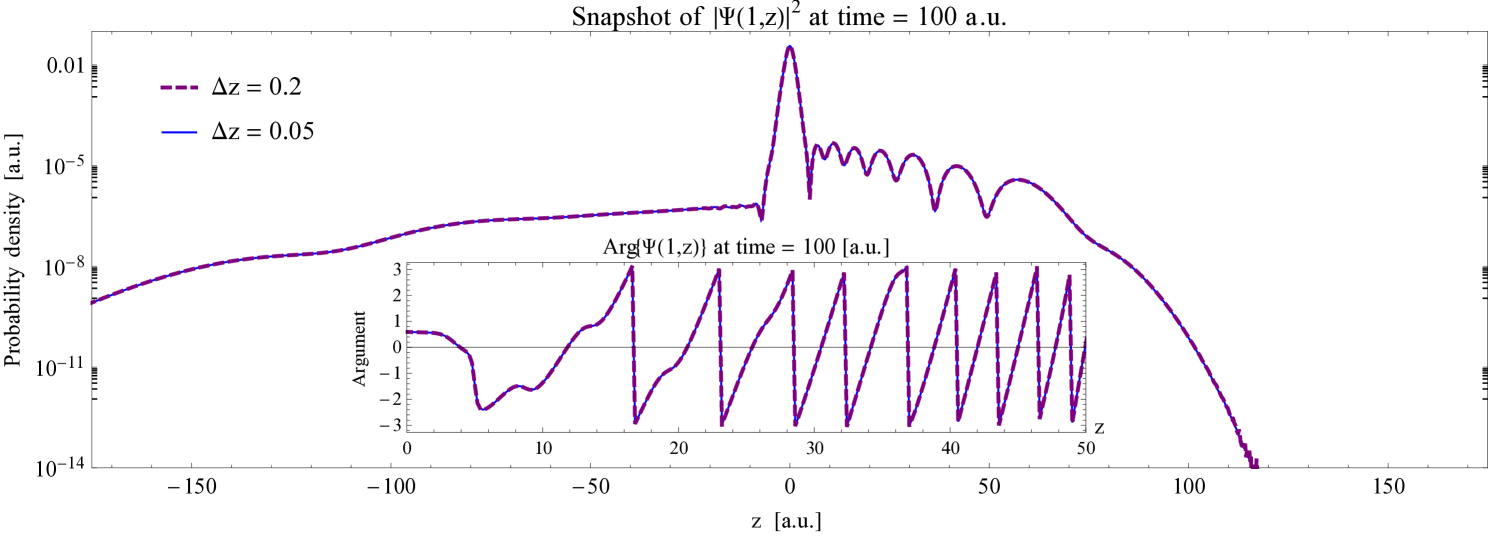
Regarding the pointwise convergence of the solution with the CN5-C method, we compare the density and the phase along a -line section at , computed with two different values of . These plots, shown in Figure 7, convincingly show that a converged numerical solution is obtained already at . Note that the accuracy of the phase is crucial in strong field physics, regarding e.g. exit momentum calculations [13, 67] in optical tunneling or regarding phase space methods [68, 69, 70, 71, 72, 73] (where usually the Wigner function is computed from the wave function and this is then further analysed for the physical interpretation of the process).
7 Summary
In this article we presented an algorithm capable of the direct numerical solution of the three dimensional time dependent Schrödinger equation, assuming axial symmetry in cylindrical coordinates. The main feature of the algorithm is that it is capable to accurately handle singular Coulomb potentials besides any smooth potential of the form . The axial symmetry enables a two dimensional grid and the availability of the Cartesian -axis makes it easy to investigate reduced electron dynamics.
We choose a high order finite difference representation in the spatial coordinate domain. We implemented all singularities that can be reduced to the form or via Neumann and Robin boundary conditions at the axis. The accuracy of the algorithm is fourth order in , for smooth potentials and it is close to fourth order for Coulomb potentials in a restricted discretization parameter range. We completed this algorithm by a high order scalar product formula designed for this finite difference representation.
We based our algorithm on the split-operator approximation of the evolution operator. Due to the non-separability of the Coulomb-problem in cylindrical coordinates, we constructed a special second order operator splitting scheme called hybrid splitting method. This splits the Hamiltonian matrix direction-wise like the traditional methods, but the innermost region near is excluded: here the full 2D Crank-Nicolson equations are used. This means that there are many decoupled 1D Schrödinger equations in the direction, and a 2D Schrödinger equation with a special block pentadiagonal pattern of the coefficient matrix, which has to be taken advantage of for maximum efficiency, like in our hybrid splitting solver algorithm. Thread based parallelization is supported throughout, and we also gave a way to evaluate the decoupled 1D Schrödinger equations with high spatial accuracy and efficiency.
We thoroughly investigated the spatial discretization related errors in an optimal discretization parameter range, determining detailed accuracy characteristics with or without Coulomb potential. We also verified the considerably increased accuracy for numerical simulations forced oscillator. Testing the performance of the 4th and the 6th order (iterative) split-operator factorizations built from second order hybrid splitting method, we observed a threshold value below which there is no accuracy gain. We concluded that high order (meaning at least 4th order) split-operator formula should be used in practice, accompanying the hybrid splitting algorithm.
In order to demonstrate the accuracy and performance of our hybrid splitting algorithm also in a simulation close to the planned applications, we computed the solution for a hydrogen atom in a strong time-dependent electric field of one sine period. The important waves in the probability density, having an amplitude of - relative to the peak value, were obtained accurately and efficiently.
The hybrid splitting scheme, with some minor modifications of the algorithm, is also capable to handle single or multiple coupled nonlinear time dependent Schrödinger equations, such as those arising e.g. in time-dependent density functional theory [74], time-dependent Hartree-Fock methods [75, 76] or several other areas of physics.
Acknowledgements
The authors thank W. Becker, M. G. Benedict, P. Földi, K. Varjú and S. Varró for stimulating discussions. This research has been granted by the Hungarian Scientific Research Fund OTKA under contract No. T81364. Partial support by the ELI-ALPS project is also acknowledged. The ELI-ALPS project (GOP-1.1.1-12/B-2012-000, GINOP-2.3.6-15-2015-00001) is supported by the European Union and co-financed by the European Regional Development Fund.
References
- [1] M. Hentschel, R. Kienberger, C. Spielmann, G. A. Reider, N. Milosevic, T. Brabec, P. Corkum, U. Heinzmann, M. Drescher, F. Krausz, Attosecond metrology, Nature 414 (6863) (2001) 509–513.
- [2] P. . M. Paul, E. Toma, P. Breger, G. Mullot, F. Augé, P. Balcou, H. Muller, P. Agostini, Observation of a train of attosecond pulses from high harmonic generation, Science 292 (5522) (2001) 1689–1692.
- [3] R. Kienberger, M. Hentschel, M. Uiberacker, C. Spielmann, M. Kitzler, A. Scrinzi, M. Wieland, T. Westerwalbesloh, U. Kleineberg, U. Heinzmann, et al., Steering attosecond electron wave packets with light, Science 297 (5584) (2002) 1144–1148.
- [4] M. Drescher, M. Hentschel, R. Kienberger, M. Uiberacker, V. Yakovlev, A. Scrinzi, T. Westerwalbesloh, U. Kleineberg, U. Heinzmann, F. Krausz, Time-resolved atomic inner-shell spectroscopy, Nature 419 (6909) (2002) 803–807.
- [5] A. Baltuška, T. Udem, M. Uiberacker, M. Hentschel, E. Goulielmakis, C. Gohle, R. Holzwarth, V. Yakovlev, A. Scrinzi, T. Hänsch, et al., Attosecond control of electronic processes by intense light fields, Nature 421 (6923) (2003) 611–615.
- [6] F. Krausz, M. Ivanov, Attosecond physics, Reviews of Modern Physics 81 (1) (2009) 163–234.
- [7] A. McPherson, G. Gibson, H. Jara, U. Johann, T. S. Luk, I. McIntyre, K. Boyer, C. K. Rhodes, Studies of multiphoton production of vacuum-ultraviolet radiation in the rare gases, Journal of the Optical Society of America B 4 (4) (1987) 595–601.
- [8] M. Ferray, A. L’Huillier, X. Li, L. Lompre, G. Mainfray, C. Manus, Multiple-harmonic conversion of 1064 nm radiation in rare gases, Journal of Physics B: Atomic, Molecular and Optical Physics 21 (3) (1988) L31.
- [9] G. Farkas, C. Tóth, Proposal for attosecond light pulse generation using laser induced multiple-harmonic conversion processes in rare gases, Physics Letters A 168 (5) (1992) 447–450.
- [10] S. Harris, J. Macklin, T. Hänsch, Atomic scale temporal structure inherent to high-order harmonic generation, Optics communications 100 (5-6) (1993) 487–490.
- [11] M. Uiberacker, T. Uphues, M. Schultze, A. J. Verhoef, V. Yakovlev, M. F. Kling, J. Rauschenberger, N. M. Kabachnik, H. Schröder, M. Lezius, et al., Attosecond real-time observation of electron tunnelling in atoms, Nature 446 (7136) (2007) 627–632.
- [12] S. Haessler, J. Caillat, W. Boutu, C. Giovanetti-Teixeira, T. Ruchon, T. Auguste, Z. Diveki, P. Breger, A. Maquet, B. Carré, et al., Attosecond imaging of molecular electronic wavepackets, Nature Physics 6 (3) (2010) 200–206.
- [13] A. N. Pfeiffer, C. Cirelli, A. S. Landsman, M. Smolarski, D. Dimitrovski, L. B. Madsen, U. Keller, Probing the longitudinal momentum spread of the electron wave packet at the tunnel exit, Physical Review Letters 109 (8) (2012) 083002.
- [14] D. Shafir, H. Soifer, B. D. Bruner, M. Dagan, Y. Mairesse, S. Patchkovskii, M. Y. Ivanov, O. Smirnova, N. Dudovich, Resolving the time when an electron exits a tunnelling barrier, Nature 485 (7398) (2012) 343–346.
- [15] M. Schultze, M. Fieß, N. Karpowicz, J. Gagnon, M. Korbman, M. Hofstetter, S. Neppl, A. L. Cavalieri, Y. Komninos, T. Mercouris, et al., Delay in photoemission, Science 328 (5986) (2010) 1658–1662.
- [16] A. L. Cavalieri, N. Müller, T. Uphues, V. S. Yakovlev, A. Baltuška, B. Horvath, B. Schmidt, L. Blümel, R. Holzwarth, S. Hendel, et al., Attosecond spectroscopy in condensed matter, Nature 449 (7165) (2007) 1029–1032.
- [17] A. D. Bandrauk, M. Ivanov, Quantum Dynamic Imaging: Theoretical and Numerical Methods, Springer Science & Business Media, 2011.
- [18] L. Keldysh, Ionization in the field of a strong electromagnetic wave, Soviet Physics JETP 20 (5) (1965) 1307–1314.
- [19] P. B. Corkum, Plasma perspective on strong field multiphoton ionization, Physical Review Letters 71 (13) (1993) 1994.
- [20] P. Eckle, A. Pfeiffer, C. Cirelli, A. Staudte, R. Dörner, H. Muller, M. Büttiker, U. Keller, Attosecond ionization and tunneling delay time measurements in helium, Science 322 (5907) (2008) 1525–1529.
- [21] M. Lewenstein, P. Balcou, M. Y. Ivanov, A. L’Huillier, Auillier, P. B. Corkum, Theory of high-harmonic generation by low-frequency laser fields, Physical Review A 49 (3) (1994) 2117.
- [22] M. Y. Ivanov, M. Spanner, O. Smirnova, Anatomy of strong field ionization, Journal of Modern Optics 52 (2-3) (2005) 165–184.
- [23] A. Gordon, R. Santra, F. X. Kärtner, Role of the coulomb singularity in high-order harmonic generation, Physical Review A 72 (6) (2005) 063411.
- [24] X.-M. Tong, S.-I. Chu, Theoretical study of multiple high-order harmonic generation by intense ultrashort pulsed laser fields: A new generalized pseudospectral time-dependent method, Chemical Physics 217 (2) (1997) 119–130.
- [25] H. Bachau, E. Cormier, P. Decleva, J. Hansen, F. Martin, Applications of b-splines in atomic and molecular physics, Reports on Progress in Physics 64 (12) (2001) 1815.
- [26] E. Cormier, P. Lambropoulos, Above-threshold ionization spectrum of hydrogen using b-spline functions, Journal of Physics B: Atomic, Molecular and Optical Physics 30 (1) (1997) 77.
- [27] H. Muller, An efficient propagation scheme for the time-dependent Schrödinger equation in the velocity gauge, Laser Physics 9 (1999) 138–148.
- [28] D. Bauer, P. Koval, Qprop: A Schrödinger-solver for intense laser–atom interaction, Computer Physics Communications 174 (5) (2006) 396–421.
- [29] E. S. Smyth, J. S. Parker, K. T. Taylor, Numerical integration of the time-dependent Schrödinger equation for laser-driven helium, Computer Physics Communications 114 (1) (1998) 1–14.
- [30] L. Argenti, R. Pazourek, J. Feist, S. Nagele, M. Liertzer, E. Persson, J. Burgdörfer, E. Lindroth, Photoionization of helium by attosecond pulses: Extraction of spectra from correlated wave functions, Physical Review A 87 (5) (2013) 053405.
- [31] B. I. Schneider, L. A. Collins, S. Hu, Parallel solver for the time-dependent linear and nonlinear Schrödinger equation, Physical Review E 73 (3) (2006) 036708.
- [32] A. Kołakowska, M. Pindzola, F. Robicheaux, D. Schultz, J. Wells, Excitation and charge transfer in proton-hydrogen collisions, Physical Review A 58 (4) (1998) 2872.
- [33] I. P. Christov, M. M. Murnane, H. C. Kapteyn, High-harmonic generation of attosecond pulses in the single-cycle regime, Physical Review Letters 78 (7) (1997) 1251.
- [34] S. Hu, L. Collins, Intense laser-induced recombination: The inverse above-threshold ionization process, Physical Review A 70 (1) (2004) 013407.
- [35] J. Wells, D. Schultz, P. Gavras, M. Pindzola, Numerical solution of the time-dependent Schrödinger equation for intermediate-energy collisions of antiprotons with hydrogen, Physical Review A 54 (1) (1996) 593.
- [36] A. Gordon, C. Jirauschek, F. X. Kärtner, Numerical solver of the time-dependent Schrödinger equation with coulomb singularities, Physical Review A 73 (4) (2006) 042505.
- [37] I. Gainullin, M. Sonkin, High-performance parallel solver for 3d time-dependent Schrödinger equation for large-scale nanosystems, Computer Physics Communications 188 (2015) 68–75.
- [38] C. Leforestier, R. Bisseling, C. Cerjan, M. Feit, R. Friesner, A. Guldberg, A. Hammerich, G. Jolicard, W. Karrlein, H.-D. Meyer, et al., A comparison of different propagation schemes for the time dependent Schrödinger equation, Journal of Computational Physics 94 (1) (1991) 59–80.
- [39] T. Iitaka, Solving the time-dependent Schrödinger equation numerically, Physical Review E 49 (5) (1994) 4684.
- [40] A. Castro, M. A. Marques, A. Rubio, Propagators for the time-dependent Kohn–Sham equations, The Journal of chemical physics 121 (8) (2004) 3425–3433.
- [41] S. Blanes, P. Moan, Splitting methods for the time-dependent Schrödinger equation, Physics Letters A 265 (1) (2000) 35–42.
- [42] S. A. Chin, C.-R. Chen, Fourth order gradient symplectic integrator methods for solving the time-dependent Schrödinger equation, The Journal of Chemical Physics 114 (17) (2001) 7338–7341.
- [43] W. H. Press, S. A. Teukolsky, W. T. Vetterling, B. P. Flannery, Numerical Recipes 3rd Edition: The Art of Scientific Computing, 3rd Edition, Cambridge University Press, 2007.
- [44] I. Puzynin, A. Selin, S. Vinitsky, A high-order accuracy method for numerical solving of the time-dependent Schrödinger equation, Computer Physics Communications 123 (1) (1999) 1–6.
- [45] H. Wang, Numerical studies on the split-step finite difference method for nonlinear Schrödinger equations, Applied Mathematics and Computation 170 (1) (2005) 17–35.
- [46] J. Shen, E. Wei, Z. Huang, M. Chen, X. Wu, High-order symplectic fdtd scheme for solving a time-dependent Schrödinger equation, Computer Physics Communications 184 (3) (2013) 480–492.
- [47] B. H. Bransden, C. J. Joachain, Physics of Atoms and Molecules, Pearson Education India, 2003.
- [48] C. Cohen-Tannoudji, B. Diu, F. Laloë, Quantum Mechanics, Quantum Mechanics, Wiley, 1977.
- [49] D. J. Griffiths, Introduction to Quantum Mechanics, Pearson Education India, 2005.
- [50] I. Puzynin, A. Selin, S. Vinitsky, Magnus-factorized method for numerical solving the time-dependent Schrödinger equation, Computer Physics Communications 126 (1) (2000) 158–161.
- [51] S. Blanes, F. Casas, J. Oteo, J. Ros, The magnus expansion and some of its applications, Physics Reports 470 (5) (2009) 151–238.
- [52] W. van Dijk, F. Toyama, Accurate numerical solutions of the time-dependent Schrödinger equation, Physical Review E 75 (3) (2007) 36707.
- [53] J. M. Varah, On the solution of block-tridiagonal systems arising from certain finite-difference equations, Mathematics of Computation 26 (120) (1972) 859–868.
- [54] R. Wilcox, Exponential operators and parameter differentiation in quantum physics, Journal of Mathematical Physics 8 (4) (1967) 962–982.
- [55] R. I. McLachlan, G. R. W. Quispel, Splitting methods, Acta Numerica 11 (2002) 341–434.
- [56] Y. Yazici, Operator splitting methods for differential equations, Ph.D. thesis, Izmir Institute of Technology (2010).
- [57] G. Strang, On the construction and comparison of difference schemes, SIAM Journal on Numerical Analysis 5 (3) (1968) 506–517.
- [58] S. A. Chin, Symplectic integrators from composite operator factorizations, Physics Letters A 226 (6) (1997) 344–348.
- [59] M. Suzuki, Hybrid exponential product formulas for unbounded operators with possible applications to monte carlo simulations, Physics Letters A 201 (5) (1995) 425–428.
- [60] A. D. Bandrauk, H. Shen, Higher order exponential split operator method for solving time-dependent Schrödinger equations, Canadian Journal of Chemistry 70 (2) (1992) 555–559.
- [61] A. D. Bandrauk, H. Lu, Exponential propagators (integrators) for the time-dependent Schrödinger equation, Journal of Theoretical and Computational Chemistry 12 (06) (2013) 1340001.
- [62] A. D. Bandrauk, H. Shen, Exponential split operator methods for solving coupled time-dependent Schrödinger equations, The Journal of chemical physics 99 (2) (1993) 1185–1193.
- [63] S. A. Chin, S. Janecek, E. Krotscheck, Any order imaginary time propagation method for solving the Schrödinger equation, Chemical Physics Letters 470 (4) (2009) 342–346.
- [64] L. Lehtovaara, J. Toivanen, J. Eloranta, Solution of time-independent Schrödinger equation by the imaginary time propagation method, Journal of Computational Physics 221 (1) (2007) 148–157.
- [65] J. G. Muga, J. Palao, B. Navarro, I. Egusquiza, Complex absorbing potentials, Physics Reports 395 (6) (2004) 357–426.
- [66] A. Karawia, A computational algorithm for solving periodic penta-diagonal linear systems, Applied Mathematics and Computation 174 (1) (2006) 613–618.
- [67] X. Sun, M. Li, J. Yu, Y. Deng, Q. Gong, Y. Liu, Calibration of the initial longitudinal momentum spread of tunneling ionization, Physical Review A 89 (4) (2014) 045402.
- [68] A. Czirják, R. Kopold, W. Becker, M. Kleber, W. Schleich, The Wigner function for tunneling in a uniform static electric field, Optics communications 179 (1) (2000) 29–38.
- [69] L. Guo, S. Han, J. Chen, Time-energy analysis of above-threshold ionization in few-cycle laser pulses, Physical Review A 86 (5) (2012) 053409.
- [70] S. Gräfe, J. Doose, J. Burgdörfer, Quantum phase-space analysis of electronic rescattering dynamics in intense few-cycle laser fields, Journal of Physics B: Atomic, Molecular and Optical Physics 45 (5) (2012) 055002.
- [71] A. Czirják, S. Majorosi, J. Kovács, M. G. Benedict, Emergence of oscillations in quantum entanglement during rescattering, Physica Scripta 2013 (T153) (2013) 014013.
- [72] C. Zagoya, J. Wu, M. Ronto, D. Shalashilin, C. F. de Morisson Faria, Quantum and semiclassical phase-space dynamics of a wave packet in strong fields using initial-value representations, New Journal of Physics 16 (10) (2014) 103040.
- [73] C. Baumann, H.-J. Kull, G. Fraiman, Wigner representation of ionization and scattering in strong laser fields, Physical Review A 92 (6) (2015) 063420.
- [74] C. A. Ullrich, Z.-h. Yang, A brief compendium of time-dependent density functional theory, Brazilian Journal of Physics 44 (1) (2014) 154–188.
- [75] K. C. Kulander, Time-dependent Hartree-Fock theory of multiphoton ionization: Helium, Physical Review A 36 (6) (1987) 2726.
- [76] M. Pindzola, D. Griffin, C. Bottcher, Validity of time-dependent Hartree-Fock theory for the multiphoton ionization of atoms, Physical Review Letters 66 (18) (1991) 2305.
- [77] C. A. Moyer, Numerov extension of transparent boundary conditions for the Schrödinger equation in one dimension, American Journal of Physics 72 (3) (2004) 351–358.
- [78] K. Husimi, Miscellanea in elementary quantum mechanics, ii, Progress of Theoretical Physics 9 (4) (1953) 381–402.
Appendix A Approximating the inner product
In this Section we propose a solution to the problem of the discrete inner product formula exposed in Section 3.2.
We seek a discretized representation of the inner product formula in the cylindrical coordinate system as
| (100) |
The naive approach with coefficients causes inaccuracy which originates from the edge and its neighborhood only, because the formula with this particular has exponential convergence at the box boundaries [43].
Besides the accuracy, the conservation of a discretized scheme of form (100) is also an issue: given a discrete Hamiltonian matrix in the Padé-approximation then the time evolution will be unitary with respect to the inner product only if is self-adjoint. Unfortunately, because of the Neumann and Robin boundary conditions (38) the Hamiltonian matrix does not exist on the line, therefore there is no standard norm of form which is perfectly conserved by the numerical scheme.
Therefore, our aim is to approximate (100) with an order that is higher than the order of the finite difference scheme. To achieve this goal, we used Lagrange [43] interpolating polynomial defined on points , , , , , , for a given line, where is the integrand in . We use an elementary integral formula between and :
| (101) |
We sum up this for all points, and utilize the boundary conditions for , then we arrive at the following integral formula, which is our choice to approximate the scalar product (100):
| (102) |
This achieves the high integration accuracy (it is exact for a polynomial of up to degree 6), which is needed: the computed norm variations become proportional to , which is consistent with the accuracy of the spatial finite differences. The constructed Crank-Nicolson scheme stayed stable in our simulations.
Appendix B Numerov z-line propagator algorithm
We have constructed an efficient way of evaluating line-by-line, based on the second order Crank-Nicolson algorithm with Numerov-extension [77], which also provides at least fourth order accuracy in , and it reduces the numerical costs because it uses three point finite differences and tridiagonal equations instead of five point differences and pentadiagonal equations. We will also outline an optimization technique for 1D Crank-Nicolson schemes which is makes the computations even more efficient when they are applied to 2D problems.
Let us fix the value of coordinate (i.e we choose ) and we denote . Here we consider the Hamiltonian in the form of along this line, since the procedure below allows to include a potential of this form, which is however not present in our hybrid splitting scheme. Again, we start with the second order approximation of the exponential operator as in (27)
| (103) |
with , . We will use a discretized Laplacian based on the standard three point finite difference method [43], however, we will also need the leading term of the error:
| (104) |
To proceed, we introduce the auxiliary variable and rewrite the equation (103) as
| (105) |
Then, we discretize the equation (105) using (104):
| (106) |
Now, we evaluate the error term with also using the right hand side of (105) to get to the result of the form
| (107) |
Restoring the equations for we arrive at the Numerov-extended Crank-Nicolson algorithm as
| (108) |
It is interesting to note that by reverse engineering from the Padé-form, we get a discrete Hamiltonian of the form
| (109) |
The extra terms in (109) improve the solution to fifth order in , however, one should note that (i) is part of , requiring the potential to be continuously differentiable, (ii) is no longer strictly self-adjoint.
In (108) we have arrived at a tridiagonal system of linear equations of the form
| (110) |
which after forward Gaussian-elimination reads
| (111) |
| (112) |
| (113) |
| (114) |
| (115) |
The right hand side and the solution of (111) are given by the following expressions:
| (116) |
| (117) |
This completes the 1D propagation method.
Now let us return to our original 2D problem. Because the discrete Hamiltonian is independent from the value of , the corresponding coefficient matrix of (111) is the same for each -line. This means that we need to do the forward elimination (115) only once, then it is sufficient to perform only the forward (116) and the backward substitution (117) steps for each -line in order to acquire the solution. This yields a factor of 2 speedup in the evaluation of with three point finite differences, if we have many lines to propagate and cache the appropriate variables. This latter can also be viewed as an LU decomposition based optimization [43].
Appendix C Analytical solution of the forced harmonic oscillator
The TDSE for the axially symmetric (i.e. ) 3D forced harmonic oscillator (FHO) in cylindrical coordinates is the following:
| (118) |
where . Using the separability in and coordinates, we can reduce this problem to a one dimensional time-dependent one, which was solved by K. Husimi et. al. [78]. Then, the analytical time-dependent wave function is of the form
| (119) |
where is a solution of the 3D field-free quantum harmonic oscillator problem with axial symmetry. We define it to be the ground state of the field-free problem (H-000):
| (120) |
In formula (119) the symbol denotes the Lagrangian of the corresponding classical system:
| (121) |
and is the solution of the initial value problem
| (122) |
We set , then the previous equation is that of the forced harmonic oscillator has the solution:
| (123) |