FOXTAIL: Modeling the nonlinear interaction between
Alfvén eigenmodes and energetic particles in tokamaks
Abstract
FOXTAIL is a new hybrid magnetohydrodynamic–kinetic code used to describe interactions between energetic particles and Alfvén eigenmodes in tokamaks with realistic geometries. The code simulates the nonlinear dynamics of the amplitudes of individual eigenmodes and of a set of discrete markers in five-dimensional phase space representing the energetic particle distribution. Action–angle coordinates of the equilibrium system are used for efficient tracing of energetic particles, and the particle acceleration by the wave fields of the eigenmodes is Fourier decomposed in the same angles. The eigenmodes are described using temporally constant eigenfunctions with dynamic complex amplitudes. Possible applications of the code are presented, e.g., making a quantitative validity evaluation of the one-dimensional bump-on-tail approximation of the system. Expected effects of the fulfillment of the Chirikov criterion in two-mode scenarios have also been verified.
keywords:
Magnetohydrodynamic waves , Tokamaks , Fast particle effects , Nonlinear dynamics , Hybrid plasma simulation methods , Lagrangian and Hamiltonian mechanicsPACS:
05.45.-a , 45.20.Jj , 52.35.Bj , 52.55.Fa , 52.55.Pi , 52.65.Ww1 Introduction
Toroidal Alfvén eigenmodes (TAEs) are discrete frequency MHD waves that exist in the toroidicity induced gap of the Alfvén continuum spectra in toroidal magnetized plasmas. TAEs are typically excited by an ensemble of energetic ions (e.g. coming from auxiliary heating or from fusion reactions) with an inverted energy distribution along the characteristic curves of wave–particle interaction in momentum space. If these waves are excited to large amplitudes, they might eject a large fraction of energetic ions from the plasma before the ions transfer their energy to the bulk plasma, causing a significant reduction of heating efficiency of fast ions [1, 2]. It is therefore of great importance to understand the significance of TAEs in future devices, such as ITER. Accurate modeling is required that can resolve the nonlinear evolution of the wave–particle interactions.
Many hybrid MHD–kinetic Monte Carlo codes developed for this purpose are orbit following, requiring temporal resolutions well below bounce time scales of the resonant energetic particles. These are many orders of magnitude shorter than the time scales for the relevant dynamics of long-lived eigenmodes in large tokamaks, such as ITER. Relatively simple equations of motion that can resolve the relevant time scales for wave–particle interaction more efficiently can be acquired by using action–angle coordinates [3] of the equilibrium system for the phase space of energetic particles. Particles in the unperturbed equilibrium system then follow straight lines in configuration space at constant velocities, and their canonical momenta are constants of motion. This coordinate system has the advantage that particles exactly remain on their guiding center orbits in the unperturbed system, independently of the time step length.
In order to get satisfactory convergence of the Monte Carlo codes describing nonlinear wave–particle interactions, methods are often used. Although the method is computationally advantageous, it makes the code more difficult to use in conjunction with existing Monte Carlo codes that use full- methods or that use a different background distribution.
FOXTAIL (“FOurier series eXpansion of fasT particle–Alfvén eigenmode Interaction”-modeL) is a new hybrid magnetohydrodynamic–kinetic model that both uses action–angle coordinates for particle phase space and a full- Monte Carlo method to represent the resonant energetic particle distribution. It is based on a model by Berk et al. [4], which is derived from a Lagrangian formulation of the wave–particle interaction. The use of action–angle variables can give scenarios where the shortest time scale needed to be resolved in FOXTAIL is on the order of , where is the precession frequency of the energetic particles interacting strongly with the eigenmodes.
A simplification used in FOXTAIL is that the spatial structures of the eigenmode wave fields are taken to be constant in time. This limitation means that FOXTAIL is unable to model, e.g., energetic particle modes. There also exist scenarios where the time evolution of TAE eigenfunctions is of importance (see e.g. Ref. [5]). Such scenarios can be modeled by other existing codes, not having the limitation of static eigenfunctions, such as the hybrid MHD–gyrokinetic code, HMGC [6, 7, 8], and the gyrokinetic toroidal code, GTC [9, 10, 11].
The structure of this paper is the following: Section 2 presents the mathematical, the physical and the technical background of FOXTAIL, including derivations of the equations used in the different parts of the code and the overall structure of the code. Section 3 describes how some of the resulting equations are numerically implemented. Section 4 presents some of the possible applications of FOXTAIL, including quantitative comparisons with the corresponding one-dimensional bump-on-tail approximation of the system and numerical studies of the Chirikov criterion in scenarios with two eigenmodes. Section 5 summarizes the paper.
2 Model description
2.1 Physics overview
The equations used in FOXTAIL are based on a Lagrangian formulation of the wave–particle system [4]. Each simulation is formulated as an initial value problem, starting from an energetic particle distribution in a background equilibrium plasma and a set of eigenmodes with a static spatial structure and a dynamical amplitude and phase. Eigenmodes are treated as weak perturbations of the equilibrium, excluding direct mode–mode interaction. The nonlinear coupling of eigenmodes is taken into account only by the energy and momentum exchange between the modes via the energetic particles.
The physical process of the considered wave–particle interactions is essentially absorption and stimulated emission, and the interactions are energy and momentum conserving. The total energy of the eigenmode is proportional to the amplitude squared. Energy conservation is ensured by the equation
| (1) |
where is the time derivative of the kinetic particle energy, as accelerated by the wave field, is the complex amplitude of the eigenmode, and is the ratio between the eigenmode energy and . A Lagrangian formulation of the wave–particle interaction is presented in section 2.7, which is shown to be consistent with eq. (1).
The acceleration of a particle by an Alfvén eigenmode convects the momentum of the particles along curves in the phase space according to
| (2) |
where is the particle kinetic energy, is the toroidal canonical momentum, is the magnetic moment, is the toroidal mode number of the eigenmode and is the eigenmode frequency. The magnetic moment is unperturbed, since the Alfvén eigenmodes are low frequency waves (). The curves in -space specified by eq. (2) are referred to as the characteristic curves of wave–particle interaction. Within certain parameter limits, FOXTAIL is equivalent with a one-dimensional bump-on-tail model describing the wave–particle interaction (cf. Ref. [12]). Different characteristic curves are indistinguishable in this limit, and the momentum of the 1D model then corresponds to a variable indexing the location of the particle along the characteristic curves. From the theory of the 1D bump-on-tail model, it is apparent that an inverted energy distribution along the characteristic curves at the wave–particle resonance can excite eigenmodes via a process analogous to Landau damping.
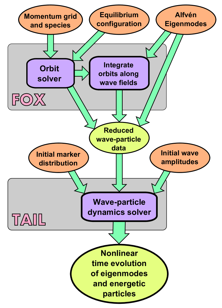
2.2 Overview of the FOXTAIL code
The FOXTAIL code is essentially split into two parts, “FOX” and “TAIL”, as illustrated in Fig. 1. TAIL is the numerical dynamics solver of the eigenmodes and the energetic particles, solving the wave–particle system as an initial value problem. FOX can be viewed as a preprocessor of TAIL, calculating orbital, eigenmode and interaction related data for a given set of eigenmodes and energetic particle species in a defined equilibrium configuration. The distribution of energetic particles is represented using a finite set of markers with predefined weights.
2.3 Action–angle coordinates
The phase space of markers in TAIL is described using action–angle coordinates of the equilibrium system [3]. The equations of motion of the system become particularly simple in this choice of coordinates, which contributes to the computational efficiency of the solver. In the absence of wave field perturbations, the “action” coordinates (i.e. the momentum coordinates of the canonical action–angle coordinate system) are constants of motion, whereas the “angle” coordinates (configuration space coordinates) evolve with constant velocities. The presence of eigenmodes perturbs this simple dynamics, and the adiabatic invariants are convected according to eq. (2).
The angle coordinates of the system are given by
| (3) |
where is the gyro-angle, and are the poloidal and toroidal angles, respectively, are the action coordinates, canonical to the angles . Furthermore, () is the (time averaged) gyro-frequency and and are the bounce and precession frequencies, respectively. The integrals of eq. (3) are evaluated on the poloidal coordinates along the guiding center orbits.
FOXTAIL uses the adiabatic invariants as momentum coordinates ( is the normalized magnetic moment, where is the on-axis magnetic field strength). These momentum coordinates can be expressed as functions of . The angle coordinates are referred to as the transformed gyro-angle, poloidal angle and toroidal angle, respectively. In the equilibrium system, where the momentum coordinates are constant, the transformed angles evolve at a constant velocity . The dynamics in the FOXTAIL model is averaged over gyration time scales, and consequently is an ignorable coordinate of the system.
The transformed poloidal angle, , can be viewed as an index of the location of the particle in the guiding center orbit, where is a complete period of the guiding center orbit in the poloidal plane ( is defined as the point where the outer leg of the orbit intersects with the equatorial plane). In section 2.5, it is shown that a Fourier expansion of the instant acceleration of the particle in the wave field is a convenient representation of the wave–particle interactions.
Complications arise for the coordinate close to the boundary , where the particle asymptotically approaches one of the turning points. In this limit, all points along the orbit besides the turning points are represented by infinitely narrow intervals in , and the representation of the wave–particle interaction using Fourier series expansions in -space becomes invalid. These complications can potentially be resolved either by ad hoc boundary conditions or by more sophisticated coordinate transformations close to this boundary. However, all of the numerical studies presented in this paper consider scenarios where the simulated energetic particle distributions are sufficiently far from the boundary.
2.4 Orbit solver
FOX contains subroutines that solves the 3D motion of particles in a given equilibrium field configuration on a grid in -space. The equilibrium configuration and the particle orbits are described in -space, where is the poloidal magnetic flux per radian. For each orbit on the -grid, the time evolution of , and is calculated, where is the shifted toroidal coordinate ( is shifted such that coincides with ). The equilibrium configuration is taken to be axisymmetric. Assuming MHD force balance and nested magnetic flux surfaces, the equilibrium magnetic field can be expressed as
| (4) |
The guiding center motion consists of a parallel motion and a drift motion, where the drift is given by the combined , and curvature drifts according to
| (5) |
By combining with and eliminating , it can be shown that the coordinates of the guiding center orbits in the poloidal plane follow the equation
| (6) |
where
| (7) |
| (8) |
is the covariant toroidal component of the drift velocity, and are the contravariant -components of and , respectively, and is the particle mass.
Once the projections of the orbits on the poloidal plane are solved on the chosen -grid using eq. (6), the corresponding time coordinates are calculated according to
| (9) |
where
| (10) |
| (11) |
and is defined as the point where the outer leg of the guiding center orbit intersects the equatorial plane (). Similarly, the coordinates are calculated from the toroidal velocity according to
| (12) |
where
| (13) |
When calculating the wave–particle interaction coefficients, the poloidal velocity is required at each point of the orbit (see eq. (22)). It is given by
| (14) |
2.5 Wave field description
The present version of FOXTAIL describes the dynamics of low frequency, shear eigenmodes, such as the toroidal Alfvén eigenmodes (TAEs), but the model can be extended to describe eigenmodes with, e.g., compressible components as well.
Neglecting plasma resistivity, the general electric wave field can be represented by the two scalar potentials and according to
| (15) |
where the first term is associated with magnetic shear, and the second term is associated with magnetic compression. When parallel gradients in the plasma are negligible in comparison to perpendicular gradients, the excitation of the two scalar potentials and is almost decoupled, and it is sufficient to describe the shear Alfvén wave using the first term [4].
In an axisymmetric toroidal plasma, the scalar potential of each eigenmode (indexed by ) can be written on the form
| (16) |
where and are the slowly varying amplitude and phase of the eigenmode, respectively (, ), is the toroidal mode number and is the eigenmode frequency. The electric wave field therefore given by
| (17) |
where
| (18) |
.
2.6 Fourier series expansion of fast particle–Alfvén eigenmode interaction
The acceleration of the energetic particle in the wave field is described by the equation
| (19) |
where averages over the gyro-motion. Initial versions of FOXTAIL only consider the lowest order averaging over the gyro-motion, but gyro-kinetic corrections to the averaging may be included in later versions. The averaged can be written as
| (20) |
where averages the parallel magnetic wave field over the surface enclosed by the gyro-ring (generated by the span of the gyro-angle. For shear waves, the term can be neglected, and we are left with
| (21) |
where
| (22) |
, and are the guiding center velocities, given by eqs. (10), (2.4) and (13), respectively, and , and are given by eq. (18).
All guiding center coordinates and their velocities can be written as functions of and . It is then possible to write on a very compact form using action–angle coordinates:
| (23) |
where
| (24) |
The coefficients are the Fourier series expansion of the wave–particle interaction that named the FOX code. It can be seen in eq. (23) that a wave–particle resonance is characterized by the condition . The model is very efficient in the sense that one can select the relevant modes and coefficients that are close to resonant with an ensemble of energetic particles and neglect all other modes and non-resonant Fourier coefficients. If the relevant coefficients only have , becomes an ignorable coordinate of the system, and the shortest time scales that need to be resolved in simulations using TAIL are the precession time scales, .
As was mentioned in section 2.3, complications arise for the choice of action–angle coordinates when describing the wave–particle interaction in regions where . This is explicitly seen in eq. (24), where , and the integrand oscillates infinitely fast in . is bounded, and constant for all in this limit except for the infinitely narrow intervals that do not represent the turning points. For this reason, it can be understood that tends to zero towards the boundary surface. Note that the sum of eq. (23) over all integers should remain finite, given that particles can be accelerated across these surfaces by wave fields.
2.7 Lagrangian formulation of wave–particle interaction
A model for describing the dynamics of the momentum variables and the amplitudes and phases of the eigenmodes remains to be found. Such a model can be derived from a Lagrangian formulation of the wave–particle system. We consider additions to the equilibrium Lagrangian by power series of the eigenmode amplitude .
Expressed in action–angle variables, the zeroth order Lagrangian reads [13]
| (25) |
where is the particle index, and , satisfying
| (26) |
is the equilibrium Hamiltonian. A first order Lagrangian consistent with eq. (23) is
| (27) |
In a low- plasma, the second order Lagrangian for shear Alfvén eigenmodes can be expressed on the form [4]
| (28) |
when neglecting rapidly oscillating terms (on time scales ), where is the vacuum permeability.
Note that the system is invariant under the transformation , for any constant . A normalization can be imposed by the condition
| (29) |
for each mode . Then the second order Lagrangian reduces to
| (30) |
Assuming that the amplitudes are small enough, such that , the corresponding Hamiltonian for the wave–particle system is , with the canonically conjugate pairs , , and . From this, one can derive all the remaining equations of motion of the wave–particle system self-consistently.
Defining the complex amplitude and using that , the equations of motion of the wave–particle system is
| (31) |
where
| (32) |
2.8 Additional operators
The effects of particle collisions are not covered by the theory presented in the preceding sections. These effects can be added explicitly to the system, e.g. by using a diffusion operator in momentum space [14] combined with a momentum drag [15] derived from the Fokker–Planck operator, which act directly on the energetic particle distribution. Adding diffusion to the system transforms the system of ordinary differential equations in eq. (31) to a system of stochastic differential equations. The general drag–diffusion operator can be written on Itō form according to
| (33) |
where is associated with drag, is associated with diffusion and the components of are independent Wiener processes in time. Both and are functions of and in general, but orbit averaged (i.e. averaged) versions of the operators may be used for simplicity (see e.g. Ref. [16]).
There are other processes external to the energetic particle–Alfvén eigenmode system which may be included. Depending on the source of the energetic particle distribution (e.g. neutral beam injection, cyclotron resonance heating or nuclear fusion), operators can be added that continuously supply particles and/or energy to the system. Particle sources are typically modeled by dynamical weights and statistical redistribution of markers. Losses from Bremsstrahlung and cyclotron radiation can be modeled by additions to the terms in eq. (33).
An additional term can be added to the amplitude equation ( in eq. (31)) in order to model various damping mechanisms on the eigenmode amplitudes, where is the damping rate of the :th mode. This damping can, e.g., come from Landau damping in the interaction with thermal particles or damping due to mode conversion. The term of the amplitude equation is here referred to as explicit wave damping, unlike the Landau damping coming from the interaction with the energetic particle distribution, which arises implicitly from the model equations.
2.9 Lowest order corrections to the angle perturbation
When going from the Lagrangians of eqs. (25), (27) and (30) to eq. (31), it was assumed that , which allowed one to neglect corrections of the canonical momenta coming from the implicit dependence of with respect to and . For a small enough , the final equations for and are given only by the derivatives of the equilibrium Hamiltonian with respect to and , respectively. However, the above assumptions might not be valid for large amplitude eigenmodes and for processes affecting the energetic particles or the eigenmodes that are not direct wave–particle interaction, and one may have to consider the lowest order correction to and due to momentum perturbation. The correction can be understood from the fact that maps differently to locations on the guiding center orbit for different . Without the correction, one pushes the particle forwards or backwards along the orbit due to different mapping of .
Assuming a minimal perturbation of the guiding center position in -space while perturbing by the amount , it can be shown that should be corrected by the amount , where
| (34) |
is the distance from the symmetry axis and is the vertical guiding center position. Using that , it can be shown that
| (35) |
All the derivatives with respect to on the right hand sides of eqs. (34) and (2.9) are evaluated while keeping constant.
When the perturbations of any process is stochastic ( of eq. (33) is nonzero), the angle coordinates become stochastic as well when including the and corrections. This is typically how phase decorrelation is introduced to the system. Such an operator was analyzed for the one-dimensional bump-on-tail model in Ref. [17].
2.10 Summary of the TAIL model equations
To summarize, the model equations used by TAIL are
| (36) |
where is now the marker index with weight , and represents additional differential operators acting on the momentum space of markers. The total wave–particle energy of the system can be defined as
| (37) |
In the absence of explicit wave damping and particle sources and sinks, it can easily be shown that
| (38) |
which is consistent with the condition for energy conservation in eq. (1).
3 Code implementation
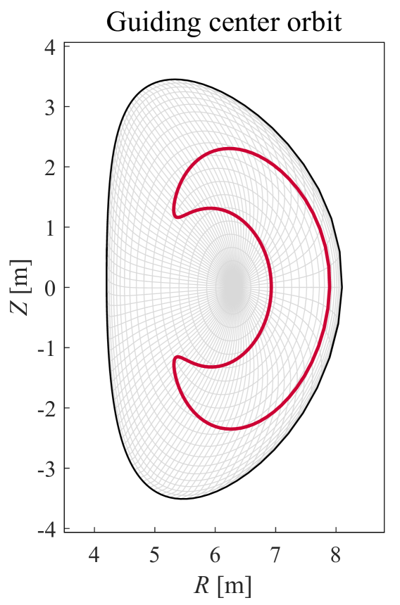
As input, FOX takes a file that contains all information characterizing the equilibrium configuration on a format compatible with Integrated Tokamak Modelling standards [18]. All scalar fields, such as , and , are specified on a grid in -space. The user defines an equidistant grid in -space, where all guiding center orbits are to be solved in the given equilibrium. Equation (6) is then solved for each on the grid by bilinear interpolation of in -space. An example of such a solution is shown in Fig. 2. The solution method is optimal for wide orbits, whereas thinner orbits require a large enough resolution of the equilibrium.
Once the guiding center orbit points are found in the poloidal plane, the time dependence of the orbit is calculated using eq. (9). Numerically, the integration is performed by assuming to be constant between adjacent points of the guiding center orbit. This assumption generates the approximation
| (39) |
where is the :th -point along the orbit and is evaluated at . Equation (39) becomes singular at the points where . Close to such a singularity, or when the -grid is coarse, large or even non-monotonous time coordinates may result. When these events are identified,111“Large” time steps are identified by FOX using the condition , where the constant . FOX successively eliminates points along the guiding center orbit until all time steps are small and monotonous. The coordinates of the orbit are then solved simply by using the trapezoidal method on eq. (12).
The eigenfunctions of the wave field, and the corresponding mode frequencies are solved by using the analytical approximations presented in Ref. [19]. Future versions of FOXTAIL intend to use the MHD eigenmode analyzer code MISHKA [20, 21, 22, 23] to solve the TAEs numerically. Besides ideal MHD effects, MISHKA also considers effects from finite ion Larmor radii, ion and electron drift, neoclassical ion viscosity and bootstrap current, indirect energetic ion effects and the collisionless skin effect. The interaction coefficients are calculated from eq. (24) on each point on the -grid also by using the trapezoidal method.
The user specifies which mode–Fourier coefficient pairs to be calculated by FOX. All bounce frequencies, precession frequencies, interaction coefficients, mode frequencies and toroidal mode numbers are then collected in a single output file. A separate output file is generated that contains all initial conditions used in a specific TAIL simulation, which contains the initial energetic particle distribution, flags on the mode–Fourier coefficient pairs to be active in the simulation, initial mode amplitudes, etc.
In the absence of collisions, the TAIL model equations of eq. (31) defines a system of ordinary differential equation, which is solved numerically using the standard 4th order Runge-Kutta method. When momentum diffusion is present, the model equations instead become a system of stochastic differential equations, which can be modeled numerically, e.g. by using an Itō–Taylor numerical scheme [24].
4 Numerical studies
4.1 Comparison with the 1D bump-on-tail model
One of the possible applications of FOXTAIL is to determine whether a one-dimensional bump-on-tail approximation of the system is sufficient to capture the essential wave–particle dynamics, such as growth rate and saturation amplitude. A higher computational efficiency typically follows from the lower dimensionality of the approximation. However, the 1D bump-on-tail model is only valid within certain parameter regimes. Section 4.1 presents a quantitative numerical study of these regimes.
4.1.1 Theoretical comparison
A simple bump-on-tail model, neglecting collisions, explicit wave damping and particle sources and sinks, can be written on the form [17]
| (40) |
where is the time coordinate, is the particle phase, is the particle momentum and is the complex eigenmode amplitude.
Now, consider the FOXTAIL model, only including a single mode and a single Fourier coefficient . We define the particle phase as
| (41) |
and the relative wave–particle frequency as
| (42) |
Next, we define a new momentum coordinate system , where both and
| (43) |
are constants of motion as particles move along the wave–particle characteristic curves of mode .
Assuming that the energetic particle distribution is located in a neighborhood around the wave–particle resonance (such that ) where and the interaction coefficient is constant in , the coordinate substitution
| (44) |
transforms the FOXTAIL model exactly to the 1D bump-on-tail model of eq. (40). Note that the substitutions of eq. (44) can be made for any FOXTAIL scenario, as long as one chooses a relevant eigenmode–Fourier coefficient pair and a resonant point .
According to the theory of the 1D bump-on-tail model, the linear growth rate of the mode () is [17]
| (45) |
where is the initial distribution function in . The growth rate in time can be approximated by
| (46) |
where is the distribution of energetic particles along the characteristic curves of wave–particle interaction (). In the 1D bump-on-tail model, particles deeply trapped by the wave field oscillate in -space around the resonance with the frequency222The frequency of eq. (47) is in real time, . For the frequency in the normalized time, , the expression should be multiplied by .
| (47) |
By comparing the numerical growth rates and other system properties of the 1D bump-on-tail model and FOXTAIL, one can make estimations of the effects of having non-constant and interaction coefficients, and of having multiple modes and/or Fourier coefficients.
4.1.2 Simulation parameters
In this study, we consider an ITER equilibrium configuration with an energetic particle distribution consisting of 3He2+ ions. For simplicity, we neglect collisions, explicit wave damping and particle sources and sinks. In such scenarios, the amplitudes of the modes are expected to grow exponentially until saturation at an amplitude proportional to the growth rate squared [25], assuming that the modes interact more or less independently with the energetic particle distribution. Since the magnetic moment is not a dynamical variable in this system, the dimensionality of the problem can be reduced by considering an energetic particle distribution on a surface. An ad hoc energetic particle distribution functions is constructed, with ( = ). The distribution in and are chosen to be Gaussians localized near the two resonances defined by and .
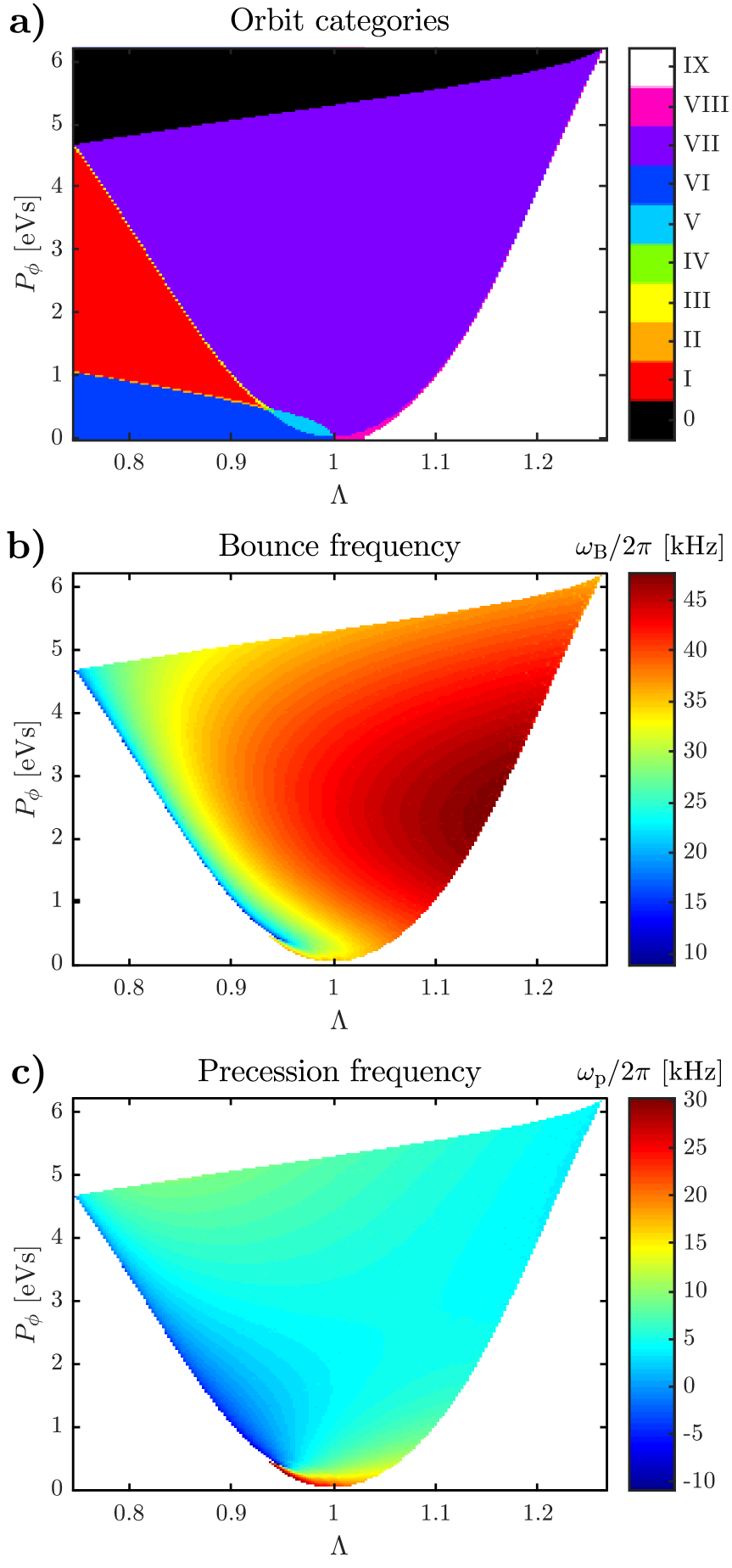
The chosen -grid to calculate the guiding center orbits is in the region of trapped particles (category V- and VII-orbits in Fig. 3.a) on the surface. The corresponding bounce and precession frequencies, presented in Figs. 3.b and 3.c, respectively, are found from the time dependence of the guiding center orbits, which are solved using eqs. (9) and (12).
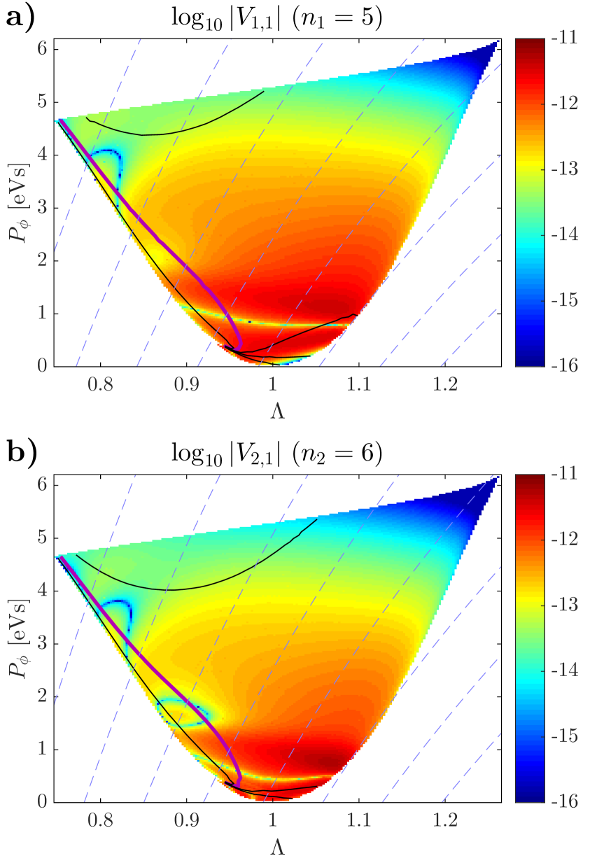
Two TAEs are chosen for this study: the first mode with a toroidal mode number , and the second one with . The energetic particle distribution is placed close to the resonance , i.e., the surface defined by , where is the frequency of the first TAE. Figure 4 shows the calculated interaction coefficients for , Fig. 4.a, and , Fig. 4.b. The frequencies of the two modes are and , respectively. Since the precession frequency is small compared to the bounce frequency at the resonance, the and the resonances are almost the same in -space.
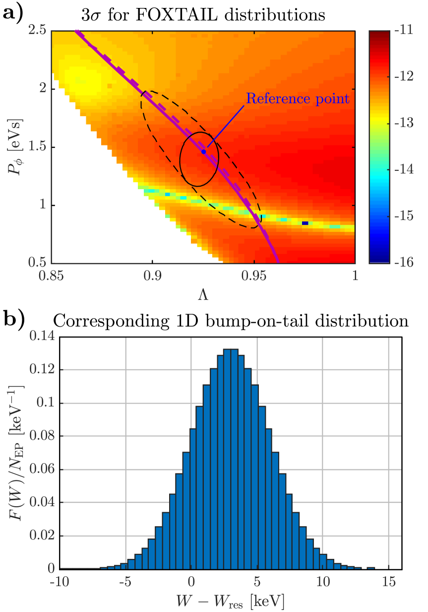
A reference point is chosen on the resonance, as shown in Fig. 5.a. Around this point, the bounce and precession frequencies are approximated to first order in -space, and is approximated to zeroth order, when transforming from the FOXTAIL to the 1D bump-on-tail coordinate system. Two different initial distribution functions are used in these studies: one localized around the reference point and one that is more spread along the resonance. The two distributions transform to the same distribution in the 1D bump-on-tail model, shown in Fig. 5.b. The initial distributions are chosen such that there is a positive derivative of the energy distribution at the resonance, giving a positive linear growth rate according to eq. (45).
An energetic particle distribution consisting of 3He2+ ions are distributed on markers. The markers are spread out in phase space using quasi-random low-discrepancy sequences (a Sobol’ sequence [27] combined with the Matoušek scrambling method [28]). They are placed as a Gaussian in -space centered around the resonance, and then the marker weights are set such that they represent the shifted Gaussian as in Fig. 5.b. This is done in order to improve the statistics of markers around the resonance as compared to a scenario with equal weights.
| Case | Eigenmodes | Fourier coefficients | [keV] | [keV] | factor | [kHz] | [] |
|---|---|---|---|---|---|---|---|
| #1 | 5.7 | 3.0 | 1 | 2.0 | 2.5 | ||
| #2 | 5.7 | 3.0 | – | – | 2.5 | ||
| #3 | 22.7 | 3.0 | 1 | 2.0 | 2.5 | ||
| #4 | 22.7 | 3.0 | – | – | 2.5 | ||
| #5 | 5.7 | 3.0 | 10.1 | 2.0 | 2.5 | ||
| #6 | 5.7 | 3.0 | 10.1 | – | 2.5 | ||
| #7 | 5.7 | 4.0 | – | – | 3.0 | ||
| #8 | 5.7 | 4.0 | 13.2 | 6.1 | 3.0 | ||
| #9 | 5.7 | 4.0 | 13.2 | – | 3.0 |
4.1.3 Numerical comparison with the 1D bump-on-tail model
Here, different FOXTAIL scenarios are compared with the corresponding 1D bump-on-tail scenario by varying initial parameters such as the width of the initial energetic particle distribution along the resonances and the number of eigenmodes and Fourier coefficients to include in the simulations. Besides the 1D scenario, four FOXTAIL scenarios are presented. In the first two scenarios (referred to as cases #1 and #2), a narrow initial distribution is used (see Fig. 5.a), whereas the two latter scenarios (cases #3 and #4) use the wide initial distribution. Furthermore, cases #1 and #3 include both of the TAEs presented in section 4.1.2 and a range of Fourier coefficients for both eigenmodes. Cases #2 and #4 only include the first eigenmode () and a single Fourier coefficient . For a complete list of initial parameter values used in the FOXTAIL simulations presented in this paper, see Table 1.
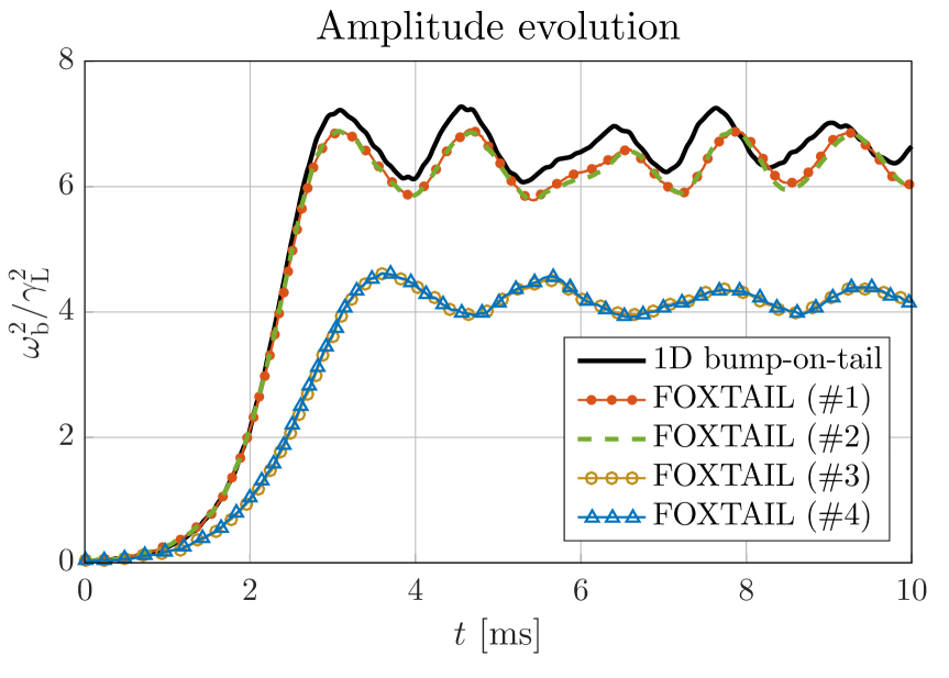
Figure 6 shows the amplitude evolutions of the first eigenmode for the bump-on-tail simulation and FOXTAIL simulations #1 – 4. The amplitude of the second mode never grows larger than 0.8 % of the amplitude of the first mode after saturation in case #1, and up to 5 % in case #3. It can immediately be seen that the two FOXTAIL scenarios with a narrow initial distribution (cases #1 and #2) agrees well with the corresponding 1D bump-on-tail scenario, both in growth rate and in saturation amplitude. On the other hand, the wider distribution (cases #3 and #4) gives a different growth rate and saturation level of the amplitude. This is presumably due to the fact that the wide distribution spans over regions where the interaction coefficient is considerably lower than in the reference point, giving a lower growth rate on average.
Including multiple eigenmodes and Fourier coefficients in the simulations seem to have negligible effects on the system in the considered scenarios, both for the narrow and the wide initial distributions. The reason for why the second mode does not influence the system considerably is because it has an expected growth rate of approximately 100 times lower than the first mode, which is due to the comparably lower values of the interaction coefficient in the region of the initial distribution function (recall that the growth rate scales as , see eq. (46)).
When comparing growth rates of the different scenarios, it should be noted that of the 1D bump-on-tail scenario is approximately 81 % of the analytical growth rate of eq. (45), whereas the growth rates of cases #1 and #2 are 77 % of the analytical growth rate, and 68 % for cases #3 and #4. The reason why the growth rate of the 1D bump-on-tail scenario is considerably lower than the analytical one is primarily because of the finite extension of the energetic particle distribution along the characteristic curves (this issue was analyzed in more detail in Ref. [17]).
4.2 Numerical multi-mode studies
The presence of multiple eigenmodes proved to have negligible effect on the system in the scenarios presented in section 4.1.3 due to the low interaction coefficient of the second mode in the considered part of -space, compared to the interaction coefficient of the first mode. Scenarios with significant multimode dynamics can be constructed by adding an ad hoc scaling factor to the interaction coefficient of the second mode. Multiplying by a factor of 10.1 gives approximately the same linear growth rate of the two modes. This has been done for cases #5 and #6, presented in Fig. 7, along with the previous case #2. The three scenarios are the same, except that in cases #2 and #6 the eigenmodes are simulated individually, whereas in case #5 both modes are included to the system. Such a comparison allows one to isolate the nonlinear effects of mode interaction via the energetic particle distribution.
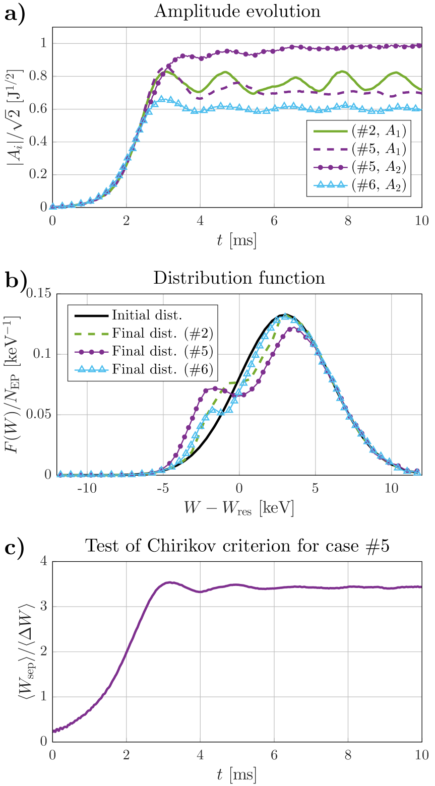
Comparing the multimode scenario with the scenarios where the modes are included individually, it can be seen that the indirect interaction between the modes via the energetic particles has significant macroscopic effects on the system. This can partly be understood as a consequence of stochastization of particle trajectories in phase space due to resonance overlap of the two eigenmodes. Stochastization of trajectories causes a locally enhanced transport of energetic particles around the resonances, allowing the eigenmodes to exhaust more energy from the energetic particle distribution (see e.g. stochastization from resonance overlap, [29, 30], and from phase decorrelation, [17]). This results in a wider portion of the energetic particle distribution being flattened around the resonances, compared to the individual eigenmode cases, as seen in Fig. 7.b.
The resonance width of an eigenmode can be estimated as the separatrix width of the unperturbed mode (i.e. in the absence of other modes) along the characteristic curve in -space, using the 1D bump-on-tail approximation. When the resonance widths of the two modes are comparable, the resonance-overlap parameter [31] (English translation: Ref. [32]), estimated as the average resonance width of the two modes divided by their distance in phase space, is an approximate measure of the level of stochastization of particle trajectories. The Chirikov criterion for stochastization is satisfied when the resonance-overlap parameter is larger than unity. The full separatrix width in -space, , is , with given by eq. (47). As seen in Fig. 7.c, the Chirikov criterion is well satisfied for case #5 after .
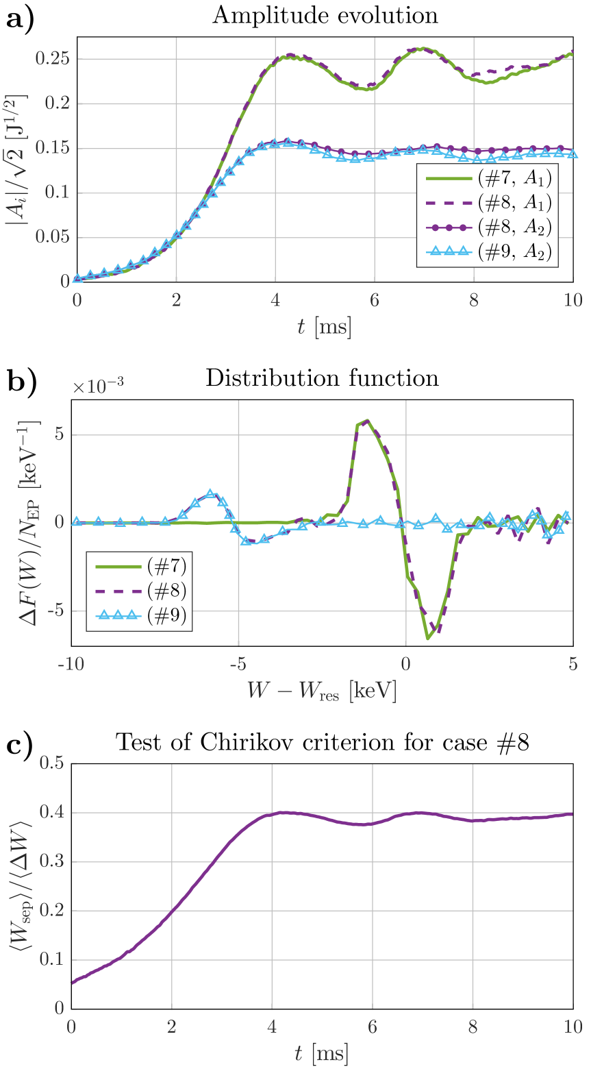
Slightly different scenarios are tested in the simulations presented in Fig. 8. Cases #7, #8 and #9 are the same as cases #2, #5 and #6, respectively, except that the frequency separation between the two eigenmodes is artificially increased by a factor of 3, and the width of the energetic distribution function along the characteristic curves of the first mode is increased to instead of . The scaling factor of the interaction coefficient is also adjusted such that the linear growth rates of the two modes approximately match. As can be seen in Fig. 8.c, the Chirikov criterion is never satisfied for case #8, although the resonance-overlap parameter is of the order of unity. Comparing the amplitude evolutions in Figs. 7.a and 8.a, the two modes of case #8 evolves more similarly to the corresponding individual mode scenarios than case #5 does. This is especially seen in Fig. 8.b, where the modes of case #8 flattens two separate regions of the energetic distribution function, matching the flattening regions of the individual mode scenarios.
5 Summary
This paper presents the theoretical framework of the FOXTAIL code, which is used to describe the nonlinear interaction between Alfvén eigenmodes and energetic particles in toroidal geometries. FOXTAIL is a hybrid magnetohydrodynamic–kinetic model based on a model developed by Berk et al. [4], where each simulation is formulated as an initial value problem. Eigenmodes are treated as perturbations of the equilibrium system, with temporally constant eigenfunctions and dynamic complex amplitudes that vary on time scales longer than the inverse mode frequency. The energetic particle distribution is modeled by a finite set of markers in an action–angle phase space of the unperturbed system. The use of action–angle coordinates rather than conventional toroidal coordinates simplifies the equations of motion of the individual markers, and it allows for efficient resolution of time scales relevant for resonant eigenmode–particle interaction in numerical simulations.
The particle response with respect to the wave field is quantized by a Fourier series expansion of the kinetic energy change along the transit period of the unperturbed guiding center orbit, where is the particle charge, is the guiding center velocity and is the electric wave field at the guiding center position. A Lagrangian formulation of the wave–particle system, consistent with the derived particle response with respect to the wave, is used to derive equations for the eigenmode amplitudes and phases. The resulting system of equations describing direct wave–particle interaction has a phase space with four particle dimensions and two eigenmode dimensions (amplitude and phase). When including mechanisms that perturb the magnetic moment of energetic particles, the particle phase space extends to five dimensions.
When splitting the interaction in the Fourier terms along the transit period, each term contributes to resonant nonlinear interaction mainly in a narrow region around surfaces in the adiabatic invariant space, referred to as resonant surfaces. These surfaces are given by , where is the Fourier index of interaction, is the bounce frequency, is the toroidal mode number of the eigenmode, is the precession frequency and is the eigenmode frequency. The width of the relevant region around the resonant surfaces depends on the amplitude of the eigenmode, the strength of wave–particle interaction at the resonant surfaces (quantified by the Fourier coefficients of interaction) and the variation of bounce and precession frequencies of particles along the characteristic curves of wave–particle interaction (the curves in adiabatic invariant space along which a given eigenmode accelerates particles).
The presented multi-dimensional model can be approximated with a conventional 1D bump-on-tail model. For the 1D approximation to be valid, three approximate criteria must be met:
-
1.
No more than one eigenmode–Fourier coefficient pair interacts significantly with the energetic particle distribution.
-
2.
The complex Fourier coefficient of interaction is approximately constant in adiabatic invariant space throughout the resonant part of the energetic particle distribution.
-
3.
The bounce and precession frequencies of the energetic particles vary approximately linearly in kinetic energy–toroidal canonical momentum space across the region of the resonance where the energetic particle distribution is located.
All these conditions can be quantitatively evaluated with FOXTAIL.
Effects of the fulfillment of the Chirikov criterion in scenarios with two active eigenmodes have been studied numerically using FOXTAIL. It has been verified that eigenmodes can be treated independently in scenarios where the criterion is not satisfied. On the other hand, when the resonance-overlap parameter becomes larger than unity, indirect mode–mode interaction via the energetic particle distribution becomes significant, and a larger portion of the inverted energetic particle distribution becomes flattened in energy space due to stochastization of particle trajectories in phase space.
Acknowledgments
This work was supported by the Swedish research council (VR) contract 621-2011-5387.
References
- [1] W. W. Heidbrink, E. J. Strait, E. Doyle, G. Sager, R. T. Snider, Nucl. Fusion 31 (9) (1991) 1635 – 1648. doi:10.1088/0029-5515/31/9/002.
- [2] K. L. Wong, R. J. Fonck, S. F. Paul, D. R. Roberts, E. D. Fredrickson, R. Nazikian, H. K. Park, M. Bell, N. L. Bretz, R. Budny, S. Cohen, G. W. Hammett, F. C. Jobes, D. M. Meade, S. S. Medley, D. Mueller, Y. Nagayama, D. K. Owens, E. J. Synakowski, Phys. Rev. Lett. 66 (14) (1991) 1874 – 1877. doi:10.1103/PhysRevLett.66.1874.
- [3] A. N. Kaufman, Phys. Fluids 15 (6) (1972) 1063 – 1069. doi:10.1063/1.1694031.
- [4] H. L. Berk, B. N. Breizman, M. S. Pekker, Nucl. Fusion 35 (12) (1995) 1713 – 1720. doi:10.1088/0029-5515/35/12/I36.
- [5] Z. Wang, Z. Lin, I. Holod, W. W. Heidbrink, B. Tobias, M. Van Zeeland, M. E. Austin, Phys. Rev. Lett. 111 (14) (2013) 145003. doi:10.1103/PhysRevLett.111.145003.
- [6] S. Briguglio, G. Vlad, F. Zonca, C. Kar, Phys. Plasmas 2 (10) (1995) 3711 – 3723. doi:10.1063/1.871071.
- [7] G. Vlad, C. Kar, F. Zonca, F. Romanelli, Phys. Plasmas 2 (2) (1995) 418 – 441. doi:10.1063/1.870968.
- [8] S. Briguglio, F. Zonca, G. Vlad, Phys. Plasmas 5 (9) (1998) 3287 – 3301. doi:10.1063/1.872997.
- [9] Z. Lin, T. S. Hahm, W. W. Lee, W. M. Tang, R. B. White, Science 281 (5384) (1998) 1835 – 1837. doi:10.1126/science.281.5384.1835.
- [10] W. Zhang, Z. Lin, L. Chen, Phys. Rev. Lett. 101 (9) (2008) 095001. doi:10.1103/PhysRevLett.101.095001.
- [11] Y. Xiao, Z. Lin, Phys. Rev. Lett. 103 (8) (2009) 085004. doi:10.1103/PhysRevLett.103.085004.
- [12] H. L. Berk, B. N. Breizman, M. S. Pekker, Plasma Phys. Rep. 23 (9) (1997) 778 – 788.
- [13] R. B. White, Phys. Fluids B 2 (4) (1009) 845 – 847. doi:10.1063/1.859270.
- [14] H. L. Berk, B. N. Breizman, J. Candy, M. Pekker, N. V. Petviashvili, Phys. Plasmas 6 (8) (1999) 3102 – 3113. doi:10.1063/1.873550.
- [15] M. K. Lilley, B. N. Breizman, S. E. Sharapov, Phys. Plasmas 17 (9) (2010) 092305. doi:10.1063/1.3486535.
- [16] L.-G. Eriksson, P. Helander, Phys. Plasmas 1 (2) (1994) 308 – 314. doi:10.1063/1.870832.
- [17] E. Tholerus, T. Hellsten, T. Johnson, Phys. Plasmas 22 (8) (2015) 082106. doi:10.1063/1.4928094.
- [18] F. Imbeaux, J. B. Lister, G. T. A. Huysmans, W. Zwingmann, M. Airaj, L. Appel, V. Basiuk, D. Coster, L.-G. Eriksson, B. Guillerminet, D. Kalupin, C. Konz, G. Manduchi, M. Ottaviani, G. Pereverzev, Y. Peysson, O. Sauter, J. Signoret, P. Strand, ITM-TF work programme contributors, Comput. Phys. Commun. 181 (6) (2010) 987 – 998. doi:10.1016/j.cpc.2010.02.001.
- [19] J. Candy, B. N. Breizman, J. W. Van Dam, T. Ozeki, Phys. Lett. A 215 (1996) 299 – 304. doi:10.1016/0375-9601(96)00197-1.
- [20] A. B. Mikhailovskii, G. T. A. Huysmans, W. O. K. Kerner, S. E. Sharapov, Plasma Phys. Rep. 23 (10) (1997) 844 – 857.
- [21] G. T. A. Huysmans, S. E. Sharapov, A. B. Mikhailovskii, W. Kerner, Phys. Plasmas 8 (10) (2001) 4292 – 4305. doi:10.1063/1.1398573.
- [22] S. E. Sharapov, A. B. Mikhailovskii, G. T. A. Huysmans, Phys. Plasmas 11 (5) (2004) 2286 – 2302. doi:10.1063/1.1690303.
- [23] I. T. Chapman, S. E. Sharapov, G. T. A. Huysmans, A. B. Mikhailovskii, Phys. Plasmas 13 (6) (2006) 062511. doi:10.1063/1.2212401.
- [24] P. E. Kloeden, E. Platen, Numerical Solution of Stochastic Differential Equations, Second Corrected Printing Edition, Vol. 23 of Applications of Mathematics, Springer-Verlag, Berlin, 1995, ISBN 978-3-540-54062-5.
- [25] M. B. Levin, M. G. Lyubarskiĭ, I. N. Onishchenko, V. D. Shapiro, V. I. Shevchenko, J. Exp. Theor. Phys. 35 (5) (1972) 898 – 901.
- [26] J. Hedin, T. Hellsten, L.-G. Eriksson, T. Johnson, Nucl. Fusion 42 (5) (2002) 527 – 540. doi:10.1088/0029-5515/42/5/305.
- [27] I. M. Sobol’, U.S.S.R. Comput. Maths. Math. Phys. 7 (4) (1967) 86 – 112. doi:10.1016/0041-5553(67)90144-9.
- [28] J. Matoušek, J. Complexity 14 (4) (1998) 527 – 556. doi:10.1006/jcom.1998.0489.
- [29] H. L. Berk, B. N. Breizman, H. Ye, Phys. Rev. Lett. 68 (24) (1992) 3563 – 3566. doi:10.1103/PhysRevLett.68.3563.
- [30] H. L. Berk, B. N. Breizman, M. Pekker, Phys. Plasmas 2 (8) (1995) 3007 – 3016. doi:10.1063/1.871198.
- [31] B. V. Chirikov, At. Energ. 6 (1959) 630 – 638.
- [32] B. V. Chirikov, J. Nucl. Energy, Pt. C 1 (1960) 253 – 260.