Fractality of profit landscapes and validation of time series models for stock prices
Abstract
We apply a simple trading strategy for various time series of real and artificial stock prices to understand the origin of fractality observed in the resulting profit landscapes. The strategy contains only two parameters and , and the sell (buy) decision is made when the log return is larger (smaller) than (). We discretize the unit square into the square grid and the profit is calculated at the center of each cell. We confirm the previous finding that local maxima in profit landscapes are scattered in a fractal-like fashion: The number of local maxima follows the power-law form , but the scaling exponent is found to differ for different time series. From comparisons of real and artificial stock prices, we find that the fat-tailed return distribution is closely related to the exponent observed for real stock markets. We suggest that the fractality of profit landscape characterized by can be a useful measure to validate time series model for stock prices.
pacs:
89.65.Gheconophysics, financial markets and 89.75.-kcomplex systems and 05.45.Dffractals1 Introduction
More and more physicists have been drawn to the research fields of economics and finance in the last few decades Stanleybook ; Bouchardbook ; Sinhabook . Those econophysicists brought new insights into such interdisciplinary area and developed useful analytical and computational tools. Many stylized facts in stock markets have been repeatedly discovered by researchers: the heavy tail in the return distribution, rapidly decaying autocorrelation of returns, the clustering and long-term memory of volatility, to list a few.
Recently, a geometric interpretation of the profit in stock markets has been proposed, in which the profit landscape of a stock has been constructed based on a simple virtual trading strategy Gronlund . Although the used trading strategy is too simple to mimic behaviors of real market traders, the simplicity has its own benefit: It allows us to construct the profit landscape in low dimensions and thus making the geometric analysis straightforward. More specifically, we use the two-parameter strategies to compute the long-term profit of individual stock in the real stock market. Our study in this paper is an extension of Ref. Gronlund : We first show that the observed fractality in Ref. Gronlund is a generic property of real stock markets, by examining stock markets in two different countries (Unites States and South Korea). We then pursue the origin of this observed fractality by applying the same methodology to various time series, real and artificial. It is revealed that the fractal structure in the profit landscapes in real markets is closely related with the existence of fat tails in the return distribution.
The present paper is organized as follows: In Sec. 2, we present the datasets we use and also describe briefly how we generate four different artificial time series to compare with real stock price movements. Our two-parameter trading strategy is also explained. Section 3 is devoted for the presentation of our results, which is followed by Sec. 4 for conclusion.
2 Methods
2.1 Time Series
In the present study, we employ a simple long-short trading strategy Gronlund and apply it to the historical daily real stock price time series as well as to artificially generated time series. For real historic stock prices, we use 526 stocks in South Korean (SK) for 10 years (Jan. 4, 1999 to Oct. 19, 2010), and 95 stocks in United States (US) for 21 years (Jan. 2, 1983 to Dec. 30, 2004). For SK dataset, the total number of trading days is , while for US. For artificially generated time series data, we use four different models that are widely used in fiance: the geometric Brownian motion (GBM), the fractional Brownian motion (FBM), the symmetric Lévy -stable process (LP), and the Markov-Switching Multifractal model (MSM). For each stochastic process, we generate 100 different time series for the same time period as for the SK dataset. In Table 1, we list the properties of different time series used in the present study.
| GBM | FBM | LP | MSM | Real Markets | |
|---|---|---|---|---|---|
| long-term memory | |||||
| heavy-tail distribution |

The GBM Black ; Hull is based on the stochastic differential equation
| (1) |
where is the price of stock and is the standard Brownian motion. For the drift and the volatility in Eq. (1), we use the values obtained from the SK dataset.
To mimic the existence of a long-term memory in real stock prices the continuous time stochastic process FBM has been introduced Mandelbrot , in which the covariance between the two stochastic processes and at time and satisfies
| (2) |
Here, the Hurst exponent plays an important role: For , FBM is the same as the standard Brownian motion, while for (), the increments of its stochastic process are positively (negatively) correlated. Accordingly, the long-term positive memory exists for . The long-term memory properties in various financial time series, such as stock indices, foreign exchange rates, futures, and commodity, have been found Ding ; Liu ; Cont ; Oh . In this work, we generate the process by using
| (3) |
where is the stochastic variable for the stock price and is the fractional Brownian motion [compare with Eq. (1)]. We use the package dvfBm in R-project to get the sample paths of FBM and generate time series for different values of the Hurst exponent .
We also generate the stochastic time series using LP Sinhabook ; Mantegna ; Pantaleo ; Schoutensbook ; Fusaibook , to imitate the heavy-tail distribution of return in real market (see Table 1). We first produce the stochastic process by LP and then generate the stock price Schoutensbook ; Applebaumbook via
| (4) |
LP contains the tunable parameter called the stability index which characterizes the shape of distribution. The distribution for the return converges to the Gaussian from as , while for it asymptotically exhibits the power-law behavior
| (5) |
for . Consequently, we can adjust the thickness of the tail part of the distribution by changing . We generate time series using LP for different values of .
MSM has been introduced to mimic the behaviors of real markets such as the heavy-tailed return distribution, the clustering of volatility, and so on MFbook ; Calvet2001 ; Calvet2004 (see Table 1). It has become the one of the most well accepted models in the area of finance and econometrics. To generate artificial stock prices based on MSM, we use
| (6) |
where is the log-return written as . The Gaussian random variable has zero mean and unit variance, and the volatility ) is constructed from the time series in MSM MFbook ; Calvet2001 ; Calvet2004 . In this work, we use the binomial MSM and use the parameter to generate different time series.
We generate artificial time series by using the above described four different models (GBM, FBM, LP, and MSM) and compare them with real market behavior in Fig. 1, which displays the stock price and the log-return time series in the left and the right columns, respectively. Qualitative difference between artificial time series [(b)-(e)] and the real price (a) is not easily seen. In contrast, the log-return shown in the right column of Fig. 1 exhibits a clear difference. In Fig 1(a) for the time series of the log-return for a real company in SK, one can recognize well-known stylized facts: Fluctuation of log-return around zero, called the volatility, has a broad range of sizes which implies the heavy-tailed return distribution. It is also seen that the volatility is clustered in time so that there is an active period of time when return fluctuates heavily and there is a calm period when return does not deviate much from zero. On the other hand, the two model time series GBM and FBM in Fig 1 (b) and (c) show somewhat different behavior: The size of fluctuation does not vary much, indicating the absence of the heavy tail in return distribution. In contrast, LP and MSM in Fig. 1 (d) and (e) exhibit the larger volatility fluctuation like the real market behavior in (a), indicating the heavy tail in return distribution. The difference between LP and real market can be seen in terms of the volatility clustering: In LP, the large volatility is not necessarily accompanied by other large volatility [Fig. 1(d)], whereas for MSM [Fig. 1(e)], and real market [Fig. 1(a)], volatility is often clustered in time.
2.2 Trading Strategy
In our simple trading strategy (see Ref. Gronlund for more details), the trade decision (buy or sell) is made when the log return with passes upper and lower boundaries: Sell for , buy for , and no trading if the log return remains within boundaries . As in Ref. Gronlund , we further parameterize the strategy by introducing the time lag defined by , the fraction of holding shares of stock when sell decision is made, and the fraction of cash in possession when buy.
We use the same notations as in Ref. Gronlund and call the above simple strategy as . In the inverse strategy Gronlund , buy (sell) decision is made for . It is interesting to see that is similar to the contrarian strategy (or trend-opposing strategy) and that to the momentum strategy (or trend-following strategy) Gronlund . However, we emphasize that the similarity is only superficial: The existence of trend has been strongly debated and in the area of econophysics the well-known absence of temporal correlation of the return is clearly against the existence of any trend in time scales longer than a couple of minutes Gopikrishnan .
The virtual trading strategy in this study is applied as follows:
-
1.
Start with one billion Korean Won () at as initial amount of investment. 111The exchange rate between US Dollar and Korean Won (KRW) is about .
-
2.
Pick a company .
-
3.
For a given parameter pair (), keep applying the trading strategy, or , until the last trading day . For each trading, the amount of cash and the number of stocks change.
At the end of the trading period , we assess the total value of our virtual portfolio as the sum of cash and the stock holdings: . The performance of the strategy is evaluated by the ratio between the net profit and the initial investment, i.e.,
| (7) |
We constrain that the lower bound of cash is zero, i.e., , and that the number of shares is non-negative, i.e, . For the sake of simplicity, we also assume that the market price of stock is the same as the daily closing price in the historic data, and the transaction commission fee is taken into account for every trading.
3 Results
3.1 Real time series
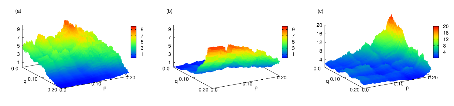
We calculate the profit of each strategy for the -th company in order to study the fractality of profit landscape in stock markets. The unit square in - plane is discretized by the resolution parameter so that it contains small squares of the size . The shape of the profit landscape not only differs from company to company but also depends on the details of strategy such as the values of , and time lags as seen in Fig. 2 for two companies in SK: Samsung Electronics and Hyundai Motors. We also find that the shape of the profit landscape and the locations of maxima and minima totally change for different time interval , , and Gronlund . Even if the shape of the profit landscape looks quite different for various parameter and different time interval, it is revealed that the nature of profit landscape does not change through Ref. Gronlund .
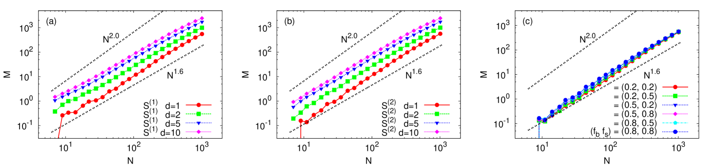
Once we get for a given resolution , we count the number of local maxima, where the profit is larger than profits for its von Neumann neighborhood (the four nearest cells surrounding the central cell). Apparently, must be an increasing function of , but how it depends on can be an interesting question to pursue. As is already observed for US stocks Gronlund , we again confirm that with as shown in Fig. 3, where is obtained from the average over 526 stocks in SK. Our finding of the same exponent both for US and SK indicates that the fractality of the profit landscape can be of a universal feature of different stock markets. We also check the robustness of the exponent for different values of the parameters. Figure 3 (a) and (b) show that the same scaling relation holds regardless of the specific strategy and different time lags . Figure 3 (c) confirms again for various parameter combinations of (, ). Although not shown here, is again obtained when we use the Moore neighborhood (the eight cells surrounding the central cell) instead of the von Neumann neighbors, and when the size of parameter set is expanded to . These results seem to suggest that the fractal nature of the profit landscape is a genuine feature of the real stock markets.
Although the trading strategies employed in this work might be too simple to be used in reality, we believe that a complicated trading strategy can be decomposed into a time-varying sophisticated mixture of simple strategies like and . Our observation of the robustness of the fractality suggests that more realistic strategies beyond those used here must also have complicated profit landscape, which is expected to exhibit a fractal characteristic.
3.2 Artificial time series
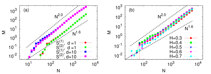
We repeat the above procedure to construct profit landscapes for four different artificial time series models GBM, FBM, LP, and MSM (see Sec. 2). Figure 4 shows versus for (a) GBM and (b) FBM. Interestingly, we again find the scaling form but with for both GBM and FBM, which is significantly different from observed in real markets. It is to be noted that the value indicates that the local maxima in the profit landscapes for GBM and FBM are scattered like two-dimensional objects. Also observed is that the scaling exponent does not change much as the Hurst exponent is varied in FBM as shown in Fig. 4(b). This is a particularly interesting result since FBM with is known to have the long-term memory effect like real markets. The difference of between real markets and FBM implies that the nontrivial value in real markets may not originate from the long-term memory effect.
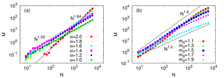
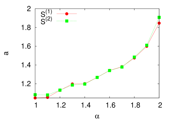
We next construct profit landscapes for LP and MSM and measure the scaling exponents in Fig. 5(a) and (b), respectively. For LP, the stability index controls the shape of the return distribution as described in Sec. 2. As is decreased from the Gaussian limit , the tail part of the return distribution becomes thicker. In Fig. 5(a), it is clearly shown that the scaling exponent which characterizes the fractality of the distribution of the local maxima in the profit landscapes changes in a systematic way with . It starts from the Gaussian limit value [compare with Fig. 4(a) for GBM] when and systematically decreases toward , as displayed in Fig. 6. Note also that and do not display any significant difference in Fig. 6. Consequently, it is tempting to conclude that the shape of the tail part of the return distribution (controlled by in LP) determines the scaling exponent in the profit landscape. When , we get as for the real markets. In Table 1, MSM is also shown to have the heavy tail in return distribution. From the study of LP, one can expect that MSM should also lead to as for LP. Figure 5(b) displays that a proper choice of the parameter in MSM gives us . Another interesting observation one can make from our MSM study is that appears to be an maximum value one can have, and the reason for this behavior needs to be sought in a future study.
In order to isolate the effects of the fat-tailed return distribution from the long-term memory effects, we generate the time series of returns and fully shuffle them in time to produce a new stock price time series. In this shuffling process, all existing long-time correlations are destroyed, but the probability distribution of returns remains intact. We apply this method for real stocks and the MSM time series, and compute . Although not shown here, we find that the scaling exponent remains the same, which again indicates that the fractal nature of the profit landscapes hardly depends on the existence of long-term memory, as was already found for the LP.
4 Conclusion
In summary, we have investigated the origin of the fractality of the profit landscape in two different real markets in comparison with four different models for generating artificial time series. The number of local maxima has been shown to scale with the resolution parameter following the form . Although the real markets exhibit , time series models with the short-tailed return distributions (GBM and FBM) fail to produce this scaling exponent. In contrast, the two different model time series (LP and MSM) have been shown to give us the scaling exponent consistent with market value . In LP, a systematic tuning of the thickness of the tail part of the return distribution has led to the main conclusion of the present work: The origin of fractality in the profit landscape is the heavy-tail of the return distribution. We suggest that the observed fractality of the profit landscape with the exponent can play an important role in validation procedure of artificial time series models for stock prices. In particular, one can tune the model parameters ( in LP and in MSM, for example) to make the time series compatible with the observed fractality in real markets.
Acknowledgements.
B. J. K. (Grant No. 2011-0015731) and G. O. (Grant No. 2012-0359) acknowledge the support from the National Research Foundation of Korea (NRF) grant funded by the Korea government (MEST).References
- (1) R. N. Mantegna and H. E. Stanley, An Introduction to Econophysics (Cambridge University Press, Cambridge, 2000).
- (2) J. P. Bouchard and M. Potters, Theory of Financial Risk and Derivative Pricing (Cambridge University Press, Cambridge, 2009).
- (3) S. Sinha, A. Chatterjee, A. Chakraborti, B. K. Chakrabarti, Econophysics: An Introduction (Wiley-VCH, Weinheim, 2010).
- (4) A. Grönlund, I. G. Yi, and B. J. Kim, PLoS ONE 7, e33960 (2012).
- (5) F. Black, The Journal of Political Economy 81, 637 (1973).
- (6) J. C. Hull, Options, Futures, and Other Derivatives (Pearson Education Ltd., London, 2009).
- (7) B. b. Mandelbrot and J. W. Van Ness, SIAM review 10, 422 (1968).
- (8) Z. Ding, C. W. J. Granger, and R. F. Engle, Journal of Empirical Finance 1, 83 (1993).
- (9) Y. Liu, P. Gopikrishnan, P. Cizeau, M. Meyer, -C. -K. Peng, and H. E. Stanley, Phys. Rev. E 60, 1390 (1999).
- (10) R. Cont, Quantitative Finance 1, 223 (2001).
- (11) G. Oh and S. Kim, J. Korean Phys. Soc. 48, S197 (2006).
- (12) R. N. Mantegna, Phys. Rev. E 49, 4677 (1994).
- (13) E. Pantaleo, P. Facchi, and S. Pascazio, Physica Scripta T135, 014036 (2009).
- (14) W. Schoutens, Lévy process in Finance (John Wiley & Sons Ltd., New York, 2003).
- (15) G. Fusai and A. Roncoroni, Implementing Models in Quantitative Finance: Methods and Cases (Springer-Verlag, Berlin, 2008).
- (16) D. Applebaum, Lévy Processes and Stochastic Calculus (Cambridge University Press, Cambridge, 2009).
- (17) L. E. Calvet and A. J. Fisher, Multifractal Volatility (Academic Press, Burlington, 2008).
- (18) L. E. Calvet and A. J. Fisher, Journal of Econometrics 105, 27 (2001).
- (19) L. E. Calvet and A. J. Fisher, Journal of Financial Econometrics 2, 49 (2004).
- (20) P. Gopikrishnan, V. Plerou, L. A. N. Amaral, M. Meyer, and H. E. Stanley, Phys. Rev. E 60, 5305 (1999).