Fractals with point impact in functional linear regression
Abstract
This paper develops a point impact linear regression model in which the trajectory of a continuous stochastic process, when evaluated at a sensitive time point, is associated with a scalar response. The proposed model complements and is more interpretable than the functional linear regression approach that has become popular in recent years. The trajectories are assumed to have fractal (self-similar) properties in common with a fractional Brownian motion with an unknown Hurst exponent. Bootstrap confidence intervals based on the least-squares estimator of the sensitive time point are developed. Misspecification of the point impact model by a functional linear model is also investigated. Non-Gaussian limit distributions and rates of convergence determined by the Hurst exponent play an important role.
doi:
10.1214/10-AOS791keywords:
[class=AMS] .keywords:
.and
t1Supported by NSF Grant DMS-08-06088. t2Supported by NSF Grant DMS-09-06597.
1 Introduction
This paper investigates a linear regression model involving a scalar response and a predictor given by the value of the trajectory of a continuous stochastic process , at some unknown time point. Specifically, we consider the point impact linear regression model
| (1) |
and focus on the time point as the target parameter of interest. The intercept and the slope are scalars, and the error is taken to be independent of , having zero mean and finite variance . The complete trajectory of is assumed to be observed (at least on a fine enough grid that it makes no difference in terms of accuracy), even though the model itself only involves the value of at , which represents a “sensitive” time point in terms of the relationship to the response. The main aim of the paper is to show that the precision of estimation of is driven by fractal behavior in , and to develop valid inferential procedures that adapt to a broad range of such behavior. Our model could easily be extended in various ways, for example, to allow multiple sensitive time points or further covariates, but, for simplicity, we restrict attention to (1).
Our motivation for developing this type of model arises from genome-wide expression studies that measure the activity of numerous genes simultaneously. In these studies, it is of interest to locate genes showing activity that is associated with clinical outcomes. Emilsson et al. emilsson , for example, studied gene expression levels at over 24,000 loci in samples of adipose tissue to identify genes correlated with body mass index and other obesity-related outcomes. Gruvberger-Saal et al. gruvberger used gene expression profiles from the tumors of breast cancer patients to predict estrogen receptor protein concentration, an important prognostic marker for breast tumors; see also buness . In such studies, the gene expression profile across a chromosome can be regarded a functional predictor, and a gene associated with the clinical outcome is identified by its base pair position along the chromosome; see Figure 1. Our aim here is to develop a method of estimating a confidence interval for , leading to the identification of chromosomal regions that are potentially useful for diagnosis and therapy. Although there is extensive statistical literature on gene expression data, it is almost exclusively concerned with multiple testing procedures for detecting differentially expressed genes; see, for example, dula , salas .
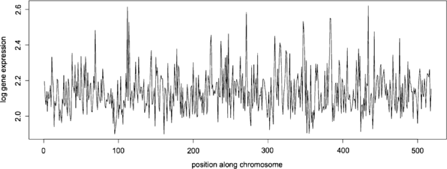
Gene expression profiles (as in Figure 1) clearly display fractal behavior, that is, self-similarity over a range of scales. Indeed, fractals often arise when spatiotemporal patterns at higher levels emerge from localized interactions and selection processes acting at lower levels, as with gene expression activity. Moreover, the recent discovery l-a that chromosomes are folded as “fractal globules,” which can easily unfold during gene activation, also helps explain the fractal appearance of gene expression profiles.
A basic stochastic model for fractal phenomena is provided by fractional Brownian motion (fBm) (see manness ), in which the so-called Hurst exponent calibrates the scaling of the self-similarity and provides a natural measure of trajectory roughness. It featured prominently in the pioneering work of Benoît Mandelbrot, who stated (man , page 256) that fBm provides “the most manageable mathematical environment I can think of (for representing fractals).” For background on fBm from a statistical modeling point of view, see gn .
The key issue to be considered in this paper is how to construct a confidence interval for the true sensitive time point based on its least squares estimator , obtained by fitting model (1) from a sample of size ,
| (2) |
We show that, when is fBm, both the rate of convergence and limiting distribution of depend on . In addition, we construct bootstrap confidence intervals for that do not require knowledge of . This facilitates applications (e.g., to gene expression data) in which the type of fractal behavior is not known in advance; the trajectory in Figure 1 has an estimated Hurst exponent of about 0.1, but it would be very difficult to estimate precisely using data in a small neighborhood of , so a bootstrap approach becomes crucial. We emphasize that nothing about the distribution of is used in the construction of the estimators or the bootstrap confidence intervals; the fBm assumption will only be utilized to study the large sample properties of these procedures. Moreover, our main results will make essential use of the fBm assumption only locally, that is, in a small neighborhood of .
The point impact model (1) can be regarded as a simple working model that provides interpretable information about the influence of at a specific location (e.g., a genetic locus). Such information cannot be extracted using the standard functional linear regression model rs given by
| (3) |
where is a continuous function and is an intercept, because the influence of is spread continuously across and point-impact effects are excluded. In the gene expression context, if only a few genes are predictive of , then a model of the form (1) would be more suitable than (3), which does not allow to have infinite spikes. In general, however, a continuum of locations is likely to be involved (as well as point-impacts), so it is of interest to study the behavior of in misspecified settings in which the data arise from combinations of (1) and (3).
Asymptotic results for the least squares estimator (2) in the correctly specified setting are presented in Section 2. In Section 3 it is shown that the residual bootstrap is consistent for the distribution of , leading to the construction of valid bootstrap confidence intervals without knowing . The nonparametric bootstrap is shown to be inconsistent in the same setting. The effect of misspecification is discussed in Section 4. A two-sample problem version of the point impact model is discussed in Section 5. Some numerical examples are presented in Section 6, where we compare the proposed bootstrap confidence interval with Wald-type confidence intervals (in which is assumed to be known); an application to gene expression data is also discussed. Concluding remarks appear in Section 7. Proofs are placed in Section 8.
2 Least squares estimation of the sensitive time point
Throughout we take to be a fBm with Hurst exponent , which, as discussed earlier, controls the roughness of the trajectories. We shall see in this section that the rate of convergence of can be expressed explicitly in terms of .
First we recall some basic properties of fBm. A (standard) fBm with Hurst exponent is a Gaussian process , having continuous sample paths, mean zero and covariance function
| (4) |
By comparing their mean and covariance functions, as processes, for all (self-similarity). Clearly, is a two-sided Brownian motion, and is a random straight line: where . The increments are negatively correlated if , and positively correlated if . Increasing results in smoother sample paths.
Suppose , are i.i.d. copies of satisfying the model (1). The unknown parameter is , and its true value is denoted . The following conditions are needed:
-
[(A3)]
-
(A1)
is a fBm with Hurst exponent .
-
(A2)
and .
-
(A3)
for some .
The construction of the least squares estimator , defined by (2), does not involve any assumptions about the distribution of the trajectories, whereas the asymptotic behavior does. Our first result gives the consistency and asymptotic distribution of under the above assumptions.
Theorem 2.1
If (A1) and (A2) hold, then is consistent, that is, . If (A3) also holds, then
where and are i.i.d. , independent of the fBm .
Remarks
-
1.
It may come as a surprise that the convergence rate of increases as decreases, and becomes arbitrarily fast as . A heuristic explanation is that fBm “travels further” with a smaller , so independent trajectories of are likely to “cover different ground,” making it easier to estimate . In a nutshell, the smaller the Hurst exponent, the better the design.
-
2.
It follows from (a sight extension of) Lemmas 2.5 and 2.6 of Kim and Pollard kp that the third component of is well defined.
-
3.
Using the self-similarity of fBm, the asymptotic distribution of can be expressed as the distribution of
(6) This distribution does not appear to have been studied in the literature except for and (standard normal). When , is a standard Brownian motion and the limiting distribution is given in terms of a two-sided Brownian motion with a triangular drift. Bhattacharya and Brockwell bb showed that this distribution has a density that can be expressed in terms of the standard normal distribution function. It arises frequently in change-point problems under contiguous asymptotics y , s , ms .
-
4.
From the proof, it can be seen that the essential assumptions on are the self-similarity and stationary increments properties in some neighborhood of , along with the trajectories of being Lipschitz of all orders less than . Note that any Gaussian self-similar process with stationary increments and zero mean is a fBm (see, e.g., Theorem 1.3.3 of em ).
-
5.
The trajectories of fBm are nondifferentiable when , so the usual technique of Taylor expanding the criterion function about does not work and a more sophisticated approach is required to prove the result.
-
6.
Note that has the same limiting behavior as though is known, and and are asymptotically independent.
-
7.
The result is readily extended to allow for additional covariates [cf. (11)], which is often important in applications. The limiting distribution of remains the same, and the other regression coefficient estimates have the same limiting behavior as though is known.
-
8.
Note that the assumption is crucial for the theorem to hold. When , the fBm does not influence the response at all and contains no information about .
3 Bootstrap confidence intervals
In general, a valid Wald-type confidence interval for would at least need a consistent estimator of the Hurst exponent , which is a nuisance parameter in this problem. Unfortunately, however, accurate estimation of is difficult and quite often unstable. Bootstrap methods have been widely applied to avoid issues of nuisance parameter estimation, and they work well in problems with -rates; see bickel81 , singh81 , shao95 and the references therein. In this section we study the consistency properties of two bootstrap methods that arise naturally in our setting. One of these methods leads to a valid confidence interval for without requiring any knowledge of .
3.1 Preliminaries
We start with a brief review of the bootstrap. Given a sample from an unknown distribution , suppose that the distribution function, , say, of some random variable , is of interest; is usually called a root and it can in general be any measurable function of the data and the distribution . The bootstrap method can be broken into three simple steps: {longlist}
Construct an estimator of from .
Generate given .
Estimate by , the conditional c.d.f. of given . Let denote the Lévy metric or any other metric metrizing weak convergence of distribution functions. We say that is weakly consistent if ; if has a weak limit , this is equivalent to converging weakly to in probability.
The choice of mostly considered in the literature is the empirical distribution. Intuitively, an that mimics the essential properties (e.g., smoothness) of the underlying distribution can be expected to perform well. In most situations, the empirical distribution of the data is a good estimator of , but in some nonstandard situations it may fail to capture some of the important aspects of the problem, and the corresponding bootstrap method can be suspect. The following discussion illustrates this phenomenon (the inconsistency when bootstrapping from the empirical distribution of the data) when is the random variable of interest.
3.2 Inconsistency of bootstrapping pairs
In a regression setup there are two natural ways of bootstrapping: bootstrapping pairs (i.e., the nonparametric bootstrap) and bootstrapping residuals (while keeping the predictors fixed). We show that bootstrapping pairs (drawing data points with replacement from the original data set) is inconsistent for .
Theorem 3.1
Under conditions (A1)–(A3), the nonparametric bootstrap is inconsistent for estimating the distribution of , that is, , conditional on the data, does not converge in distribution to in probability, where is defined by (6).
3.3 Consistency of bootstrapping residuals
Another bootstrap procedure is to use the form of the assumed model more explicitly to draw the bootstrap samples: condition on the predictor and generate its response as
| (7) |
where the are conditionally i.i.d. under the empirical distribution of the centered residuals , with and . Let and be the estimates of the unknown parameters obtained from the bootstrap sample. We approximate the distribution of [see (2.1)] by the conditional distribution of
given the data.
Theorem 3.2
Under conditions (A1)–(A3), the above procedure of bootstrapping residuals is consistent for estimating the distribution of , that is, , in probability, conditional on the data.
We now use the above theorem to construct a valid confidence interval (CI) for that does not require any knowledge of . Let be the -quantile of the conditional distribution of given the data, which can be readily obtained via simulation and does not involve the knowledge of any distributional properties of . The proposed approximate -level bootstrap CI for is then given by
Under the assumptions of Theorem 3.2, the coverage probability of this CI is
where denotes the bootstrap distribution given the data, and we have used the fact that the supremum distance between the relevant distribution functions of and is asymptotically negligible. The key point of this argument is that and have the same normalization factor and, thus, it “cancels” out. CIs for and can be constructed in a similar fashion.
3.4 Discussion
In nonparametric regression settings, dichotomies in the behavior of different bootstrap methods are well known, for example, when using the bootstrap to calibrate omnibus goodness-of-fit tests for parametric regression models; see hm , vkgms , neu and references therein. A dichotomy in the behavior of the two bootstrap methods, however, is surprising in a linear regression model. This illustrates that in problems with nonstandard asymptotics, the usual nonparametric bootstrap might fail, whereas a resampling procedure that uses some particular structure of the model can perform well. The improved performance of bootstrapping residuals will be confirmed by our simulation results in Section 6.
The difference in the behavior of the two bootstrap methods can be explained as follows. As in any M-estimation problem, the standard approach is to study the criterion (objective) function being optimized, in a neighborhood of the target parameter, by splitting it into an empirical process and a drift term. The drift term has different behavior for the two bootstrap methods: while bootstrapping pairs, it does not converge, whereas the bootstrapped residuals are conditionally independent of the predictors, and the drift term converges. This highlights the importance of designing the bootstrap to accurately replicate the structure in the assumed model. A more technical explanation is provided in a remark following the proof of Theorem 3.2.
Other types of resampling (e.g., the -out-of- bootstrap, or subsampling) could be applicable, but such methods require knowledge of the rate of convergence, which depends on the unknown . Also, these methods require the choice of a tuning parameter, which is problematic in practice. However, the residual bootstrap is consistent, easy to implement, and does not require the knowledge of and the estimation of a tuning parameter.
The inconsistency of the nonparametric bootstrap casts some doubt on its validity for checking the stability of variable selection results in high-dimensional regression problems (as is common practice). Indeed, it suggests that more care (in terms of more explicit use of the model) is needed in the choice of a bootstrap method in such settings.
4 Misspecification by a functional linear model
The point impact model cannot capture effects that are spread out over the domain of the trajectory, for example, gene expression profiles for which the effect on a clinical outcome involves complex interactions between numerous genes. Such effects, however, may be represented by a functional linear model, and we now examine how the limiting behavior of changes when the data arise in this way.
4.1 Complete misspecification
In this case we treat (1) as the working model (for fitting the data), but view this model as being completely misspecified in the sense that the data are generated from the functional linear model (3). For simplicity, we set and in the working model, and set in the true functional linear model. The least squares estimator now estimates the minimizer of
and the following result gives its asymptotic distribution.
Theorem 4.1
Suppose that (A1) and (A3) hold, and that has a unique minimizer and is twice-differentiable at . Then, in the misspecified case,
where and .
Remarks
-
1.
Here the rate of convergence reverses itself from the correctly specified case: the convergence rate now decreases as decreases, going from a parametric rate of when , to as slow as as . A heuristic explanation is that roughness in now amounts to measurement error (which results in a slower rate) as the fluctuations of are smoothed out in the true model.
-
2.
In the case of Brownian motion trajectories (), note that , the normal equation is
(8) and .
-
3.
Also in the case , the limiting distribution is given in terms of two-sided Brownian motion with a parabolic drift, and was investigated originally by Chernoff c in connection with the estimation of the mode of a distribution, and shown to have a density (as the solution of a heat equation). The Chernoff distribution arises frequently in monotone function estimation settings; Groeneboom and Wellner gw introduced various algorithms for computation of its distribution function and quantiles.
4.2 Partial misspecification
The nonparametric functional linear model (3) can be combined with (1) to give the semiparametric model
| (9) |
which allows to have both a point impact and an influence that is spread out continuously in time. When , this model reduces to the point impact model; when , to the functional linear model. In this section we examine the behavior of when the working model is (1), as before, but the data are now generated from (9).
For simplicity, suppose that and in both the working point impact model and in the true model (9). Denote the true value of by . It can then be shown that is robust to small levels of misspecification, that is, it consistently estimates with the same rate of convergence as in the correctly specified case. Indeed, targets the minimizer of the criterion function
Provided is sufficiently small, the derivative of will be negative over the interval and positive over , so is minimized at . It is then possible to extend Theorem 2.1 to give
| (10) |
where is defined in the statement of Theorem 4.1. This shows that the effect of partial misspecification is a simple inflation of the variance [cf. (6)], without any change in the form of the limit distribution.
It is also of interest to estimate in a way that adapts to any function (i.e., sufficiently smooth) in this semiparametric setting. This could be done, for example, by approximating by a finite B-spline basis expansion of the form , and fitting the working model
| (11) |
where are additional covariates with regression coefficients ; the resulting least squares estimator can then be used as an estimate of of . For the working model (11), the misspecification is , which will be small if is sufficiently large. Therefore, based on our previous discussion, will satisfy a result of the form (10); in particular, will exhibit the fast -rate of convergence. Note that for this result to hold, can be fixed and does not need to tend to infinity with the sample size.
5 Two-sample problem
In this section we discuss a variation of the point impact regression model in which the response takes just two values (say ). This is of interest, for example, in case-control studies in which gene-expression data are available for a sample of cancer patients and a sample of healthy controls, and the target parameter is the locus of a differentially expressed gene.
Suppose we have two independent samples of trajectories , with trajectories from class 1, and trajectories from class , for a total sample size of . It is assumed that remains fixed, and the th sample satisfies the model
where , are i.i.d. fBms with Hurst exponent , and is an unknown mean function, assumed to be continuous. The treatment effect is taken to have a point impact in the sense of having a unique maximum at ; minima can of course be treated in a similar fashion. The least squares estimator of the sensitive time point now becomes
| (12) |
where is the sample mean for class . Although a studentized version (normalizing the the difference of the sample means by a standard error estimate) might be preferable in some cases, with small or unbalanced samples, say, to keep the discussion simple, we restrict attention to . The empirical criterion function converges uniformly to a.s. (by the Glivenko–Cantelli theorem), so is a consistent estimator of .
As before, our objective is to find a confidence interval for based on under appropriate conditions on the treatment effect. Toward this end, we need an assumption on the degree of smoothness of the treatment effect at in terms of an exponent :
as , where . If is twice-differentiable at , then this assumption holds only with ; for it to hold for some , a cusp is needed. When the smoothness of the treatment effect and the fBm match, that is, , the rate of convergence of is , as before, and has a nondegenerate limit distribution of the same form as in Theorem 2.1:
| (13) |
The key step in the proof (which is simpler than in the regression case) is given at the end of Section 8.
6 Numerical examples
In this section we report some numerical results based on trajectories from fBm simulations and from gene expression data.
We first consider a correctly specified example as in Section 2 and study the behavior of CIs for the sensitive time-point using the two bootstrap based methods, and compare them with the Wald-type CI
| (14) |
with assumed to be known. Here is the sample standard deviation of the residuals, and is the upper -quantile of . In practice, needs to be estimated to apply (14). Numerous estimators of based on a single realization of have been proposed in the literature b , coeur , although observation at fine time scales is required for such estimators to work well, and it is not clear that direct plug-in would be satisfactory. The quantiles needed to compute the Wald-type CIs were extracted from an extensive simulation of the limit distribution, as no closed form expression is available.
Table 1 reports the estimated coverage probabilities and average lengths of nominal 95% confidence intervals for calculated using 500 independent samples. The data were generated from the model (1), for , , , where and , the Hurst exponent and sample sizes and . To calculate the least squares estimators (2), we restricted to a uniform grid of 101 points in ; the fBm trajectories were generated over the same grid. The fBm simulations were carried out in R, using the function fbmSim from the fArma package, and via the Cholesky method of decomposing the covariance matrix of . Histograms and scatterplots of and for when are displayed in Figure 2.
| Wald- | R bootstrap | NP bootstrap | ||||||
|---|---|---|---|---|---|---|---|---|
| Cover | Width | Cover | Width | Cover | Width | |||
| 20 | 0.3 | 0.3 | 0.874 | 0.023 | 0.924 | 0.044 | 1.000 | 0.174 |
| 0.5 | 0.880 | 0.088 | 0.946 | 0.119 | 0.992 | 0.220 | ||
| 0.7 | 0.822 | 0.170 | 0.912 | 0.249 | 0.970 | 0.360 | ||
| 0.5 | 0.3 | 0.806 | 0.129 | 0.912 | 0.211 | 0.998 | 0.410 | |
| 0.5 | 0.852 | 0.256 | 0.924 | 0.333 | 0.988 | 0.487 | ||
| 0.7 | 0.834 | 0.352 | 0.938 | 0.510 | 0.962 | 0.591 | ||
| 40 | 0.3 | 0.3 | 0.984 | 0.007 | 0.986 | 0.002 | 1.000 | 0.022 |
| 0.5 | 0.892 | 0.048 | 0.942 | 0.053 | 0.992 | 0.087 | ||
| 0.7 | 0.898 | 0.108 | 0.930 | 0.138 | 0.976 | 0.182 | ||
| 0.5 | 0.3 | 0.900 | 0.039 | 0.928 | 0.054 | 0.998 | 0.149 | |
| 0.5 | 0.908 | 0.134 | 0.950 | 0.165 | 0.990 | 0.251 | ||
| 0.7 | 0.856 | 0.229 | 0.946 | 0.332 | 0.962 | 0.386 | ||
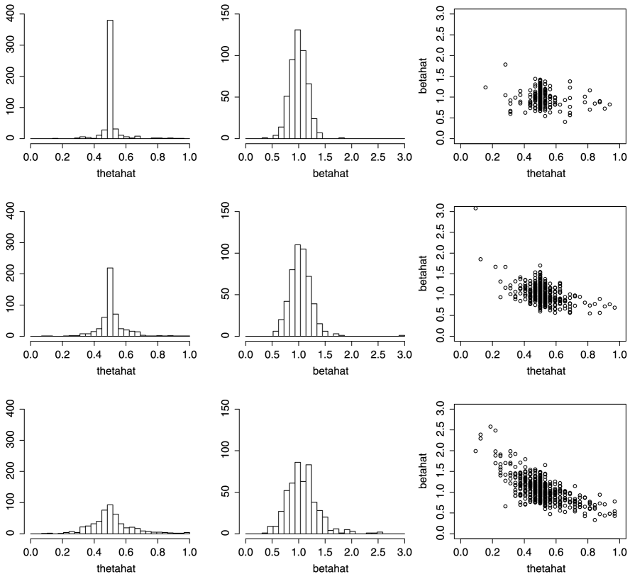
In practice, can only be observed at discrete time points, so restricting to a grid is the natural formulation for this example. Indeed, the resolution of the observation times in the neighborhood of is a limiting factor for the accuracy of , so the grid resolution needs to be fine enough for the statistical behavior of to be apparent. For large sample sizes, a very fine grid would be needed in the case of a small Hurst exponent (cf. Theorem 2.1). Indeed, the histogram of in the case (the first plot in Figure 2) shows that the resolution of the grid is almost too coarse to see the statistical variation, as the bin centered on contains almost 80% of the estimates. This phenomenon is also observed in Table 1 when and . The average length of the CIs is smaller than the resolution of the grid and, thus, we observe an over-coverage. The two histograms of for and , however, show increasing dispersion and become closer to bell-shaped as increases.
Recall that, for simplicity, we pretend as if we know , which should be an advantage, yet the residual bootstrap has better performance based on the results in Table 1. We see that usually the Wald-type CIs have coverage less than the nominal 95%, whereas the inconsistent nonparametric bootstrap method over-covers with observed coverage probability close to 1. Accordingly, the average lengths of the Wald-type CIs are the smallest, whereas those obtained from the nonparametric bootstrap method are the widest. The behavior of CIs obtained from the nonparametric bootstrap method also illustrates the inconsistency of this procedure. A similar phenomenon was also observed in LM06 in connection with estimators that converge at -rate.
Despite the asymptotic independence of and , considerable correlation is apparent in the scatterplots in Figure 2, with increasing negative correlation as increases; note, however, that when there is a lack of identifiability of and , so the trend in the correlation as approaches 1 is to be expected in small samples.
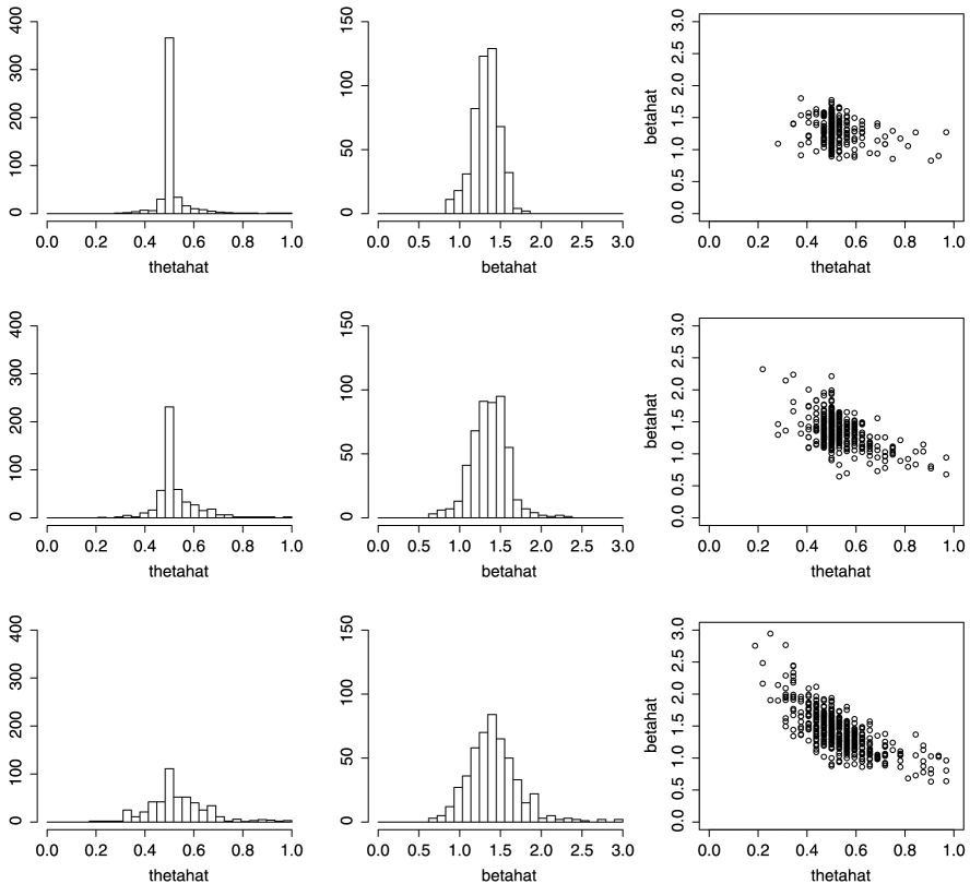
Next we consider a partially misspecified example, in which the data are now generated from (9) by setting and , but the other ingredients are unchanged from the correctly specified example. The plots in Figure 2 correspond to those in Figure 3. The effect of misspecification on is a slight increase in dispersion but no change in mean; the effect on is a substantial shift in mean along with a slight increase in dispersion.
6.1 Gene expression example
Next we consider the gene expression data mentioned in connection with Figure 1, to see how the residual bootstrap performs with such trajectories. The trajectories consist of log gene expression levels from the breast tissue of breast cancer patients, along a sequence of 518 loci from chromosome 17. The complete gene expression data set is described in Richardson et al. rich . Although a continuous response is not available for this particular data set, it is available in numerous other studies of this type; see the references mentioned in the Introduction.
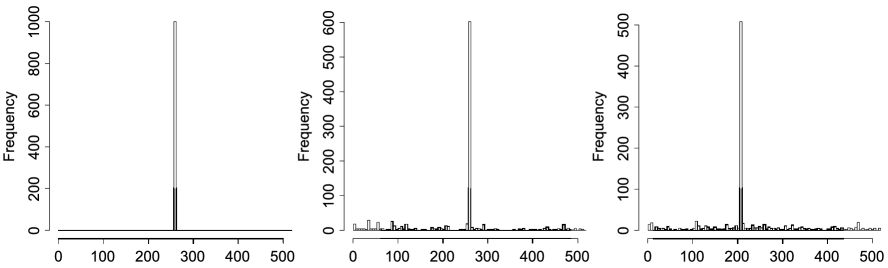
To construct a scalar response, we generated using the point impact model (1) with and , (corresponding to the position of 259 base pairs along the chromosome) and for various values of . As previously noted, the trajectories are very rough in this example (with estimated to be about 0.1), which implies a rapid rate of convergence for . We find that an abrupt transition in the behavior of the residual bootstrap occurs as increases: for small , the residual bootstrap estimates become degenerate at due to the relatively coarse resolution; for moderately large , although a considerable portion of the estimates are concentrated at , they become spread out over the 518 loci; for very large , the estimates are more or less uniformly scattered along the chromosome. Indeed, this is consistent with the behavior of the Wald-type CI (14) having width proportional to , which blows up dramatically as increases when is small.
In Figure 4 we plot the bootstrap distribution of (obtained from 1000 residual bootstrap samples in each case) for 0.01, 0.03 and 0.1. When , the bootstrap distribution is degenerate at ; the resolution of the grid is too course to see any statistical fluctuation in this case. When is moderate, namely, 0.03, although the bootstrap distribution has a peak at , the mass is widely scattered and the resulting CI now covers almost the entire chromosome. Further increasing the noise level causes the bootstrap distribution to become even more dispersed and its mode moves away from ; the sample size of 40 is now too small for the method to locate the neighborhood of .
7 Concluding remarks
In this paper we have developed a point impact functional linear regression model for use with trajectories as predictors of a continuous scalar response. It is expected that the proposed approach will be useful when there are sensitive time points at which the trajectory has an effect on the response. We have derived the rates of convergence and the explicit limiting distributions of the least squares estimator of such a parameter in terms of the Hurst exponent for fBm trajectories. We also established the validity of the residual bootstrap method for obtaining CIs for sensitive time points, avoiding the need to estimate the Hurst exponent. In addition, we have developed some results in the misspecified case in which the data are generated partially or completely from a standard functional linear model, and in the two-sample setting.
Although for simplicity of presentation we have assumed that the trajectories are fBm, it is clear from the proofs that it is only local properties of the trajectories in the neighborhood of the sensitive time point that drive the theory, and thus the validity of the confidence intervals. The consistency of the least squares estimator is of course needed, but this could be established under much weaker assumptions (namely, uniform convergence of the empirical criterion function and the existence of a well-separated minimum of the limiting criterion function; cf. vw , page 287).
Exploiting the fractal behavior of the trajectories plays a crucial role in developing confidence intervals based on the least squares estimator of the sensitive time point, in contrast to standard functional linear regression where it is customary to smooth the predictor trajectories prior to fitting the model (rs , Chapter 15). Our approach does not require any preprocessing of the trajectories involving a choice of smoothing parameters, nor any estimation of nuisance parameters (namely, the Hurst exponent). On the other hand, functional linear regression is designed with prediction in mind, rather than interpretability, so in a sense the two approaches are complimentary. The tendency of functional linear regression to over-smooth a point impact (see lmck for detailed discussion) is also due to the use of a roughness penalty on the regression function; the smoothing parameter is usually chosen by cross-validation, a criterion that optimizes for predictive performance.
Our model naturally extends to allow multiple sensitive time points, and any model selection procedure having the oracle property (such as the adaptive lasso) could be used to estimate the number of those sensitive time points. The bootstrap procedure for the (unregularized) least squares estimator can then be adapted to provide individual CIs around each time point, although developing theoretical justification would be challenging. Other challenging problems would be to develop bootstrap procedures that are suitable for the two-sample problem and for the misspecified model settings.
It should be feasible to carry through much of our program for certain types of diffusion processes driven by fBm, and also for processes having jumps. In the case of piecewise constant trajectories that have a single jump, the theory specializes to an existing type of change-point analysis kqs . Other possibilities include Lévy processes (which have stationary independent increments) and multi-parameter fBm. It should also be possible to develop versions of our results in the setting of censored survival data (e.g., Cox regression). Lindquist and McKeague lmck recently studied point impact generalized linear regression models in the case that is standard Brownian motion and we expect that our approach can be extended to such models as well.
8 Proofs
To avoid measurability problems and for simplicity of notation, we will always use outer expectation/probability, and denote them by and ; and will denote bootstrap conditional expectation/probability given the data.
We begin with the proof of Theorem 2.1. The strategy is to establish (a) consistency, (b) the rate of convergence, (c) the weak convergence of a suitably localized version of the criterion function, and (d) apply the argmax (or argmin) continuous mapping theorem.
8.1 Consistency
We start with some notation. Let and let , where denotes the expectation with respect to the empirical measure of the data. Let
First observe that has a unique minimizer at as , for all with .
Using the fBm covariance formula (4),
To show that is a consistent estimator of , first note that is uniformly tight. Also notice that is continuous and has a unique minimum at , and, thus, by Theorem 3.2.3(i) of vw , it is enough to show that uniformly on each compact subset of , and that has a well-separated minimum in the sense that for every open set that contains . That has a well-separated minimum can be seen from the form of the expression in (8.1). For the uniform convergence, we need to show that the class is -Glivenko Cantelli (-GC). Using GC preservation properties (see Corollary 9.27 of kbook ), it is enough to show that is -GC. Note that almost all trajectories of are Lipschitz of any order strictly less than , in the sense of (22) in Lemma 8.1 below. Thus, the bracketing number and is -GC, by Theorems 2.7.11 and 2.4.1 of vw .
8.2 Rate of convergence
We will apply a result of van der Vaart and Wellner (vw , Theorem 3.2.5) to obtain a lower bound on the rate of convergence of the M-estimator . Setting , the first step is to show that
| (17) |
in a neighborhood of . Here means that the right-hand side is bounded above by a (positive) constant times the left-hand side. Note that has a bounded derivative in , where is fixed, so for such we have
where is the bound on the derivative, , and we used the inequality . As and , by combining (8.1) and (8.2), suitably grouping terms, and noting that can be made arbitrarily small by restricting to a sufficiently small neighborhood of , there exist and such that
which shows that (17) holds.
Let , where . Note that
This shows that has envelope
Using a maximal inequality for fBm (Theorem 1.1 of nov ), we have
| (21) |
for any . Then, using (A3) in conjunction with Hölder’s inequality (cf. the proof of Lemma 8.1), all nine terms in (8.2) can be shown to have second moments bounded by (up to a constant) and, thus, .
The following lemma shows that is “Lipschitz in parameter” and, consequently, that the bracketing entropy integral is uniformly bounded as a function of ; see vw , page 294. Without loss of generality, to simplify notation, we assume that and , and state the lemma with as the only parameter.
Lemma 8.1
If (A1) and (A3) hold and , there is a random variable with finite second moment such that
| (22) |
for all almost surely.
The trajectories of fBm are Lipschitz of any order in the sense that
| (23) |
almost surely, where has moments of all orders; this is a consequence of the proof of Kolmogorov’s continuity theorem; see Theorem 2.2 of Revuz and Yor ry . Noting that , we then have
where and . Here has a finite second moment:
by Hölder’s inequality for with and comes from the moment condition (A3).
8.3 Localizing the criterion function
To simplify notation, let , for . Then
| (24) |
and we can write the expression in the square brackets after multiplication by as the sum of an empirical process and a drift term:
| (25) |
First consider the empirical process term, and note that
so we obtain
where (as a process in ).
The result of applying to the first term on the right-hand side of the above display gives a term of order uniformly in , for each . This is seen by applying the maximal inequality from vw , page 291, as used above; here the class of functions in question is bounded by the envelope function
for which and ; cf. the proof of Lemma 8.1. Hence, we just need to consider the second term. To determine the limit distribution of the empirical process term in (25), it thus suffices to show that
| (27) |
in , where are i.i.d. and independent of the fBm . For the second component above, notice that since is independent of ,
| (28) |
in . The asymptotic independence of the three components of (27) is a consequence of
which tends to zero uniformly in , using the assumption .
8.4 Proof of Theorem 3.1
We prove the result by the method of contradiction. Before giving the proof, we state a general lemma that can be useful in studying bootstrap validity. The lemma can be proved easily using characteristic functions; see also Sethuraman sethu and Theorem 2.2 of Kosorok k08 .
Lemma 8.2
Let and be random vectors in and , respectively; let and be distributions on the Borel sets of and , and let be -fields for which is -measurable. If converges in distribution to and the conditional distribution of given converges (in distribution) in probability to , then converges in distribution to .
The basic idea of the proof of the theorem now is to assume that in probability, where has the same distribution as . Therefore, unconditionally also. We already know that from Theorem 2.1. By Lemma 8.2 applied with , and , we can show that converges unconditionally to a product measure and, thus, . Thus, converges unconditionally to a tight limiting distribution which has twice the variance of .
Using arguments along the lines of those used in the proof of Theorem 2.1, we can show that
where is another independent fBm with Hurst exponent . Using properties of fBm, we see that
Thus, the variance of the limiting distribution of is times the variance of , which is a contradiction.
8.5 Proof of Theorem 3.2
The bootstrap sample is , where the are defined in (7). Letting , the bootstrap estimates are
| (29) |
We omit the rate of convergence part of the proof, and concentrate on establishing the limit distribution. Also, to keep the argument simple, we will assume that a.s., but a subsequence argument can be used to bypass this assumption. Note that
| (30) |
where is the probability measure generating the bootstrap sample. Consider the first term within the curly brackets. Using a similar calculation as in (8.3),
| (31) |
where , with the dependence on suppressed for notational convenience, and uniformly in . Then, using (31),
| (32) | |||
in , a.s., where are i.i.d. that are independent of .
To prove (8.5), first note that , as the are fixed and the have mean zero under . We will need the following properties of , proved at the end:
uniformly for , where is the covariance function (4) of fBm. Now considering (8.5), by simple application of the Lindeberg–Feller theorem, it follows that
a.s. in . Next consider . The finite-dimensional convergence and tightness of this process follow from Theorems 1.5.4 and 1.5.7 in vw using the properties of stated in (8.5). The asymptotic independence of the terms under consideration also follows using (8.5) via a similar calculation as in (29).
To study the drift term in (30), note that
Simple algebra then simplifies the drift term to
| (35) | |||
uniformly on , where we have used the properties of in (8.5) and
Thus, combining (30), (8.5) and (8.5), we get in probability.
It remains to prove (8.5). We only prove the last part, the other parts being similar. For fixed , consider the function class
which has a uniformly bounded bracketing entropy integral, and envelope
from the Lipschitz property (23) of order , where and has finite moments of all orders. Then
where we use a maximal inequality in Theorem 2.14.2 of vw .
Remark
The failure of the nonparametric bootstrap can be explained from the behavior of the drift term in (30). In the nonparametric bootstrap, we need to find the conditional limit of given the data, but observe that applied to the second term of (8.3) fails to converge in probability. However, when bootstrapping residuals, the drift term in (30) becomes , and applied to the second term in (8.3) vanishes, so the drift term now converges in probability, as seen in (8.5).
8.6 Proof of Theorem 4.1
The consistency of follows using a Glivenko–Cantelli argument for the function class and the existence of a well-separated minimum for ; cf. the proof of Theorem 2.1. Note that is the unique solution of the normal equation and , so
| (36) |
for all in a neighborhood of , where is the usual Euclidean distance. The envelope function for has -norm of order , from (21), so Theorem 3.2.5 of vw applied with gives rate with respect to Euclidean distance.
Now write , where
| (37) |
This gives
| (38) |
where uniformly in , for any , and
Note that as processes, so, by Donsker’s theorem, the first term in (38) converges to zero in probability uniformly over . For the second term, we claim that
| (39) |
as processes in , where . Application of the argmin continuous mapping theorem will then complete the proof.
To prove (39), for simplicity, we just give the detailed argument in the Brownian motion case, with denoting two-sided Brownian motion. Consider the decomposition
| (40) |
where
| (41) |
, and is sufficiently small so that . Splitting the range of integration for the first term in into three intervals, and using the integration by parts formula (for semimartingales) over the intervals and , we get
which implies, by the independent increments property, that is independent of for . Using the same argument as in proving (28), it follows that
as processes in , for each fixed , where
as . Clearly, in as . If we show that the last term in (40) is asymptotically negligible in the sense that, for every and ,
| (42) |
this will complete the proof in view of Theorem 4.2 in bill . Theorem 2.14.2 in vw gives
where is the bracketing entropy integral of the class of functions , and is an envelope function for . We can take . By the Cauchy–Schwarz inequality,
where we have used (21). The bracketing entropy integral can be shown to be uniformly bounded (over all and ) using the Lipschitz property (23). The previous two displays and Markov’s inequality then lead to
To establish (39) for general fBm, we apply Theorem 2.11.23 of vw to the class of measurable functions , where and is fixed. Direct computation using the covariance of fBm shows that the sequence of covariance functions of converges pointwise to the covariance function of , and the various other conditions can be shown to be satisfied using similar arguments to what we have seen already.
8.7 Proof of (13)
The key step involving the localization of the criterion function again relies on the self-similarity of fBm :
where is the empirical process for the th sample.
Acknowledgments
The authors thank Moulinath Banerjee and Davar Khoshnevisan for helpful discussions.
References
- (1) Beran, J. (1994). Statistics for Long-Memory Processes. Chapman and Hall, New York. \MR1304490
- (2) Bhattacharya, P. K. and Brockwell, P. J. (1976). The minimum of an additive process with applications to signal to signal estimation and storage theory. Z. Wahrsch. Verw. Gebiete 37 51–75. \MR0426166
- (3) Bickel, P. and Freedman, D. (1981). Some asymptotic theory for the bootstrap. Ann. Statist. 9 1196–1217. \MR0630103
- (4) Billingsley, P. (1999). Convergence of Probability Measures, 2nd ed. Wiley, New York. \MR1700749
- (5) Buness, A. et al. (2007). Identification of aberrant chromosomal regions from gene expression microarray studies applied to human breast cancer. Bioinformatics 23 2273–2280.
- (6) Chernoff, H. (1964). Estimation of the mode. Ann. Inst. Statist. Math. 16 31–41. \MR0172382
- (7) Coeurjolly, J.-F. (2008). Hurst exponent estimation of locally self-similar Gaussian processes using sample quantiles. Ann. Statist. 36 1404–1434. \MR2418662
- (8) Dudoit, S. and van der Laan, M. J. (2008). Multiple Testing Procedures with Applications to Genomics. Springer, New York.
- (9) Embrechts, P. and Maejima, M. (2002). Selfsimilar Processes. Princeton Univ. Press, Princeton. \MR1920153
- (10) Emilsson, V. et al. (2008). Genetics of gene expression and its effect on disease. Nature 452 423–428.
- (11) Gneiting, T. and Schlather, M. (2004). Stochastic models that separate fractal dimension and the Hurst effect. SIAM Rev. 46 269–282. \MR2114455
- (12) Groeneboom, P. and Wellner, J. A. (2001). Computing Chernoff’s distribution. J. Comput. Graph. Statist. 10 388–400. \MR1939706
- (13) Gruvberger-Saal, S. K. et al. (2004). Predicting continuous values of prognostic markers in breast cancer from microarray gene expression profiles. Molecular Cancer Therapeutics 3 161–168.
- (14) Härdle, W. and Mammen, E. (1993). Comparing nonparametric versus parametric regression fits. Ann. Statist. 21 1926–1947. \MR1245774
- (15) Kim, J. and Pollard, D. (1990). Cube root asymptotics. Ann. Statist. 18 191–219. \MR1041391
- (16) Kosorok, M. (2008). Bootstrapping the Grenander estimator. In Beyond Parametrics in Interdisciplinary Research: Festschrift in Honour of Professor Pranab K. Sen (N. Balakrishnan, E. Pena and M. Silvapulle, eds.) 282–292. IMS, Beachwood, OH. \MR2464195
- (17) Kosorok, M. (2008). Introduction to Empirical Processes and Semiparametric Inference. Springer, New York.
- (18) Koul, H. L., Qian, L. and Surgailis, D. (2003). Asymptotics of M-estimators in two-phase linear regression models. Stochastic Process. Appl. 103 123–154. \MR1947962
- (19) Lieberman-Aiden, E., van Berkum, N. L., Williams, L. et al. (2009). Comprehensive mapping of long-range interactions reveals folding principles of the human genome. Science 326 289–293.
- (20) Léger, C. and MacGibbon, B. (2006). On the bootstrap in cube root asymptotics. Canad. J. Statist. 34 29–44. \MR2267708
- (21) Lindquist, M. A. and McKeague, I. W. (2009). Logistic regression with Brownian-like predictors. J. Amer. Statist. Assoc. 104 1575–1585.
- (22) Mandelbrot, B. B. and Van Ness, J. (1968). Fractional Brownian motions, fractional noises and applications. SIAM Rev. 10 422–437. \MR0242239
- (23) Mandelbrot, B. B. (1982). The Fractal Geometry of Nature. Freeman, New York. \MR0665254
- (24) Müller, H.-G. and Song, K.-S. (1997). Two-stage change-point estimators in smooth regression models. Statist. Probab. Lett. 34 323–335. \MR1467437
- (25) Neumeyer, N. (2009). Smooth residual bootstrap for empirical processes of non-parametric regression residuals. Scand. J. Statist. 36 204–228. \MR2528982
- (26) Novikov, A. and Valkeila, E. (1999). On some maximal inequalities for fractional Brownian motions. Statist. Probab. Lett. 44 47–54. \MR1706311
- (27) Ramsay, J. O. and Silverman, B. W. (2006). Functional Data Analysis, 2nd ed. Springer, New York. \MR2168993
- (28) Revuz, D. and Yor, M. (1999). Continuous Martingales and Brownian Motion, 3rd ed. Springer, New York.
- (29) Richardson, A. L., Wang, Z. C., De Nicolo, A., Lu, X. et al. (2006). chromosomal abnormalities in basal-like human breast cancer. Cancer Cell 9 121–132.
- (30) Salas-Gonzalez, D., Kuruoglu, E. E. and Ruiz, D. P. (2009). Modelling and assessing differential gene expression using the alpha stable distribution. Int. J. Biostat. 5 23. \MR2504963
- (31) Sethuraman, J. (1961). Some limit theorems for joint distributions. Sankhyā Ser. A 23 379–386. \MR0139190
- (32) Shao, J. and Tu, D. (1995). The Jackknife and Bootstrap. Springer, New York. \MR1351010
- (33) Singh, K. (1981). On asymptotic accuracy of Efron’s bootstrap. Ann. Statist. 9 1187–1195. \MR0630102
- (34) Stryhn, H. (1996). The location of the maximum of asymmetric two-sided Brownian motion with triangular drift. Statist. Probab. Lett. 29 279–284. \MR1411427
- (35) van der Vaart, A. and Wellner, J. A. (1996). Weak Convergence and Empirical Processes. Springer, New York. \MR1385671
- (36) Van Keilegom, I., González-Manteiga, W. and Sánchez Sellero, C. (2008). Goodness-of-fit tests in parametric regression based on the estimation of the error distribution. Test 17 401–415. \MR2434335
- (37) Yao, Y.-C. (1987). Approximating the distribution of the maximum likelihood estimate of the change-point in a sequence of independent random variables. Ann. Statist. 15 1321–1328. \MR0902262