Fractional Lotka-Volterra model with time-delay and delayed controller for a bioreactor
Abstract
In this paper, a fractional Lotka-Volterra mathematical model for a bioreactor is proposed and used to fit the data provided by a bioprocess known as continuous fermentation of Zymomonas mobilis. The model contemplates a time-delay due to the dead-time in obtaining the measurement of biomass . A Hopf bifurcation analysis is performed to characterize the inherent self oscillatory experimental bioprocess response. As consequence, stability conditions for the equilibrium point together with conditions for limit cycles using the delay as bifurcation parameter are obtained. Under the assumptions that the use of observers, estimators or extra laboratory measurements are avoided to prevent the rise of computational or monetary costs, for the purpose of control, we will only consider the measurement of the biomass. A simple controller that can be employed is the proportional action controller , which is shown to fail to stabilize the obtained model under the proposed analysis. Another suitable choice is the use of a delayed controller which successfully stabilizes the model even when it is unstable. Finally, the proposed theoretical results are corroborated through numerical simulations.
Keywords: bioreactor, bifurcations, time-delay systems, fractional mathematical model.
1 Introduction
In addition of its academic and performance predictive importance, mathematical models for bioreactors are required tools for implementing process control strategies demanded in industrial bioprocess. Using these devices, researches have successfully cultivated important kind of cells for the pharmaceutic industry [13], developed complex organ cultures [8, 32], designed wastewater treatments [2, 29], increased hydrogen production [18], and studied microbial biomass and energy conversion [15], among many other relevant applications.
In the case of culturable microbial species, the literature contains numerous examples modeling their iteration [19, 44, 46] and their consequent production of biochemical substances [28]. A fundamental part of bioprocessing is to create favorable environmental conditions for microorganisms based on different substrate compositions. In order to achieve this conditions, positive feedback loops are essential. Mathematically speaking, this amounts to the need to have parametric conditions for the characterization of bifurcations and the appearance of limit cycles of the dynamical system modeling the bioreactor. In the literature, modeling and bifurcation analysis using the dilution rate as a parameter are predominant.
It is known that laboratory observations exhibit oscillatory behavior. The oscillatory behavior manifests itself as the self-sustained oscillations (SSO) among key process variables and parameters (e.g. substrate, biomass, metabolites, dilution rate, temperature, agitation speed, pH, constant feed and culture conditions) [50, 49]. Consequently, diverse phenomena, such as multiplicity of steady states, stability of limit cycles or chaoticity, may be present in the bioprocess [47, 48, 51]. In some bioprocesses it has been observed that the oscillatory mode of operation can have higher performance in comparison to the obtained in steady-state regime (e.g. higher biomass and metabolites concentrations) [9, 17, 53]. Therefore it as important to understand the conditions for the oscillatory process and as it is highly desirable to know how to attenuate the oscillatory changes in the product concentration (biomass and metabolites). The above can be resolved via the manipulation of a parameter (set point: dilution rate, temperature, pH or dissolved oxygen), the use of input effluent stabilization tanks, or by the design of controllers that stabilize self-oscillating bioreactors by manipulating the input [16].
Naturally, delays are always present in bioprocesses, since there are dead times between biological reactions/interactions, metabolization of substances, considerations of past population rates, among others. Therefore, it is necessary to consider these in mathematical modeling [10, 25, 31, 39, 41, 43].
Some members of the scientific community have argued that time delays should be omitted or disregarded from mathematical models since they may cause undesirable/poor behavior in the system response or even compromise its stability. However, this interpretation is wrong. In the last two decades a part of the scientific community has devoted efforts to studying the effect of considering time-delays, dead-time or just delays in mathematical models [1, 6, 33, 34, 35, 38, 40, 42]. As previously mentioned, the delays are inherent (perceptible or not with the naked eye) in the real/experimental processes so that the omission of these in the mathematical models seems to be only for the purpose of facilitating its analysis.
Although the analysis of a mathematical model is rather harder for dynamical systems admitting a delay, this paper attempts to provide one more example that this extra work is worthwhile as the use of a delay allows the fitting of data from a real/experimental process. For example, delays seen as bifurcation parameters are useful tools in obtaining conditions for the existence of limit cycles and Hopf bifurcations. Furthermore, delays may create the conditions for the stabilization of a system otherwise unstable. In the last decade it has been shown that the deliberate inclusion of delays in the control laws can substitute the development of observers/estimators of unavailable state variables [14, 24, 26]. In addition to reducing the noise present in measuring instruments [21]. In bioprocesses, costs can be reduced by avoiding biomass or substrate measurement tests.
In this work a fractional Lotka-Volterra model with time delay and delayed controller for a bioreactor, which will turn out to fit the data provided by a bioprocess known as continuous fermentation of Zymomonas mobilis, is proposed. Afterwards a mathematical analysis is conducted providing conditions for the appearance of a Hopf bifurcations and stability of a equilibrium point using the delay as a bifurcation parameter. The novelty of our approach relays on three facts. The first one is that the proposed mathematical model uses fractional exponents to scale the state variables, an approach successfully used to model the dynamics of cancer cell [37] and in epidemiology models [36]. Secondly is the inclusion of a time-delay and thirdly the inclusion of a delayed controller to manipulate the inflow of the substrate to stabilize the bioreactor model even under unstable conditions. This approach allows the design and tuning of delayed control laws to minimize costs and maximize productions of bioprocessing. To illustrate the theoretical results proposed here, we present numerical simulations.
The paper is organized as follows. The description of the biological system is shown in Section 2. A description of the proposed fractional Lotka-Volterra model with time-delay and delayed controller together with the corresponding mathematical analysis are presented in Section 3. Here, we use to identify the parameters of the model and to characterize the critical parameters of which allow limit cycles and Hopf bifurcations. Then, we propose for the design and tuning of a delayed controlled to -stabilize the model. In Section 4, the implementation and validation of the previous theoretical results are given. Concluding remarks are stated in Section 5. Finally, some notation and preliminary results concerning to stability of time-delay system are stated in the Appendix.
2 Description of the bioreactor
In this section we present the description of the physical plant. It was the desire of modeling and controlling such a plant that motivated the present work. Although these bioprocess are well understood, we were unable to find in the literature a specific mathematical model fitting the data obtained in our experiments.
In Figure 1 we present a diagram showing a pair of tanks composing the basic structure of our bioreactor. The main tank, where the mixing occurs, is where the inoculum lies. We then supply a percentage of the substrate to enter this tank through a valve from the secondary tank.

The fermentation in continuous operation were carried out in a bioreactor containing broth medium 50 ml in a volume of 250 ml, inoculated with colonies of Zymomonas mobilis for 80 hours. Samples were incubated at C and 100 rpm. This experiment was performed in triplicate. Cocoa juice was extracted from cocoa fermentation baskets after two days. Juice samples were immediately stored in sterile bottles. For experiments, cocoa pulp juice was adjusted to 10 g/L of glucose with reducing sugar. Reaction mixture was analyzed by the reducing sugar, applying the 3,5-dinitrosalicyclic acid method [20]. The quantity of reducing sugars was calculated using the regression equation, consisting of a standard curve with glucose (1 mg/mL). The bacterial biomass growth was evaluated by dry weight method [3]. A 5 mL-aliquot was taken 5 hours for analyses of biomass and substrate.
Next, a description of the experiment when the maximum biomass an minimal substrate is obtained. Substrate consumption of cocoa bean pulp during fermentation occurred during the first 25 h of fermentation until a remnant of 0.9 g/L remained. Changes in glucose concentration demonstrated metabolic changes during the fermentation of different hybrids. A decrease in substrate favored the growth of biomass because these microorganisms use this chemical compound as substrate [22]. The maximum biomass concentration in the treatment of glucose to 8.1 g /L was obtained in the first 20 h of a operation in continuous fermentation for a dilution rate of 0.15 1/h. The experimental data obtained in the bioprocess is given in Table 1. Note that an oscillatory behaviour is observed in the dynamics of the experimental bioprocess.
| Time | Biomass | Error | Substrate | Error |
|---|---|---|---|---|
| 0 | 0.1 | 0.005 | 10.0 | 0.5 |
| 5 | 0.3 | 0.015 | 9.0 | 0.45 |
| 10 | 1.1 | 0.055 | 7.8 | 0.4 |
| 15 | 4.3 | 0.215 | 6.1 | 0.33 |
| 20 | 8.1 | 0.405 | 3.4 | 0.175 |
| 25 | 5.1 | 0.255 | 0.9 | 0.045 |
| 30 | 4.0 | 0.20 | 2.1 | 0.105 |
| 35 | 4.5 | 0.225 | 2.6 | 0.13 |
| 40 | 5.1 | 0.255 | 1.6 | 0.08 |
| 45 | 4.9 | 0.245 | 1.9 | 0.095 |
| 50 | 4.3 | 0.215 | 2.5 | 0.125 |
| 55 | 4.9 | 0.245 | 1.7 | 0.085 |
| 60 | 4.1 | 0.205 | 2.4 | 0.12 |
| 65 | 5.0 | 0.25 | 1.6 | 0.08 |
| 70 | 4.2 | 0.21 | 2.3 | 0.115 |
| 75 | 4.9 | 0.245 | 1.4 | 0.07 |
| 80 | 4.0 | 0.20 | 2.0 | 0.1 |
3 Description and analysis of mathematical model
This section presents a description and mathematical analysis of the fractional Lotka-Volterra model with time-delay and delayed controller. First, the model is presented together with a theoretical justification. Next, the analysis of the model with constant excitement is conducted and finally an analysis of the model with the delayed controller, including a description for the tuning of the controller is included. It is important to emphasize that, in the next section, our model will be shown to fit the experimental data described in the previous section.
3.1 Description of the fractional Lotka-Volterra model with time delay for a bioreactor
In this subsection a fractional Lotka-Volterra model with time-dealy for a bioreactor based on the Lotka–Volterra equations is introduced. One reason for choosing this well known predator-prey mathematical model is the appearance of periodic solutions, a phenomena observed in the experimental data of a bioreactor. Evidently, the Lotka-Volterra equations alone are not able to capture the rich variety of dynamics involved in a bioreactor. For this purpose, two context specific modifications are proposed: By following an approach gaining prominence in dealing with these complexities, first fractional exponents in the variables have been introduced [36, 37], and secondly, a time-delay term has been added in one of the differential equations [7]. In doing so it turned out the the mathematical model adequately fits the data provided.
For modeling a bioreactor, the following fractional Lotka-Volterra equations with time-delay and delayed control is introduced:
| (1) |
where are constant positive parameters of the bioreactor, are positive fractional-exponents, is the positive initial supply of substrate, is a non-negative constant delay, is the amount of substrate present in the bioreactor at time , is the amount of such produced biomass at time , and is the input signal to manipulate the inflow of substrate into the bioreactor.
When setting , the first equation in the model (1) reduces to . That is to say, in the absence of biomass, the rate of change of the substrate is proportional to a scaling of the substrate by an exponent . The negative sign reflects that the substrate in the bioreactor actually decays in the absence of biomass, in contrast to a classical Lotka-Volterra approach where intrinsic rate of prey population increase. It has been observed experimentally that the value of satisfy the inequality , in particular the substrat, in absence of biomass, is subject to a non-exponential decay.
On the other hand, for , the second equation in the model (1) becomes . That is to say, in the absence of substrate, the biomass follows a decay proposed in the Norton-Simons-Massagué (NSM) model. While the the NSM model actually describes the growth of tumors, the sign of the terms on the right hand side of the NSM model have been reversed to describe instead the decay of an organism under energy constrains. This approach has been successfully taken in very recent works on the analysis of cancer cells [37] and epidemiological models [36]. Here lies another of the proposed modification of the classical Lotka-Volterra model, where the rate of change of predators in absence of prey is assumed to be proportional to their population.
The Lotka-Volterra equations are complemented with the terms containing the scaled products which represent the rates of decay and growth provided by the biochemical iterations between substrate and biomass. That is to say, the terms and replace and used in the original model, respectively. The populations and are considered to be scaled by the same exponents and described above.
Finally, the delay in the variable in the first equation of the system (1) is justified as follows: the effect of the biomass in the rate of consumption of the substrate is affected by a dead time produced either by a gestation time-delay or by a time delayed measurement. Mathematically, this delay will turn out to produce the possibility for a stable equilibrium point of the fractional Lotka-Volterra model (1), in sharp contrast with the non-stability of equilibrium points of a classical Lotka-Volterra model. Thus the introduction of this time-delay favors the modeling of our bioreactor, where stability of fixed points is observed experimentally. Furthermore, biomass production can only be manipulated indirectly by supplying substrate , so that the only controllable variable is the substrate through a control action that regulates the flow of the substrate through the bioreactor. Here represents zero flow (valve fully closed) and represents total flow (valve fully open), see Figure 1. Therefore, the first equation in (1) has control action while the second equation has no control action.
A summary of the parameters in the fractional Lotka-Volterra model (1) is shown next.
-
•
The parameter is the intrinsic rate of the amount of scaled substrate [Units: 1/h].
-
•
The parameter is the fractional-exponent scaling the amount of substrate [Units: Dimensionless].
-
•
The parameter is the rate of consumption of the scaled substrate by the scaled biomass [Units: 1/h].
-
•
The parameter is the fractional-exponent of growth of the biomass [Units: Dimensionless].
-
•
The parameter denotes the net rate of growth the scaled biomass in response to the size of the scaled substrate [Units: 1/h].
-
•
The parameter measures the output of the scaled biomass from the bioreactor [Units: 1/h].
-
•
The parameter quantifies anabolism (growth rate) of the biomass.
3.2 Analysis of mathematical model with constant excitement
To obtain a parametric identification of the model proposed in (1), we begin by assuming that the input signal is constant and positive. This amounts to open the valve for the substrate to a constant input flow. Our purpose is to achieve the tuning of the parameters so that our model resembles the experimental data of a bioreactor. In addition, we will give conditions for obtaining limit cycles and Hopf bifurcations using the time-delay as a bifurcation parameter.
Thus, the mathematical model (1) is rewritten as
| (2) |
Proposition 1.
Suppose that the equation
| (3) |
has a root such that . Denote
Then is a positive equilibrium point of the model given in (2).
Proof.
Let us assume that and denote the equilibrium point of (2), in particular, and . Whence, the second equation of (2) becomes
or equivalently
Solving for in the last equation above we obtain
On the other hand, by substituting the above expression for in the first equation of (2) we get
Hence, by solving the following equation for
we obtain the desired equilibrium point. ∎
We remark that in our setting, equation (3) does admit a positive solution such that . For completeness of our analysis, next we provide some algebraic conditions for such solution to exist, namely, conditions for the left hand side of equation (3) to change of sign for a couple of values of . Indeed, if then and so the left hand side of equation (3) reduces to which is positive. Similarly if then and so the left hand side of equation (3) reduces to . Thus, a condition for the left hand side of equation (3) to be negative and hence for equation (3) to admit a nonzero solution is . In in addition one requires the inequality one also guarantees that . In what follows, we will assume that the equilibrium points and obtained from Proposition 1 are both positive.
Using Proposition 1, the linearization of system (2) is of the form (23), where
, and its quasi-polynomial is
| (4) |
with
The stability of system (2) is completely determined by the location of the roots of its corresponding characteristic quasi-polynomial (4). D-partition method proposed by Neimark in [23] determine stability conditions of a quasi-polynomial through study of the space of crossover frequencies -crossing delays. Below, we employ this method to the quasi-polynomial (4). In addition, we will assume the the system is initially stable, that is, stable when .
A stable quasi-polynomial loses stability if some of its roots cross to the open right-half of the complex plane. Clearly, the above occurs when the roots first cross the imaginary axis. For this, there are two possible cases: i) purely imaginary crossover window , where , ii) crossover window on the origin . In both cases, must be solution of quasi-polynomial. In general, the crossover window occur under variations of the parameters of a system or quasi-polynomial. A particular case and of great interest to the scientific community since it is closely related to bifurcation theory, it is to find the crossover windows when delay varies. Next, an analysis of the quasi-polynomial (4) using the mentioned above is performed.
Consider the change of variable in the quasi-polynomial (4)
Clearly, we cannot obtain stability conditions from the previous equation whence, efforts will be focused when , , is solution of quasi-polynomial (4),
Note that, iff
For the above, we have
Therefore, the following is satisfied
| (5) |
Thus, the quasi-polynomial (4) has roots , if is solution of the polynomial given in (5). Moreover, the delay value where the above occurs is
| (6) |
Next, we postulate in the following criteria the stipulated above.
Proposition 2.
The previous result provides conditions of the delay for which the quasi-polynomial (4) has roots on the imaginary axis . If these roots are dominant, then it is natural to determine when the roots move to the right half-plane under infinitesimal variations of this delay . The above is know as direction of the crossing [45] and it is determined using the following result.
Proposition 3.
Proof.
The technique will need to check for each root on the imaginary axis crosses to the left or to the right of the complex plane when increasing . This is determined by the sign of . Consider the quasi-polynomial given in (4) and suppose that , then
which implies that
Therefore, for yields
Thus, for we get
This ends the proof. ∎
Note that the sign given in (7) is independent of , therefore if the linearization of system (2) is stable for , then it remains stable for all , where is the first value of (6). Thus the following result is evident.
Proposition 4.
3.3 Analysis of mathematical model with delayed controller
In this section, we carry out a stability analysis of the fractional mathematical model (1) in closed-loop with a delayed controller of the type (24). As well as tuning the controller gains.
Proposition 5.
Let be a positive real number such that
If
then and are the equilibrium point of the fractional mathematical model (1).
Proof.
Let us assume that , and denote the equilibrium point of the model (1). Then the second equation of (1) becomes
and solving for we obtain
Now, the first equation of (1) we obtain
The hypothesis imply that . Thus for the fixed positive value , and the value of satisfying the given inequalities, the value of is obtained so that they are equilibrium point, as was to be shown. ∎
Using Proposition 5, the linearization of model (1) is of the form (23), where
| (8) |
Next, we propose the following delayed controller to stabilize the model
| (9) |
where is the controller gain and is the controller delay. Note that in (9) the proposed controller is only acting on the biomass and not on the substrate . We base our proposal in the fact that, during the experiments, we only have access to the measurement of and not of . In addition, the time-delay in the controller is justified by the time-delay in between the recordings of the biomass output.
Let and given in (8), then the quasi-polynomial of closed-loop systems (23) with (9) is
| (10) |
where
| (11) |
3.3.1 Tuning of the delayed controller
Here again we use the D-partition method proposed by Neimark [23] and the tuning method proposed in [42]. Consider the quasi-polynomial given in (3.3) and the chance of variable , for a given , i.e.
| (12) | ||||
If note that the above quasi-polynomial is
therefore
If note that the quasi-polynomial (12) is
the previous equality is satisfied if
| (13) | ||||
| (14) |
where
| (15) |
Solving for of (14) we obtain
By substituting the above equation in (13) we get
Solving of above equation
Next, we postulate a result for tuning the delayed controller (9) using the above.
4 Validation of theoretical results
4.1 Validation of mathematical model
As mentioned before, for parametric identification, in this section we assume that in the mathematical model (1). In addition, experimental data is taken from a biochemical process as reference points to identification, see Table 1. For the simulations, we consider initial conditions of g/L for the substrate and g/L for the biomass, as well as a constant opening of the substrate flow valve equal 1/h. These initial parameters are the same as those implemented in the biochemical process described above. To obtain the values of the other parameters nonlinear regression was used based on the Levenberg-Marquardt least squares minimization algorithm. In consequence, the values obtained from our model come closer to the experimental data, see Figure 2 and 3. They are
| (16) |
Whereby, , and . The parameter values obtained in the present study fall within the range of those reported in the literature, due to the different operating conditions used in each case, i.e., different carbon source, continuous or batch operation, temperature, pH, among others ([4, 27, 30, 52]).

The performance of the proposed mathematical model was statistically validated using the dimensionless coefficient of efficiency , where
, is the simulated value of the variable at time , is the observed value of the same variable at time and the mean value of the observed variable. A positive value of represents an acceptable simulation, whereas represents good simulation [5, 12].
It is recommended, therefore, to use () in lieu of correlation-based measures to provide a relative assessment of model performance. The statistics used absolute values rather than squared differences. Parameter efficiency () for all variables using the L-M method are: Biomass (0.850) and Substrate (0.834) and, Interpretation of correlation-based measures, 0.85 indicate that the model explains 85.0% of the variability in the observed data. Therefore, the proposed model was able to predict experimental data.
Now, using Proposition 1 and parameters given in (16) an equilibrium point of the mathematical model (2) is
| (17) |
Therefore, the linearization of (2) using (16) and (17) is
and by (4) its quasi-polynomial is
Thus, the polynomial (5) gives
Finally, using Proposition 5 and the solution of the above polynomial, we get some candidate values of delay which may be critical values of , where the mathematical model (2) has a Hopf bifurcation. Some calculated critical values are
| (18) |
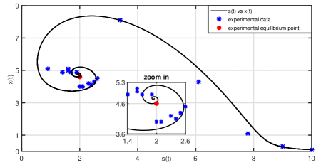
These values were obtained using the equation (6) for . To corroborate that the points given in (18) are critical points, in Figure 4 the phase diagrams of model (2) are presented. Note that for initial conditions near the equilibrium point (17), even more the system response (2) remains oscillating around the equilibrium point, thus verifying the existence of a limit cycle on .

While in Figure 5 the stability of the model (2) for is shown, using phase diagrams. Note that for the same initial condition , but different values of , the system response converges to the equilibrium point (17), corroborating the stability of (2) for all , as postulated in the Proposition 4.

On the other hand, by Proposition 3 we have that (7) is
Thus, in Figure 6, the system response and a phase diagram of (2) are presented, when . Clearly, the solution diverges from the equilibrium point (17), showing via simulation that the model (2) is unstable, when and the initial condition is nearby the equilibrium point and corroborating the provisions of the Proposition 4.

4.2 Implementation of delayed controller
Consider the parameters given in (16), . By Proposition 5 and given, the equilibrium point of the model (1) is
| (19) |
Thus, the linearization of (1) using (8) is
| (20) |
and the quasi-polynomial (3.3) is
| (21) |
Using Proposition 6, the -stability regions in the parametric plane are given in Figure 7 for . Notice that these regions are concentric and their size decreases as increases. Furthermore, a collapse of these regions to the point marked with a red asterisk can be observed when , which implies that is the maximum achievable exponential decay of the linear systems (20) or quasi-polynomial (21).
The following observations may be proposed:
- •
- •
- •
- •
- •

To ratify the above, Figure 8 shows the response of the mathematical model (1) when and . Here, the initial condition is and the applied control is for , once the instability of the model (1) can be observed, then the control is applied. In other words, consider the model given in (1), the initial condition , the parameters (16) and , the mathematical model response (1) is depicted in Figure 8, when
where , , , and the gains and of the delayed controller are only the four points , , marked with in Figure 7, namely , , and . Corresponding to border points of the -stable regions, when and . Furthermore, as mentioned in Definitions 1 and 2, this determines the exponential decay in the system response (1), which can also be observed in Figure 8. The signals delayed controller (9) with , applied to the mathematical model (1) as depicted in Figure 9. It is clear that this control signal is within the range established for and this signal exponentially stabilize model fractional mathematical model (1), even though it is initially unstable for . Calculation of the distribution of Hopf point contributed to enhancing the stability of the fermentation process, maintaining high product quality, and providing insights into system dynamics.


5 Conclusions
In this article a fractional Lotka-Volterra mathematical model with time-delay is presented fitting the data provided by a biochemical process in a bioreactor known as Zymomonas mobilis. This model allows an analysis to determine Hopf bifurcations when the delay is used as a bifurcation parameter. Furthermore, a well-founded proposal for the design and tuning of delayed controllers to stabilize the biochemical process is given. The efficiency and effectiveness of the theoretical results formulated are illustrated by numerical simulation. It is worth pointing out those bifurcations regions of operation and control of oscillatory dynamics in the biosystem are of practical importance as they possess many potential applications in biofuels, medical science and biochemistry. This is due to the fact that these systems have a time delay in common in their signals as consequences of dead time in the quantification of a state.
Appendix: Time-delay systems
Since we consider delays in the mathematical model used to describe the dynamics of the biorector, some concepts and criteria on the stability of time-delay systems are postulated in this Appendix.
Consider a time-delay nonlinear system of the form
| (22) |
where , , and = . For denote by the solution of the system with initial condition , and by the Banach space with norm . Finally, denotes the euclidean norm.
The equilibrium , is the one that satisfies Thus, the linearization of (22) at the equilibrium point is
| (23) |
where
,
with ,
and
, , .
Now, consider a delayed controller of the form
| (24) |
where and is a delay (equal or different from ). If , then the closed-loop (23)-(24) is
| (25) |
Thus, the characteristic equation (quasi-polynomial) of system (25) is of the form
| (26) |
Definition 1.
References
- [1] C. Abdallah, P. Dorato, J. Benites-Read, and R. Byrne. Delayed positive feedback can stabilize oscillatory systems. In American Control Conference, 1993, pages 3106–3107. IEEE, 1993.
- [2] L. Appels, J. Baeyens, J. Degreve, and R. Dewil. Principles and potential of the anaerobic digestion of waste-activated sludge. Progress in Energy and Combustion Science, 34(6):755–781, 2008.
- [3] American Public Health Association, American Water Works Association, Water Pollution Control Federation, and Water Environment Federation. Standard methods for the examination of water and wastewater. American Public Health Association, Washington DC, 14th edition, 1976.
- [4] E.A. Buehler and A. Mesbah. Kinetic study of acetone-butanol-ethanol fermentation in continuous culture. PLoS ONE, 11(8:e0158243), 2016.
- [5] F.A. Cuevas Ortiz, P.A. López-Pérez, R. Femat, G. Lara-Cisneros, and R. Aguilar-López. Regulation of a class of continuous bioreactor under switching kinetic behavior: Modeling and simulation approach. Industrial & Engineering Chemistry Research, 54:1326–1332, 2015.
- [6] M. de Sousa Vieira and A.J. Lichtenberg. Controlling chaos using nonlinear feedback with delay. Physical Review E, 54(2):1200, 1996.
- [7] J.E. Forde. Delay Differential Equation Models in Mathematical Biology. PhD thesis, The University of Michigan, 7 2005. Available in http://www.math.utah.edu/ forde/research/JFthesis.pdf.
- [8] B. Gantenbein, S. Illien-Jünger, S.C. Chan, and et al. Organ culture bioreactors–platforms to study human intervertebral disc degeneration and regenerative therapy. Curr Stem Cell Res Ther, 10(4):339–352, 2015.
- [9] R.V. Gomez-Acata, P.A. López-Perez, Maya-Yescas R., and R. Aguilar-Lopez. Dynamic behavior analysis of carboxymethylcellulose hydrolysis in a chemostat. Analysis and Control of Chaotic Systems, 2012.
- [10] K. Gopalsamy. Stability and oscillations in delay differential equations of population dynamics, volume 74. Springer Science & Business Media, 2013.
- [11] K. Gu, J. Chen, and V.L. Kharitonov. Stability of time-delay systems. Springer Science & Business Media, 2003.
- [12] V.T. Hecke. The levenberg-marquardt method to fit parameters in the monod kinetic model. Journal of Statistics and Management Systems, 20(5):953–963, 2017.
- [13] L. Ho, C.L. Greene, A.W. Schmidt, and et al. Cultivation of hek 293 cell line and production of a member of the superfamily of g-protein coupled receptors for drug discovery applications using a highly efficient novel bioreactor. Cytotechnology, 45:117–123, 2004.
- [14] H. Kokame and T. Mori. Stability preserving transition from derivative feedback to its difference counterparts. IFAC Proceedings Volumes, 35(1):129–134, 2002.
- [15] Q. Liao, J.S. Chang, C. Herrmann, and A. Xia. Bioreactors for Microbial Biomass and Energy Conversion. Springer, Singapore, 2018.
- [16] P.A. López Pérez, R. Aguilar López, and R. Femat. Control in Bioprocessing: Modeling, Estimation and the Use of Soft Sensors Part I : Overview of the Control and Monitoring of Bioprocesses and Mathematical Preliminaries. John Wiley & Sons Ltd, 2020.
- [17] P.A. López-Pérez and R.V. Gómez-Acata. Bifurcation analysis of continuous aerobic nonisothermal bioreactor for wastewater treatment. Analysis and Control of Chaotic Systems-ifac, 2012.
- [18] P.A. López Pérez, M.I. Neria-González, and R. Aguilar López. Increasing the bio-hydrogen production in a continuous bioreactor via nonlinear feedback controller. International Journal of Hydrogen Energy, 40(48):17224 – 17230, 2015. Special Issue on XIV International Congress of the Mexican Hydrogen Society, 30 September-4 October 2014, Cancun, Mexico.
- [19] R. Mahadevan and M.A. Henson. Genome-based modeling and design of metabolic interactions in microbial communities. Computational and Structural Biotechnology Journal, 3(4):e201210008, 2012.
- [20] G.L. Miller. Use of dinitrosalicylic acid reagent for determination of reducing sugar. Analytical Chemitry, 31(3):426–428, 1959.
- [21] S. Mondie, R. Villafuerte, and R. Garrido. Tuning and noise attenuation of a second order system using Proportional Retarded control. IFAC Proceedings Volumes, 44(1):10337–10342, 2011.
- [22] I.M. Moreira, M.G Miguel, W.F. Duarte, W.F W.F. Dias, and R.F. Schwan. Microbial succession and the dynamics of metabolites and sugars during the fermentation of three different cocoa (theobroma cacao l.) hybrids. Food Research International, 54(1):9–17, 2013.
- [23] J.I. Neimark. D-decomposition of the space of quasi-polynomials (on the stability of linearized distributive systems). American Mathematical Society Translations, 102:95–131, 1973.
- [24] S.I. Niculescu, K. Gu, and C.T Abdallah. Some remarks on the delay stabilizing effect in SISO systems. In American Control Conference, 2003. Proceedings of the 2003, volume 3, pages 2670–2675. IEEE, 2003.
- [25] S.I. Niculescu, C.I. Morărescu, W. Michiels, and K. Gu. Geometric ideas in the stability analysis of delay models in biosciences. In Biology and control theory: Current challenges, pages 217–259. Springer, 2007.
- [26] N. Olgac and R. Sipahi. An exact method for the stability analysis of time-delayed linear time-invariant (LTI) systems. IEEE Transactions on Automatic Control, 47(5):793–797, 2002.
- [27] I.C. Paz and C.A. Cardona. Importance of stability study of continuous systems for ethanol production. Journal of Biotechnology, 151:43–55, 2011.
- [28] J.V. Pham, M.A. Yilma, A. Feliz, M.T. Majid, N. Maffetone, J.R. Walker, E. Kim, H.J. Cho, J.M. Reynolds, M.C. Song, S.R. Park, and Y.J. Yoon. A review of the microbial production of bioactive natural products and biologics. Frontiers in Microbiology, 10:1404, 2019.
- [29] J.R. Price, W.K. Shieh, and C.M. Sales. A novel bioreactor for high density cultivation of diverse microbial communities. J. Vis. Exp., 106:1–10, 2015.
- [30] S. Ramakrishnan, G. Brodeur, and J. Telotte. Analysis of the long time behavior of enzymatic cellulose hydrolysis kinetics. International Journal of Chemical Reactor Engineering, 2017.
- [31] J.F. Marquez Rubio, B. del Muro Cuéllar, and O. Sename. Control of delayed recycling systems with an unstable pole at forward path. In American Control Conference (ACC), 2012, pages 5658–5663. IEEE, 2012.
- [32] W Schmidt-Heck and et.al. Network analysis of the kinetics of amino acid metabolism in a liver cell bioreactor. In J.M Barreiro, F Martín-Sánchez, V Maojo, and F Sanz, editors, Biological and Medical Data Analysis. ISBMDA 2004. Lecture Notes in Computer Science. Springer, Berlin, Heidelberg, 2004.
- [33] H. Suh and Z. Bien. Use of time-delay actions in the controller design. IEEE Transactions on Automatic Control, 25(3):600–603, 1980.
- [34] I. Suh and Z. Bien. Proportional minus delay controller. IEEE Transactions on Automatic Control, 24(2):370–372, 1979.
- [35] G. M Swisher and S. Tenqchen. Design of proportional-minus-delay action feedback controllers for second-and third-order systems. In American Control Conference, 1988, pages 254–260. IEEE, 1988.
- [36] A. Taghvaei, T.T. Georgiou, L. Norton, and A. Tannenbaum. Fractional sir epidemiological models. medRxiv preprint, 2020.
- [37] A. Tannenbaum, T. Georgiou, J. Deasy, and L. Norton. Control and the analysis of cancer growth models. In V Bolotnikov, S ter Horst, A Ran, and Vinnikov V, editors, Interpolation and Realization Theory with Applications to Control Theory. Operator Theory: Advances and Applications, volume 272. Birkhäuser, Cham, 2019.
- [38] A.G. Ulsoy. Time-delayed control of SISO systems for improved stability margins. Journal of Dynamic Systems, Measurement, and Control, 137(4):041014, 2015.
- [39] R. Villafuerte and S. Mondie. Estimate of the region of attraction for a class of nonlinear time delay systems: a leukemia post-transplantation dynamics example. In 2007 46th IEEE Conference on Decision and Control, pages 633–638. IEEE, 2007.
- [40] R. Villafuerte, S. Mondié, and R. Garrido. Tuning of proportional retarded controllers: Theory and experiments. IEEE Transactions on Control Systems Technology, 21(3):983–990, 2013.
- [41] R. Villafuerte, S. Mondié, and S.I. Niculescu. Stability analysis and estimate of the region of attraction of a human respiratory model. IMA journal of mathematical control and information, 27(3):309–327, 2010.
- [42] R. Villafuerte-Segura, F. Medina-Dorantes, L. Vite-Hernández, and B. Aguirre-Hernández. Tuning of a time-delayed controller for a general class of second-order linear time invariant systems with dead-time. IET Control Theory & Applications, 13(3):451–457, 2018.
- [43] V. Volterra. Sur la théorie mathématique des phénomenes héréditaires. Journal de mathématiques pures et appliquées, 7:249–298, 1928.
- [44] M.J. Wade, J. Harmand, B. Benyahia, T. Bouchez, S. Chaillou, J.J. Cloez, B.and . Godon, B. Moussa Boudjemaa, A. Rapaport, T. Sari, R. Arditi, and R. Lobry. Perspectives in mathematical modelling for microbial ecology. Ecological Modelling, 321:64 – 74, 2016.
- [45] K. Walton and J.E. Marshall. Direct method for TDS stability analysis. IEE Proceedings D-Control Theory and Applications, 134(2):101–107, 1987.
- [46] E.H. Wintermute and P.A. Silver. Dynamics in the mixed microbial concourse. Genes and Development, 24(23):2603–2614, 2010.
- [47] A. Woller, D. Gonze, and E. Erneux. The goodwin model revisited: Hopf bifurcation, limit-cycle, and periodic entrainment. Physical Biology, 11(4), 2014.
- [48] A. Woller, D. Gonze, and T. Erneux. The strong feedback limit of goodwin circadian oscillator. Physical Review E, 87(032722), 2013.
- [49] C. Zhai, A. Ahmet Palazoglu, and W. Sun. A study of periodic operation in bioprocess systems: Internal and external oscillations. Computers & Chemical Engineering, 133(106661), 2020.
- [50] C. Zhai, T. Qiu, A. Palazoglu, and W. Sun. The emergence of feedforward periodicity for the fed-batch penicillin fermentation process. IFAC-PapersOnLine, 51(32):130–135, 2018.
- [51] Y. Zhang and M.A. Henson. Bifurcation analysis of continuous biochemical reactor models. Biotechnology Progress, 17(4):647–660, 2001.
- [52] Y. Zhang, A. Zamamiri, M. Henson, and M Hjortso. Cell population models for bifurcation analysis and nonlinear control of continuous yeast bioreactors. Journal of Process Control, 12, 2002.
- [53] L. Zhu and X. Huang. Bifurcation in the stable manifold of a chemostat with general polynomial yields. Mathematical Methods in the Applied Sciences, 33(3):340–349, 2010.