∎
22email: suzukijo@msu.edu 33institutetext: M. Gulian 44institutetext: Center for Computing Research, Sandia National Laboratories, Albuquerque, NM, USA
44email: mgulian@sandia.gov 55institutetext: M. Zayernouri 66institutetext: Department of Mechanical Engineering & Statistics and Probability, Michigan State University, East Lansing, MI, USA
66email: zayern@msu.edu 77institutetext: M. D’Elia, corresponding author 88institutetext: Computational Science and Analysis, Sandia National Laboratories, Livermore, CA, USA
88email: mdelia@sandia.gov
Fractional Modeling in Action:
A Survey of Nonlocal Models for Subsurface Transport, Turbulent Flows, and Anomalous Materials
Abstract
Modeling of phenomena such as anomalous transport via fractional-order differential equations has been established as an effective alternative to partial differential equations, due to the inherent ability to describe large-scale behavior with greater efficiency than fully-resolved classical models. In this review article, we first provide a broad overview of fractional-order derivatives with a clear emphasis on the stochastic processes that underlie their use. We then survey three exemplary application areas – subsurface transport, turbulence, and anomalous materials – in which fractional-order differential equations provide accurate and predictive models. For each area, we report on the evidence of anomalous behavior that justifies the use of fractional-order models, and survey both foundational models as well as more expressive state-of-the-art models. We also propose avenues for future research, including more advanced and physically sound models, as well as tools for calibration and discovery of fractional-order models.
Keywords:
Fractional models Nonlocal models Anomalous diffusion Stochastic processes Subsurface transport Turbulence Anomalous materials1 Introduction
Understanding and applying the theory of anomalous transport opens up rich fields of study in science and engineering, transforming our perspective and facilitating extraordinary discoveries that would not be possible otherwise. This class of phenomena refers to fascinating and widespread111The adjective “anomalous” means “not normal” – an apt description of such processes in a statistical context, as discussed in Section 2.1. However, it belies the very widespread nature of such processes, an irony that Klafter and Sokolov (2005) and Sancho et al. (2004) point out with the statement “anomalous is normal!” processes that, viewed at appropriate scales, exhibit non-Markovian long-term memory effects, non-Fickian long-range interactions, nonergodic statistics, and non-equilibrium dynamics Klages et al. (2008). Anomalous transport is observed in a wide variety of complex, multi-scale, and multi-physics systems such as subdiffusion and superdiffusion in porous media, kinetic plasma turbulence, aging of polymers, glassy materials, amorphous semiconductors, biological cells, heterogeneous tissues, and disordered media Klafter and Sokolov (2005); West (2016b); Wong et al. (2004); Sollich (1998). The crucial point that prompts this work is that conventional mathematical models cannot describe such processes in a succinct, compact way that directly expresses their anomalous and nonlocal character.
This work is founded on the use of fractional-order partial differential equations (FPDEs), which seamlessly generalize standard PDEs of integer order to real-valued order. In practice, FPDEs appear within tractable mathematical models for anomalous transport, ranging from complex fluids to non-Newtonian rheology and the design of aging materials West et al. (2003); Klages et al. (2008); Meerschaert and Sikorskii (2019); Jaishankar and McKinley (2013, 2014), but also in modeling transport phenomena when rates of change in the quantity of interest depend on space or time. In this context, FPDEs with “variable orders” can be exploited in diverse physical and biological applications Patnaik et al. (2020); Patnaik and Semperlotti (2021); Zhao et al. (2015) to capture transitions between different transport regimes. Moreover, even classical long-standing issues such as monotonicity, anisotropy, and multi-fractal scaling laws in turbulence can be reformulated and reinterpreted in the context of fractional calculus and probability theory. FPDEs therefore emerge as an expressive approach to modeling such physics, transforming the current practice in mathematical modeling and giving rise to a new generation of flexible, high-fidelity, and direct approaches Atanackovic et al. (2014); Fallahgoul et al. (2016); J West (2017); West (2016b).
In this review article, we focus on three important applications of FPDEs, reporting the scientific evidence of how and why fractional modeling naturally emerges in each case, along with a review of selected nonlocal mathematical models that have been proposed. For brevity, throughout this article we use the term “fractional” to mean “fractional-order”. Despite conflicting with the most common usage of the adjective “fractional” in the English language, this is standard in the literature; thus, fractional-order derivatives are referred to as “fractional derivatives” and fractional-order models as “fractional models”.
Anomalous Subsurface Transport (Section 3) The accurate prediction at large scales of contaminant transport in both surface and subsurface water is fundamental for the management of water resources and critical for environmental safety. However, the explicit description of the systems where transport takes place is extremely challenging, especially at large scales, due to the complexity the medium. Such media feature heterogeneities that are either difficult or impossible to observe, and hence cannot be described with certainty at all relevant scales and locations. Moreover, even when the environment’s microstructure can be captured, numerical simulations of appropriate PDE models such as systems of advection-diffusion equations may be infeasibly expensive if conducted at fully-resolved small scales (Sun et al., 2020). In fact, the same types of equations that are accurate at small scales do not extrapolate and predict solutes’ behavior at larger scales, due to the appearance of “anomalous”, or “non-Fickian” behavior Benson et al. (2000a, 2001); Levy and Berkowitz (2003); Neuman and Tartakovsky (2009). At large scales, FPDEs are called for.
Turbulent Flows (Section 4) Turbulence “remembers” and is fundamentally nonlocal. Coherent motions and “turbulence spots” structures inherently give rise to intermittent signals with sharp peaks, heavy-skirts, and skewed distributions of velocity increments (Batchelor, 1953; Frisch and Kolmogorov, 1995), manifesting the non-Markovian, non-Fickian nature of turbulence. This suggests that nonlocal interactions cannot be ruled out in the physics of turbulence Davidson (2015). In addition to such an inherent nonlocality, filtering the Navier-Stokes and energy equations in the corresponding large eddy simulation (LES) of turbulent flows and scalar turbulence, in which large-scale motions are “resolved” and only the small scales are “modeled”, would make the existing nonlocality in the corresponding subgrid stochastic processes (i.e., turbulent fluctuations) even more pronounced Akhavan-Safaei et al. (2021); Samiee et al. (2020); Zayernouri (2021). This requires the development of new modeling paradigms in addition to new statistical measures that can meticulously highlight the nonlocal character of turbulence and their absence in the common turbulence modeling practice.
Anomalous Materials/Rheology (Section 5) Accurate modeling of the evolution of material response and failure across multiple time and length scales is essential for life-cycle prediction and design of new materials. While the mechanical behavior of a number of standard engineering materials (e.g., metals, polymers, rubbers) is quite well-understood, a significant modeling effort still needs to be conducted for complex materials, where microstructure heterogeneities, randomness and small scale physical mechanisms Wong et al. (2004); Zapperi et al. (1997) (e.g. trapping effects and collective behavior) lead to non-standard and, at times, counter-intuitive responses. Two examples are bio-tissues and natural materials, e.g. biopolymers, which are multi-functional products of millions of years of evolution, locally optimized for their hosts and environment, and constrained by a limited set of building blocks and available resources Imbeni et al. (2005); Wegst et al. (2015). These materials possess unprecedented properties at low densities, especially due to their hierarchical and multi-scale structure, leading to a wide spectrum of behaviors, such as power-law viscoelasticity , viscoplastic strains under hysteresis loading, damage and failure, fractal avalanche ruptures and self-healing mechanisms Stamenović et al. (2007); Bonfanti et al. (2020); Bonadkar et al. (2016); Bonamy et al. (2008); Richeton et al. (2005); Wegst et al. (2015).
1.1 Outline of the article
Before describing each of the aforementioned applications, we review the foundations of fractional calculus. We classify fractional models via their connection with the underlying stochastic processes that serve as the statistical backbone of fractional modeling. The organization of the rest of the review article is as follows: Sections 3, 4, and 5 are dedicated to subsurface transport, turbulent flows, and anomalous materials, respectively. Each section has the same structure: first, we motivate the need for fractional modeling and provide results or tools necessary for a full understanding of the section. Next, we provide evidence of fractional behavior, reporting state-of-the-art results that highlight the improved accuracy of FPDEs as opposed to classical PDEs. Then, the core of each section is a description of past and current models, with some insights on discretization techniques currently in use. At the end of each section, a paragraph on future directions gives our perspective on fruitful research directions in each area.
2 An overview of fractional derivatives
2.1 Classification of fractional derivatives and models
We introduce and classify the most commonly used fractional-order differential operators in the context of diffusion models based on random walks. For simplicity, we restrict our discussion to one spatial dimension except for a few remarks in which the extension to higher dimensions is touched upon.
To avoid mathematical intricacies, we discuss stochastic processes in terms of their discretizations, thinking of them as sequences of random variables for time step and integer that are defined as cumulative sums of increments. Strictly speaking, FPDEs govern the statistical properties of continuous-time random walks, which are appropriate scaling limits or long-time limits of the discrete random walks, limits in which becomes large relative to (Meerschaert and Sikorskii, 2011). However, the rigorous definition of such stochastic processes requires significant excursions into probability theory; this is true even for the classical case of Brownian motion (Rogers and Williams, 1994, 2000). Thus, while not entirely precise, in introducing fractional operators we characterize the related process in their discretized form, providing references where rigorous definitions of the process, as well as proofs of convergence of the discretization to the continuous-time process in appropriate limits, are given.
2.1.1 Normal, or Fickian, diffusion
The connection between Brownian motion and the classical diffusion equation was studied in seminal works by Bachelier (1900), Einstein (1905), and Von Smoluchowski (1906). The diffusion equation is posed in an initial value problem,
| (1) |
in which is the diffusion coefficient and denotes the Laplacian. Brownian motion is a continuous-time stochastic process defined for , which when discretized in time steps of size has the property that and
| (2) |
The above notation indicates that the increment at each time step of is drawn from a normal distribution with mean and standard deviation . This has probability density function
| (3) |
The rule (2) for sampling a path of at times , is an example of a discrete stochastic differential equation (SDE), and is referred to as the Euler-Maruyama discretization222Another frequently used discrete random walk that leads to Brownian motion simply involves steps of fixed length to the left or right with probability each; see Lawler (2010). In the long-time limit, all such discrete walks that draw increments from a finite-variance distribution lead to Brownian motion, due to the central limit theorem Zaburdaev et al. (2015) of Brownian motion (Kloeden and Platen, 1992).
The discrete process should be thought of as tracing a path in of a particle undergoing “jumps” in a random direction at time intervals of size . At each time , the position of the particle is a random variable. It can be shown that the paths of the continuous-time process are almost surely continuous in time Revuz and Yor (2013). From (2) and the central limit theorem, it follows that Brownian motion satisfies the scaling property
| (4) |
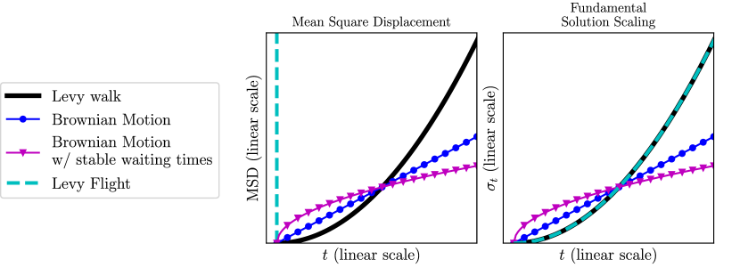
where the left-hand side denotes the variance or second moment of the random variable ; see Figure 1. Given an initial distribution of particles in which then undergo Brownian motion, the distribution of particles in is governed by (1). In other words, diffusing particles described at a microscopic scale by Brownian motion, i.e. by (2) in discrete time, have their distribution in space – a macroscopic property – governed by the heat equation (Meerschaert and Sikorskii, 2011, Section 1.1). This is illustrated in Figure 2.
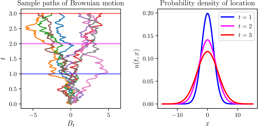
The consistency between this macroscopic description and the microscopic model is illustrated by scaling properties. A necessary property of the Brownian motion model is the second-moment condition (4), which states that on average, particles travel a distance from their initial position after time . This is reflected in the fact that the solution of (1) with initial condition is
| (5) |
which is the normal density (3) with standard deviation . Note that this solution has the property that
| (6) |
Thus, the distribution of plume of particles in this diffusion model spreads out as as time elapses from to , consistent with (4). This scaling of the fundamental solution is illustrated in Figure 1.
The model for normal diffusion reviewed here is also referred to as Fickian diffusion. The heat equation (1) can be derived from the mass conservation with flux term ,
| (7) |
under Fick’s law . As discussed by Schumer et al. (2001), the fractional diffusion equations we introduce below follow from mass conservation with non-Fickian fluxes.
2.1.2 -stable Lévy flights and the fractional Laplacian
Many important systems exhibit diffusive behavior, but do not satisfy the scaling property (4) (Klafter and Sokolov, 2005). This type of diffusion is referred to as anomalous diffusion, as it cannot be described by (2) with normally distributed increments. We desire a microscopic model that generalizes Brownian motion , and a corresponding macroscopic model that generalizes the diffusion equation (1). The first model we propose remains in the framework of a discrete SDE with independent identically distributed (i.i.d.) increments,
| (8) |
but the increments are no longer drawn from a normal distribution. It follows from the central limit theorem that the only way to obtain a microscopic model in this framework that is statistically distinct from , i.e., not equivalent in distribution, is to draw step sizes from a probability density function with infinite variance (Zaburdaev et al., 2015; Meerschaert and Sikorskii, 2011).
We introduce the isotropic -stable random variable . This family of random variables is defined333Several parametrizations of the -stable characteristic function exist. The parametrization (10) is due to Samorodnitsky and Taqqu (1994). See Nolan (2020, 1998) for discussions of alternate forms. most simply by their characteristic function. For a general random variable , the characteristic function is the Fourier transform of the probability density function of , i.e.,
| (9) |
Thus, the characteristic function of the normal random variable is . Generalizing this, the -stable random variable has characteristic function
| (10) |
where
| (11) |
The parameter is referred to as the stability parameter of the distribution, as the center, as the skewness, and as the scale. The isotropic or symmetric -stable distribution therefore has characteristic function
| (12) |
generalizing the characteristic function of the normal distribution with mean and standard deviation and reducing to it when . By definition, the probability density function of can be written
| (13) |
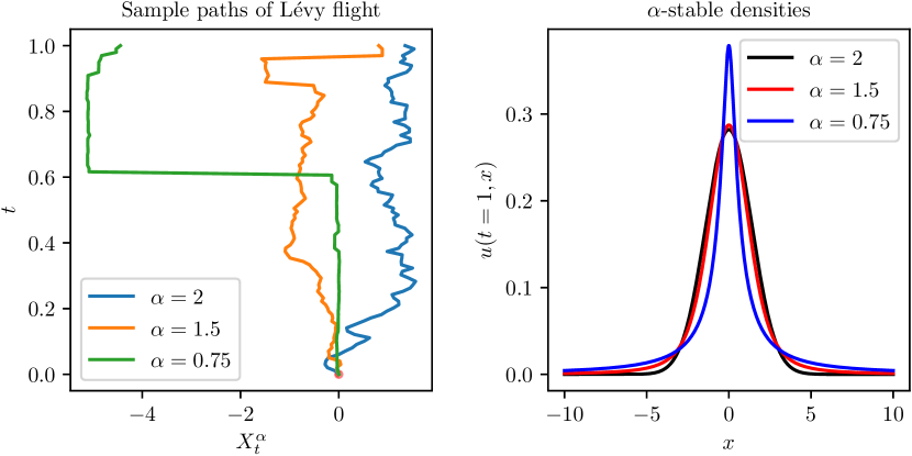
In general, the -stable density does not admit a closed-form expression444Special cases are corresponding to the normal distribution, and corresponding to the Cauchy distribution, and and corresponding to the Lévy distribution., but in the symmetric case where , it has the property that
| (14) |
as discussed in, e.g., Nolan (2020) or Cont and Tankov (2003). In other words, the density exhibits Paretian or power-law tails. This is in contrast to the rapidly decaying square-exponential tails of the normal distribution. In many settings, such tails are informally referred to as being examples of heavy or fat tails (Adler et al., 1998; Haas and Pigorsch, 2009).
Using the isotropic distribution introduced above, we introduce the isotropic -stable Lévy flight by providing the corresponding discrete stochastic process. This is given for with integer by and the rule (Meerschaert and Sikorskii, 2011)
| (15) |
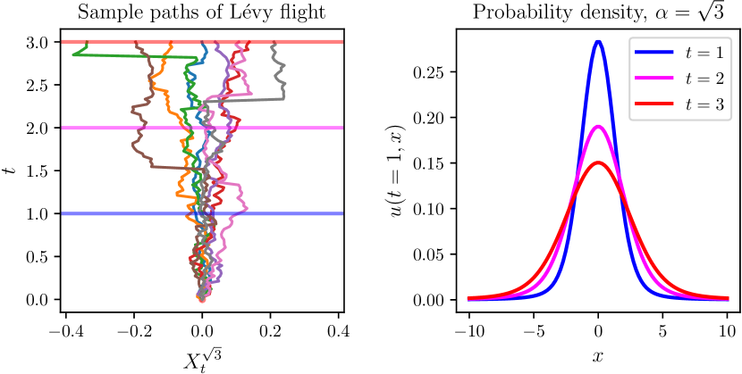
The continuous-time stochastic process for can be thought of as a scaling limit as of the above random walk, and enjoys several theoretical properties such as stability and an extended central limit theorem (Meerschaert and Sikorskii, 2011; Meerschaert and Scheffler, 2001). However, has the property that for , the paths of are almost surely discontinuous, in contrast to Brownian motion – hence the name Lévy “flight”. Given an initial distribution of particles in which undergo -stable Lévy flight, the evolution of the distribution for is governed by the space-fractional diffusion equation (Meerschaert and Sikorskii, 2011, Section 1.2)
| (16) | ||||
as illustrated in Figure 3. The fractional negative Laplacian is defined for and for any dimension as
| (17) |
with
| (18) |
see Lischke et al. (2020). We have defined this operator in any dimension for future reference, although our present discussion only requires the case . Perhaps the simplest characterization of the fractional Laplacian is the Fourier representation,
| (19) |
The simplest case of (16) is the initial condition , in which case the solution is
| (20) |
This is known as the fundamental solution. Although this solution cannot be written in closed form, it satisfies
| (21) |
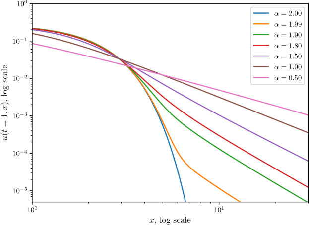
as shown in Meerschaert and Sikorskii (2011, Section 1.2). This illustrates that a plume of particles undergoing isotropic -stable Lévy flight spreads by a factor of as time elapses from to , a faster rate when than the normal rate . Thus, -stable Lévy flight is an example of superdiffusion. The dependence of the above solution as well as sample paths on is shown in Figure 4.
However, since , the tail behavior of the isotropic -stable density implies that the second moment of diverges for ,
| (22) |
with the first moment (the mean) diverging also when Nolan (2020); Zaburdaev et al. (2015). This implies that the variance of -stable motion is not a useful statistic for parameterizing -stable Lévy flight; it bears no useful relationship to . This aspect can be tackled in several ways, motivating the introduction of further fractional-order operators, such as tempered operators and fractional material derivatives discussed below.
We point out several important properties of the fractional Laplacian. From the definition (17), it is clear that , being a constant. The fractional Laplacian also satisfies the semigroup property (Samko et al., 1993). However, one property that is apparent from the definition is that, unlike integer-order derivatives, the fractional Laplacian is a nonlocal operator, i.e. the value of depends on the values of in all of (or , for ). In contrast, the value of any integer-order derivative of at depends only on the values of in an infinitesimal neighborhood of .
2.1.3 The Riemann-Liouville fractional derivatives and asymmetric -stable Lévy flight
The fractional Laplacian (17) was introduced in the previous section as a symmetric or rotation invariant operator for describing the symmetric or isotropic -stable Lévy flight. That model introduced a stability parameter allowing it to generalize normal diffusion, with the scale and center playing similar roles as the standard deviation and mean of the normal distribution. However, the stable distribution also allows for a skewness parameter , with in the symmetric case, which has no analogue in the normal distribution or for Brownian motion. This is due to the central limit theorem, which states that the use of any finite-variance distribution for the i.i.d. increments in (8), no matter how asymmetric, leads to being normally distributed, and therefore necessarily symmetric about the mean. In this section, we introduce the one-sided Riemann-Liouville fractional derivatives as appropriate operators for modeling asymmetric -stably Lévy flights, which are defined by (15) with for nonzero .
The left-sided and right-sided Riemann-Liouville derivatives in are defined, for , as
| (23) | ||||
| (24) |
The texts of Podlubny (1998), Oldham and Spanier (1974), and Meerschaert and Sikorskii (2011) discuss these operators in detail. These derivatives are frequently used in models with and . In connection with initial value problems, the left-sided Riemann-Liouville derivative in time, , is sometimes used with . We have written the definitions (23) and (24) to avoid ambiguities in notation, and clearly show that substitution of the variable occurs after integration and differentiation. An alternative approach is to define Riemann-Liouville fractional integrals separately, as in the right-hand sides of (23) and (24); see Samko et al. (1993).
One quirk of the notation for Riemann-Liouville derivatives in (23) and (24) is the writing of the upper and lower limits of integration and , respectively, as subscripts. While this is suggestive, the result is that the variable of evaluation occurs twice in the notation for each operator. If these derivatives are evaluated at any numerical value of , this value should be substituted in both locations; thus, represents a valid evaluation of the derivatives, but and do not.
With and , the Riemann-Liouville derivatives can be represented in frequency space by
| (25) | ||||
| (26) |
In one dimension, these can be used in the asymmetric diffusion model
| (27) | ||||
which describes anomalous diffusion of independent particles. Here, the positions of each particle at time steps of for integer are governed by (8) with increments being drawn from the asymmetric -stable distribution
| (28) |
Thus, the skewness ranges from when to when . The fundamental solution of (27) is
| (29) |
cf. equation (20).
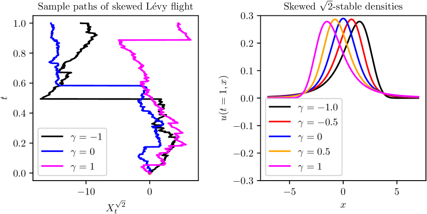
Sample paths of the process just described are illustrated in Figure 6. Note that when , the distribution reverts to the symmetric -stable distribution, and it can be shown in this case that equation (27) reduces to (16); more specifically,
| (30) |
The Fourier representation (25) suggests that the left-sided Riemann-Liouville derivative should be thought of as a fractional power of the operator . However, the correspondence between (27) and (28) makes it clear that to obtain a complete description of -stable Lévy flights in one dimension necessitates two operators, a left-sided and a right-sided operator, which agree with one another when . Our interest is these models lies in the fact that an extended centralized limit theorems hold for processes with i.i.d. increments drawn from distributions with infinite variance, but for which the tails of the density function satisfy Pareto-type conditions as in (14). For such processes, -stable distributions play an analogous role to the normal distribution in the classical central limit theorem; unlike the classical theorem, for full generality, skewed -stable distributions must be included in such a result. See Meerschaert and Scheffler (2001) or Meerschaert and Sikorskii (2011) for a treatment of these results.
We mention how the Riemann-Liouville derivative can be utilized in dimensions . An anisotropic diffusion operator was introduced by Meerschaert et al. (1999) and Benson et al. (2000a) as
| (31) |
Here, denotes a nonnegative measure on the angle in the unit sphere in , and the Riemann-Liouville directional derivative is given by
| (32) |
Benson et al. (2000a) showed that when the measure is uniform, the operator (31) reduces to the fractional Laplacian (17). In higher dimensions and for general measures , the operator (31) plays an analogous role to the operator in the right-hand side of (27), which is in fact a special case of it for . As such, it is used in models of anistropic multivariate -stable Lévy diffusion.
2.1.4 Subdiffusion and the Caputo fractional derivatives
The superdiffusive model introduced above, in which a plume of particles spreads out in space with higher-order rate for , raises the question of whether a process can be constructed which results in diffusion characterized by a lower-order rate than the Brownian rate . In this section, we introduce such a model, constructed as Brownian motion with random waiting times drawn from a skewed stable distribution, supported over positive real numbers with a power-law tail. Here, we step away from the framework of the SDE given by (8). Rather than being defined by a simple time-stepping scheme with i.i.d. increments, the paths of the process are defined by a transformation, or “postprocessing”, of Brownian paths .
We introduce Brownian motion with waiting times, denoted by . The intuition is that the particle paths traced out in space by a discretization of are paths of discretized Brownian motion , but the particles wait at each point of the path for a random time drawn from the totally skewed stable distribution. The operational time , which introduces waiting and replaces linear time , is an inverse stable subordinator. This is a stochastic process in the variable , although we write rather than using a subscript for typographical reasons. This process is constructed by first defining the stable subordinator , and defining to be the inverse process555The definition of in terms of is an example of a right-continuous inverse of an increasing functions. Paths of , thought of as functions of , are nondecreasing, so that each path of constructed in this way is a continuous-from-the-right inverse of the parent path of used to construct it. of . Both and are nondecreasing processes with units of time. In terms of paths, arises from as
| (33) |
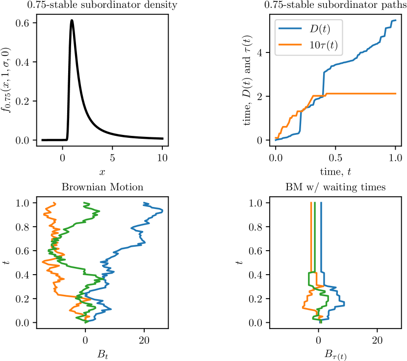
Intuitively, represents a cumulative waiting time process, keeping track of the total time waited by a particle throughout a path, while the inverse represents an operational time, i.e., the time spent traveling. The increments of represent the time waited at each location of a particle before the jump to the next location. More specifically, is a totally skewed -stable Lévy process (28) with stability index , , scale , and center ; see Meerschaert and Sikorskii (2011), Example 5.14. The construction of sample paths of is demonstrated in Figure 7.
The resulting probability density function of ,
| (34) |
for waiting times is supported in nonneagative real numbers. Due to the nonnegative support of the waiting time density, the characteristic function (10) yields the Laplace transform of the waiting time density as
| (35) |
where the Laplace transform is defined as
| (36) |
See Meerschaert and Sikorskii (2011), p. 108 and p. 156 for a discussion. The variance of the process is given by
| (37) |
which is the desired subdiffusive property. Note that the finiteness of the variance does not imply that the normal central limit theorem applies to , which is not equal in distribution to Brownian motion nor to any Lévy process. In fact, is not a Markov processes.
The probability density of Brownian motion with waiting times is governed by the time-fractional diffusion equation,
| (38) | ||||
| (39) |
Here, the Caputo derivative is defined for by
| (40) |
For , this operator is characterized by the simple Laplace transform representation (see Meerschaert and Sikorskii (2011), page 111)
| (41) |
Higher order Caputo derivative can be defined, although the Laplace transforms of the resulting operators involve initial conditions for derivatives of ; see Section 2.3 of Meerschaert and Sikorskii (2011). The Caputo derivative is most frequently utilized as a derivative in time for initial-value problems, with the fractional order .
Before introducing the fundamental solution to the time-fractional diffusion, we introduce the Mittag-Leffler function (Mainardi et al., 2007; Mainardi, 2020)
| (42) |
This Mittag-Leffer reduces to the exponential function when , and has Laplace transform property
| (43) |
which immediately implies that solves the fractional ordinary differential equation
| (44) |
Returning to the diffusion equation (38) with initial condition , applying the Fourier transform in space implies that
| (45) |
which, as shown by Mainardi et al. (2007), yields a solution that can be written
| (46) |
with
| (47) |
being a special case of the Fox-Wright function. Note that . While the fundamental solution above is transcendental, it has the following properties: for , it reduces to the solution (5) of the classical diffusion equation; for , the solution decays faster than exponential and slower than Gaussian; and the second moment of the solution is
| (48) |
Note that the scaling of this second moment is consistent with the scaling of the fundamental solution above.
2.1.5 Continuous time random walks and space-time fractional diffusion
Both the -stable Lévy flight , which led to the space-fractional diffusion equation discused in Section 2.1.3, and Brownian motion with -stable subordinator operational time , which led to the time-fractional diffusion equation discussed in Section 2.1.4, are examples of continuous time random walks (Meerschaert and Sikorskii, 2011). A continuous time random walk (CTRW) allows for a general family of processes in space to be time-changed by a general family of waiting-time processes. To illustrate this concept, we consider the process , which is -stable Lévy flight defined at the discrete level by (28) time-changed by the -stable subordinator process introduced in Section 2.1.4. This models a particle that performs independent jumps drawn from the -stable process, waiting at each point for a random time drawn independently from the -stable subordinator process. As shown by, e.g., Meerschaert and Sikorskii (2011) (Section 4.5), the probability density of this particle position is then governed by a differential equation that is fractional in both time and space,
| (49) | ||||
While intuitive, this result deserves a more detailed outline within the general theory of CTRWs. In the standard CTRW model, particles wait at a location for time drawn from a density function , and jump to a new location by an increment drawn from a density function . The waiting time and jump samples are assumed to be i.i.d., and uncoupled from each other (Zaburdaev et al., 2015; Metzler and Klafter, 2000a; Scalas et al., 2004; Torrejon and Emelianenko, 2018). Thus, the densities and completely determine the CTRW. From the waiting time density , the probability that a particle will remains at any given position for time is
| (50) |
this is referred to as the survival probability of a CTRW particle. Then, given an initial probability density of a particle , which can also be thought of as an initial distribution of an ensemble of independent particles, the following equation was derived by Montroll and Weiss (1965) for the density at later times:
| (51) |
This equation is central to the CTRW theory666This equation was also derived by Scher and Lax (1973a, b) and is referred to as the CTRW equation of Scher and Lax by Klafter and Silbey (1980). Other authors, such as Torrejon and Emelianenko (2018) refer to this as the master equation of a CTRW.. Taking the Laplace transform in time, the Fourier transform in space, and solving for yields the Montroll-Weiss equation (Montroll and Weiss, 1965),
| (52) |
In the case that is the -stable density (28) and is the -stable subordinator density (34), then is given by the analytical formula (10) and by (35), so that the Montroll-Weiss equation represents a closed-form solution of in -space. Unsurprisingly, it is impossible to perform inverse transforms and obtain itself analytically, but can be shown to satisfy (49) using the representations (41) and (25) (Meerschaert and Sikorskii, 2011).
2.1.6 Lévy walks and fractional material derivatives
Superdiffusive -stably Lévy flight exhibits infinite MSD, which is a drawback for certain applications. Related to this is the infinite speed of propagation intrinsic to Lévy flights, i.e., the fact that particles have a nonzero probability of traveling an arbitrary large distance in a unit of time. Brownian motion also suffers from this feature, although this probability of large excursions is so low that MSD remains finite. A prototypical model of superdiffusion that cannot be described by a Lévy flight is ballistic motion, in which particles simply move from an initial configuration in fixed random directions with speed , for all time . A ballistic particle travels a distance in time from an initial position . If reorientations are allowed, then the positions of these so-called sub-ballistic particles in space-time are confined to a ballistic cone
| (53) |
Because the density function of the particle positions is compactly supported, all moments of the position are finite. Such a process cannot be described by Lévy flights.
To capture such behavior, we introduce the Lévy walk model, following Zaburdaev et al. (2015). Such models are based on continuous-in-time motion of particles, rather than instantaneous jumps. A speed of particles in a medium is specified; each particle moves with speed in a chosen direction, before a reorientation event occurs in which the direction changes instantaneously and the particle continues to move with speed before the next direction. Assuming the direction at reorientation is sampled uniformly on the unit sphere, such a walk is determined by a probability density function for the duration of movement . This leads to a survival probability given by (50), with now representing the duration density. Thus, returns the probability that a particle has persisted in a given direction for time , i.e., has not experienced reorientation for time . Similar to the CTRW case, a master equation can be derived for the probability density of the location of the particle in Laplace-Fourier space:
| (54) |
Unlike the master equation for CTRWs, this equation exhibits coupling in Fourier and Laplace variables, representing coupling in space-time777A Lévy walk may be compared to a non-standard CTRW in which waiting times prior to jumps are correlated to the jump length, e.g., propertional to the jump length, so that long excursions are penalized by long waiting times. See . This results in governing equations that are considerably more complex than those of a standard CTRW. For a Lévy walk, is taken to be a Pareto-type distribution,
| (55) |
An asymptotic expansion of and substituted in (56) yields the following approximation for the evolution of the density function of a Lévy walk in Fourier-Laplace space:
| (56) |
Given and , this equation can be inverted to compute , but obtaining a governing equation in is less straightforward from this point on, due to space-time coupling. Sokolov and Metzler (2003) suggest defining a fractional material or substantial derivative
| (57) |
in order to obtain a governing equation for . Recent works, such as those of Chen and Deng (2015), have explored numerical discretizations for these operators.
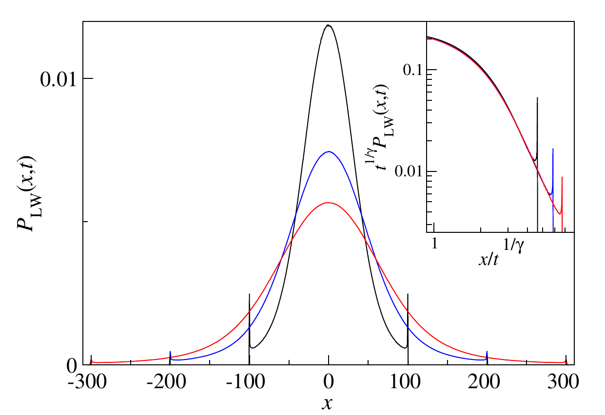
Despite the greater mathematical difficulties related to governing equations, as compared to other fractional models, Lévy walks have been widely used due to the physical nature of finite speed of propagation and finite MSD; see Zaburdaev et al. (2015) for a survey. When , by numerical approximations, it can be seen that evolves from a -distribution with “a central part of the profile approximated by the Lévy distribution sandwiched between two ballistic peaks” that propogate at speed , with an MSD and self-similarity property for large that features a superdiffusive scale factor of Zaburdaev et al. (2015).
2.1.7 Variable-order fractional derivatives
Given the physical meaning within stochastic models of the fractional order in derivatives such as (17), (23), and (40), it is reasonable to expect that these parameters may vary in space and time. Variable-order fractional models are convenient to describe anomalous diffusion in the case of heterogeneous materials or media, or, more generally, when the nature of the diffusion process (subdiffusive, superdiffusive, and classical) changes with space and time. While models with constant fractional order are the simplest and most widely used, some of the model descriptions we discuss in the following sections are improved by the use of a variable fractional order. In recent years, with the purpose of increasing the descriptive power of fractional operators, new models characterized by a variable fractional order have been introduced for both space- and time-fractional differential operators Antil and Rautenberg (2019a); Darve et al. (2021); D’Elia and Glusa (2021); Razminia et al. (2012); Zheng and Wang (2020b) and several discretization methods have been designed Chen et al. (2015); Schneider et al. (2010); Zeng et al. (2015); Zheng and Wang (2020a); Zhuang et al. (2009). The improved descriptive power of variable-order fractional operators has been demonstrated in some recent works on parameter estimation Pang et al. (2020a, 2019a); Zheng et al. (10 Nov. 2020).
Given a function
| (58) |
i.e., a function of space and time, we define variable-order operators as follows. For a function with and , we define the variable-order fractional Laplacian888For more recent works and novel definitions of variable-order fractional Laplacians we refer the reader to Antil and Rautenberg (2019b); D’Elia and Glusa (2021). as
| (59) |
Here, is restricted to take values in . Note that for constant , . For and restricted to , we define the variable-order left-sided Riemann-Liouville fractional derivative as
| (60) |
The right-sided Riemann-Liouville may be defined for variable order in an analogous way. We define the variable-order Caputo fractional derivative, again for taking values in , as
| (61) |
2.1.8 Relationships between processes, fractional models, and applications
To summarize and offer a quick look-up of anomalous diffusion processes, their corresponding fractional models, and applications of each process/model, we have included these relationships in Table 1. This table includes references to the previous sections where each process and model is described, as well as pointers to the applications in the following sections where the models are utilized. We have limited references to applications to only those three areas that we focus on in this article.
| Process | Fractional Model | Section | Application |
|---|---|---|---|
| Symmetric -stable Lévy Flight | Space-fractional diffusion with fractional Laplacian | 2.1.2 | Scalar turbulence §4.2.3. |
| Asymmetric -stable Lévy Flight | Space-fractional diffusion with R.L. derivatives | 2.1.3 | Subsurface flows through fractured media §3.2.1. |
| Brownian Motion with stable Lévy waiting times | Time-fractional diffusion with Caputo derivative | 2.1.4 | Rheology and failure of viscoelastic materials §5.2.1, 5.2.2, 5.2.3, mobile-immobile subsurface flow dynamics §3.2.2. |
| CTRW with stable Lévy jumps and waiting times | Space-and-time-fractional diffusion | 2.1.5 | Subsurface flows through fractured media with trapping zones §3. |
| Lévy Walk | Material derivative with coupled Fourier-Laplace space | 2.1.6 | Superdiffusion as for Lévy flights, but with finite MSD and confined to ballistic cone; see Zaburdaev et al. (2015). |
2.2 Connection to Nonlocal Calculus
Fractional-order differential operators can be viewed as a special case of nonlocal models (Defterli et al., 2015; D’Elia et al., 2020b; D’Elia and Gunzburger, 2013). The intrinsic nonlocality of fractional operators has been illustrated in the previous section; this property describes the fact that fractional-order derivatives of a function at a point typically depend on values of the same function at all points , no matter how large the distance between and may be. An example of this is the formula (17) for the fractional Laplacian.
General nonlocal diffusion (or Laplace) models include integral operators of the form Du et al. (2012, 2013)
| (62) |
with kernels having support in , where the so-called interaction radius is such that . A quick comparison with the integral formula (17) shows that when the kernel is properly selected and , then the fractional Laplacian is formally equivalent to (62) (see D’Elia and Gunzburger (2013) for a rigorous derivation and a discussion).
Nonlocal Laplace operators featuring kernels with bounded support may be preferred to fractional operators for physical reasons when modeling short-range interactions Askari (2008); Silling (2000) as well as mathematical convenience when posing volume conditions, the nonlocal counterpart of classical boundary conditions D’Elia et al. (2020d); Du et al. (2012). The latter reason gives rise to truncated fractional-order derivatives Burkovska et al. (2021); D’Elia et al. (2020b).
General nonlocal models also allow for more flexibility with regards to regularity. Considering diffusion or Poisson’s problems, fractional-order problems exhibit regularity explicitly parametrized by the fractional order Samko et al. (1993); in contrast, nonlocal models involving nonsingular kernel operators lead to problems that impose no regularity on the solution Du et al. (2012) and can be naturally utilized to model fracture dynamics Silling (2000); Silling et al. (2007). Finally, we remark that the relationship between fractional and nonlocal models extends to more general operators than those of diffusion/Laplace type. There is indeed a well-established nonlocal vector calculus (Du et al., 2013; Gunzburger and Lehoucq, 2010), of which fractional-order vector calculus is a special case (see (D’Elia et al., 2020b) for rigorous results where the convergence of truncated fractional gradient and divergence is proven in norm and pointwise).
2.3 A Remark about Numerical Methods for Fractional-Order Models
Over the past two decades, a significant amount of progress has been made in developing numerical methods, ranging from finite-difference/volume schemes to finite-element methods, in addition to a variety of new spectral theories for single and multi-domain spectral methods, obtaining efficient and easy-to-construct smooth/non-smooth basis and test functions. Performing a thorough and inclusive review of all the contributions made in this direction is nearly impossible and out of the scope of present work. Interested readers can find a wide spectrum of research carried out in the context of numerical analysis of fractional models in Almeida et al. (2015); Baleanu et al. (2012); Chen et al. (2016); D’Elia et al. (2020a, c); Diethelm et al. (2005); Furati et al. (2018); Gorenflo (1997); Guo et al. (2015); Li and Zeng (2019); Samiee et al. (2021b); Tarasov (2019); Zayernouri and Karniadakis (2013); Zayernouri et al. (2015, 2022); Zhou et al. (2020), and references therein.
We restrict ourselves to discussing one aspect related to numerical methods, on the computational feasibility of solving fractional models. In the time-fractional case, efficient long-time numerical integration is of interest to capture inherent long time far-from-equilibrium dynamics and to enable the full convolution computations for large-scale systems. To this end, a number of fast time-stepping schemes have been developed during the last 20 years, which greatly reduce the cost of solving fractional models, making them quite comparable to clasical models. These include the fast convolution method by Lubich and Schädle (2002), which reduced the computational complexity of direct finite-difference discretizations of time-fractional models from to , and memory requirements from to , where denotes the number of time steps. High-order extensions of the method were developed Yu et al. (2016); Zeng et al. (2018) and applied to three-dimensional simulations of fluid-structure interactions in cerebral arteries and aneurysms Yu et al. (2016). Among a vast number of works in the literature, we also briefly outline matrix-based schemes, such as fast-inversion approaches Lu et al. (2015) and kernel compression methods Baffet and Hesthaven (2017) for time-fractional problems. For space-fractional FPDEs, adaptive methods and hierarchical matrices approaches have accomplished similar, dramatic reductions in computational complexity and memory costs for solving models Zhao et al. (2017); Xu and Darve (2018); Li et al. (2020). Efficient solvers and preconditioners for the fractional Laplacian were also developed by Ainsworth and Glusa (2017). The point we make is that from two decades of numerical methods development in the field, the current state-of-the-art numerical methods for fractional models produce computational costs comparable to integer-order cases, therefore being timely computational tools to be readily employed in large-scale systems modeled by FPDEs.
3 Anomalous subsurface transport
The accurate prediction at large scales of contaminant transport in both surface and subsurface water is fundamental for efficient management of water resources and hence critical for environmental safety. However, the explicit description of the systems where transport takes place is extremely challenging, especially at large scales, due to the complexity of surface and subsurface environments. In fact, the latter feature heterogeneities that are either hard or impossible to measure and, hence, cannot be described with certainty at all scales and locations of relevance. On the other hand, even when the environment’s microstructure can be captured, numerical simulations of PDE models such as the advection-diffusion equation (ADE) may be prohibitively expensive if conducted at small scales. Furthermore, these same equations that are accurate at small scales fail to predict solutes’ behavior at larger scales, due to the appearance of “anomalous”, or “non-Fickian” behavior Levy and Berkowitz (2003).
Still, in the past, the classical ADE has been broadly utilized as a model for solute transport Decker and Tyler (1999); Erel (1998); Matthess et al. (1991). As thoroughly explained in Neuman and Tartakovsky (2009), in the presence of heterogeneous media, ADEs fail to be accurate at large scales. Such classical models at the coarse-grained scale can be considered accurate only when media properties do not vary rapidly in the neighborhood of a point. Even with mild heterogeneities, quantities defined at large scales vary rapidly enough to be treated as random functions of space and/or time, in which case the ADE becomes an SDE Benson et al. (2001). Interestingly, when treating the ADE’s parameters as stochastic, the ensemble mean concentration through randomly heterogeneous media is generally non-Fickian, i.e. non-classical. This can be observed in a simple manner by performing Monte Carlo numerical simulations. After generating several random realizations of the underlying velocity field, the ADE is numerically solved for each field and the concentration is averaged over all realizations, revealing such non-classical behavior Neuman and Tartakovsky (2009).
In view of the following section where fractional behavior is discussed in the context of turbulence, we point out that the above stochastic theories are closely related to those governing turbulent diffusion. However, while transport in porous media takes place at small Reynolds numbers, the latter take place at large ones. Furthermore, porous velocities depend on hydraulic properties in a known manner, whereas turbulent velocities fluctuate randomly in space–time, making the first uncertainty epistemic (e.g. incomplete knowledge of medium properties) and the second aleatory (i.e. controlled by chance). This makes it easier to reduce the uncertainty in solute transport models by tuning them using hydrogeologic data (see e.g. Tartakovsky (2007)).
In this section we show that Fractional ADEs (FADEs) are appropriate models to describe non-Fickian transport of solutes without the prohibitive burden of resolving the heterogeneities at the small scales explicitly thanks to their integral nature that allows to embed length-scales in the definition of the operator. Before reporting on early works featuring a simple fractional Laplacian model and later works where variable fractional orders are introduced, we dedicate a few words to another nonlocal model, also popular in the literature: the continuous time random walk (CTRW) approach. As we point out later on, these models have similarities and share advantages, the most important of which is perhaps the strong connection to stochastic processes that makes them easier to analyze and interpret.
Fractional subsurface models based on continuous time random walks.
In Section 2.1.5, we discussed the basic concepts of CTRWs, introduced by Montroll and Weiss (1965). We now explain how these models arise in subsurface transport and lead to fractional equations, following Berkowitz et al. (2006); further relevant works in the literature include Berkowitz and Scher (1995, 1998); Boano et al. (2007); Dentz and Berkowitz (2003), and Valocchi and Quinodoz (1989).
To analyze subsurface particles, we begin by examining the solute concentration for a given configuration of particles; refers to the number of particles at a site , normalized by the total number of particles in the system. In the absence of sinks and sources, the solute concentration varies with time at the site by following a stochastic mass balance expression, i.e.
| (63) |
The expression above is known in the literature as (discrete) master equation Oppenheim and K. E. Shuler (1977). Here, is the transition rate at which a particle moves from to , the first term in the sum represents the normalized rate of solute outflow from site to all sites , whereas the second term represents the normalized rate of solute inflow from all sites to . We further assume that the transition rates corresponding to different sites or displacements are statistically independent, i.e. hydraulic and transport properties of porous media and system states (e.g. hydraulic fluxes) lack spatial correlations. This is referred to as statistical incoherence; under this assumption, the ensemble mean concentration , where refers to an average over all possible configurations of the particle system, satisfies the so called generalized master equation, i.e.
| (64) |
As discussed in Berkowitz et al. (2006), this equation is equivalent to a spacetime coupled CTRW equation
| (65) |
with an explicit correspondence between the function and the space-time density function ; see also Klafter and Silbey (1980). If the CTRW is uncoupled, i.e.,
| (66) |
then this equation is equivalent to the CTRW equation (51) discussed in Section 2.1.5. As a result, , in absence of advection, and with and given by the stable distributions specified in Section 2.1.5, is governed by the FPDE (49). This cements the importance of FPDEs in subsurface transport, although in some cases, the incoherence assumption that is required to derive the generalized master equation may not be valid.
A simple and fairly general FADE for subsurface transport under the influence of both advection and anomalous diffusion is the one-dimensional advection and space-time-fractional diffusion equation with constant coefficients (see, e.g., Sun et al. (2020)):
| (67) | ||||
where is the solute concentration, a constant velocity, a constant diffusion coefficient and the fractional order. In Section 2.1.5, we presented equation (49), which is identical to the above equation except for the advection term , as the governing equation for the probability density of a continuous-time random walk. As discussed by Meerschaert and Sikorskii (2011), the inclusion of the advection term corresponds to a stochastic model in which the particle drifts with constant velocity and jumps to the left or the right with density specified by the diffusion term. Thus, when in (2.1.5), the FADE (67) governs the evolution of the probability density
| (68) |
of the skewed -stable process . Comparing to the asymmetric diffusion model in Section 2.1.3, with fundamental solution (29), this density differs only in that the center drifts with velocity . This describes a particle that drifts with velocity and makes jumps to the left or right drawn from the stable distribution (28). More specifically, when particle path ware discretized in steps of , the position of the particle increments by , where is given by (28), at each time step. When , similar to the CTRW model described in Section 2.1.5, this equation governs the probability density of a particle undergoing the process just described, time-changed by the inverse -stable subordinator, again introducing waiting times to the process.
As pointed out by Neuman and Tartakovsky (2009), when , (67) corresponds to a Markovian random walk processes of statistically independent and identically distributed non-Gaussian displacements, and, as such, they can only occur in an uncorrelated velocity field; in hydrology, this can be viewed as a limitation of both CTRW and plain FADEs. Instead, it is possible that variable-coefficient or variable-order models may be able to describe processes associated with statistically non-homogeneous velocity fields. However, we are not aware of a specific theoretical framework that relates variable-coefficient and variable-order FADEs and CTRWs. Nor are we aware of a framework that relates such variable parameters to physical properties of the medium. At present, the only way of estimating such parameters is by fitting the models to observed concentrations and/or mass fluxes, and not by hydraulic data such as hydraulic conductivity, advective porosity or flow parameters such as hydraulic gradients, fluxes and advective porosities Neuman and Tartakovsky (2009).
As discussed in Section 2.1.5, limits of a CTRW with infinite and statistically independent waiting times leads to time-fractional FPDEs. A physical mechanism that would result in time-fractional derivatives in a FADE is particle trapping due to media heterogeneities Compte (1996); Giona and Roman (1992). Such models are discussed in Section 3.2.2.
We conclude this section with advantages in using FADEs as opposed to more general CTRW models. First, it is well-known Meerschaert et al. (2001) that FADEs can account for source and boundary terms and velocity dynamics can be easily included by an additional velocity equation, which leads to a velocity-concentration coupled system. Furthermore, even though not thoroughly explored, model fitting for FADEs is a computationally less challenging task than for general CTRWs, due to the smaller number of parameters to fit.
3.1 Evidence of fractional behavior in the presence of heterogeneity
In this section we provide two examples of fractional behavior of solute concentration. We start by considering a highly heterogeneous environment and then we show that even in circumstances where a classical behavior is expected, i.e. in the absence of heterogeneities, the macroscopic solute concentration behaves nonlocally and is described by a FADE.
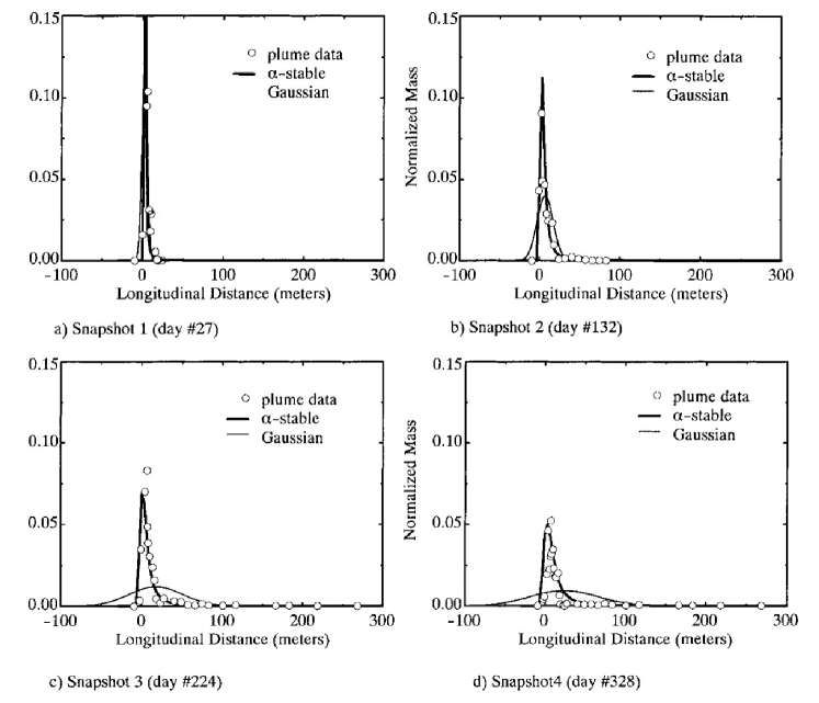
Fractional behavior is most readily seen in transport through heterogeneous media. The first experiment we discuss studied subsurface transport of tritium in a highly heterogeneous environment such as the MADE site, located on the Columbus Air Force Base in northeastern Mississippi. This unconfined, alluvial aquifer consists of generally unconsolidated sands and gravels with smaller clay and silt components. Irregular lenses and horizontal layers were observed in an aquifer exposure near the site Rehfeldt et al. (1992). Detailed studies characterizing the spatial variability of the aquifer and the spreading of the conservative tracer plume for the experiment conducted at the beginning of the 90’s can be found in Boggs et al. (1993). Benson et al. (2001) used (67) to model particle concentration; model parameters were determined a priori by tuning them on the basis of measurements (we refer to Benson et al. (2001), Sections 4.2 and 4.3, for a detailed description of the calibration process). In Figure 9 we report four snapshots of the normalized longitudinal tritium mass distribution. These plots are obtained by numerical integration of the analytic solutions of both the classical ADE and the FADE. These distributions clearly indicate that the fractional model outperforms the classical one.
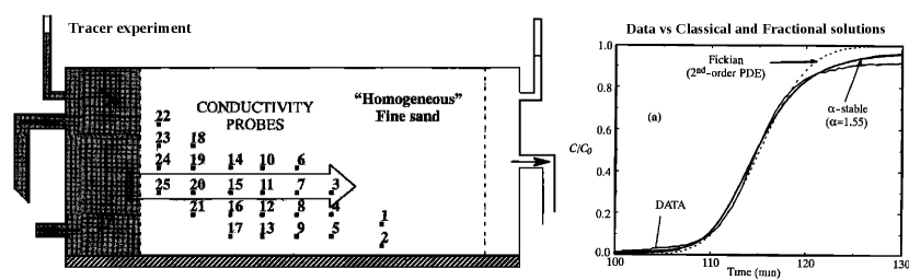
Strong heterogeneity, however, is not necessary to observe fractional behavior. Increasing experimental evidence suggests that in laboratory experiments where the media is “constructed” as nearly homogeneous, the observations are nevertheless consistent with anomalous transport, see, e.g., Levy and Berkowitz (2003); Zhang and Lv (2007). In fact, some authors even argue that transport in the subsurface is always anomalous Zhang et al. (2013). Benson et al. (2000a) analyzed a test case where the tracer’s concentration was intuitively expected to follow a classical ADE. They considered a one-dimensional tracer test in a laboratory-scale, 1 meter, sandbox, constructed with very uniform sand in an effort to minimize heterogeneity, see Figure 10, left. In other words, the sandbox was designed and built using as homogeneous a porous medium as possible by following the set up in Burns (1996). Simple tracer tests, conducted to estimate the transport characteristics of the sand, indicated the appearance of non-classical breakthrough curves (BTCs, i.e., plots of the concentration in time at a fixed point downstream of a source) with heavy tails, similar to -stable solutions. This behavior was likely due to channeling within smaller and smaller grains that resulted from sand emplacement through standing water and from cracked and intact surface clays on the sand particles Benson et al. (2000a). In Figure 10, right, a comparison conducted in Benson et al. (2000a) between BTCs obtained with the classical ADE and the FADE equation shows the agreement of the latter with measured BTCs at a specific location. While in this Figure the differences between classical and fractional behavior are not striking as in Figure 9, they are still noticeable.
We also mention that evidence of anomalous behavior and its successful description by FADEs has been observed in unsaturated soils Zhang et al. (2005), saturated porous media Zhou and Selim (2003), streams and rivers Deng et al. (2004, 2006a), and overland solute transport due to rainfall Deng et al. (2006b).
3.2 State of the art: a progression of fractional models for subsurface transport
As described at the beginning of this section, classical diffusion does not take into account long-distance spatial and time correlations. The anomalous movement of particles in the subsurface, however, depends on both far upstream/downstream concentrations (resulting in space-fractional equations (Cushman, 1991; Cushman et al., 1994; Schumer et al., 2001; Zhang and Lv, 2007)) or past conditions (resulting in time-fractional equations (Cushman et al., 1994; Dentz and Tartakovsky, 2006; Dentz et al., 2004; Schumer et al., 2003a)). Considering only the movement of solute particles in an infinitesimal neighborhood, as in the classical diffusion model of Brownian motion, is too restrictive for the complexities of groundwater pore spaces or trapping zones in natural streams. More specifically, the presence of preferential paths in hydrologic domains results in high-velocity zones (superdiffusion), whereas the presence of trapping regions results in low-velocity zones where the particles “wait” before they return to the higher velocity zone (this concept is also known in the literature as the distinction between immobile and mobile zones) (Sun et al., 2020).
In this section we review fractional models of increasing complexity for anomalous subsurface transport. While the simpler models are viable choices in the presence of a low degree of heterogeneity, as this degree increases, more sophisticated models are required to obtain reliable predictions. We first present early works featuring a one-dimensional space FADE with constant coefficients and constant fractional order. Next, we extend this model to the case of variable coefficients and generalize it to the multi-dimensional setting. We then present two types of one-dimensional time FADEs and conclude the section with a very general model featuring both space and time fractional derivatives of variable order. For all these models, we refer to Section 2.1 for their mathematical details and interpretation in the context of stochastic processes.
3.2.1 Spatial fractional derivatives
We introduce the constant-coefficients, constant-order spatial FADE in one dimension introduced in Benson et al. (2000a) and provide details regarding its parameters in relation to solute transport. The solute concentration at point and time , , satisfies the equation
| (69) |
where is the average plume velocity, is a fractional diffusion coefficient999The units of are given by where is the fractional order, L indicates space and T indicates time. that controls the rate of spreading, (dimensionless) is the fractional order, and determines the skewness . Solutions can be positively () or negatively () skewed, whereas they are symmetric when , for which the sum of the Riemann-Liouville derivatives results in the fractional Laplacian The fractional order codes for the heterogeneity of the velocity field, with a higher probability of large velocities as it decreases towards one Clarke et al. (2005). We recall that for the FADE reduces to the traditional advection-diffusion equation (ADE) for groundwater flow and transport. The FADE above was introduced for the first time by Benson et al. (2000b) to model scale-dependent dispersivity in fitted groundwater plumes. In this paper the authors observed that, given a data set of solute concentration, the fitted parameter grows with time when the classical ADE is used; such evidence of superdiffusion is an indicator that a space-fractional model is preferable. Indeed, in subsequent works, see e.g. Benson et al. (2001), the same authors show that the FADE allows the same data set to be fit with a constant-coefficient model such as (67), where does not vary over time. From a particle perspective, the combination of left-sided and right-sided RL derivatives allows a solute particle to jump to any point in the domain; this simple concept was used by Schumer et al. (2001) to provide a derivation of (67) using an Eulerian interpretation of the particles’ behavior.
The Grünwald-Letnikov discretization technique.
A standard discretization technique used in the FADE community for the approximation of the left-sided and right-sided RL derivatives (23) and (24) in (67) is the shifted Grünwald-Letnikov (GL) finite difference formula introduced by Meerschaert and Tadjeran (2004). The GL scheme is based on the following identities:
| (70) | ||||
where the GL weights are given by
| (71) |
The GL approximation of the one-dimensional FADE is obtained by truncating the summation in (70). The temporal derivative and the classical first-order spatial derivative can be obtained by standard time discretization schemes for PDEs. The discretizations (70) lead to stable time-stepping schemes and clearly highlight the nonlocal nature of fractional derivatives. Such discretizations also illustrate the potential for higher computational and memory cost entailed by solving FPDEs using direct approaches, which are greatly reduced using more the advanced numerical methods described in Section 2.3.
FADEs with variable coefficients on bounded domains.
In a heterogeneous porous medium, at a scale where the geological character of the medium changes with location, the constant-coefficient model (67) is insufficient for accurate and reliable predictions. A first step towards a more accurate model is introducing space dependence in the material parameters and . Furthermore, in practical settings, simulations of solute transport must be confined to bounded domains, so that it becomes mandatory to establish ways to prescribe nonlocal boundary conditions that guarantee existence and uniqueness of solutions. In the literature there are at least three variants of the FADE with space-dependent coefficients Kelly and Meerschaert (2019): the fractional-flux ADE (FF-ADE), the fractional-divergence ADE (FD-ADE), and the fully fractional divergence ADE (FFD-ADE). In this review we focus on the former because of its resemblance to classical advection-diffusion equations101010We refer to Kelly and Meerschaert (2019) for more details regarding the FD-ADE and FFD-ADE models.. For this model, we formulate the associated equation on bounded domains.
The FF-ADE model in the one-dimensional domain is derived from the classical conservation of mass equation
| (72) |
where the flux is given by the following constitutive equation Schumer et al. (2001)
| (73) |
Here, the first term is the advective flux that models the average drift of contaminant particles, whereas the second and third terms are the dispersive fluxes, which model large particle jumps in the left and right directions, respectively. Note that, because we consider the bounded domain , the integrals in the the left- and right-sided derivatives are “truncated” at and , respectively. Furthermore, since the RL derivatives in the definition of the flux have exponent . The resulting FF-ADE corresponds to the models proposed in, e.g., Zhang et al. (2006). We point out that, as described in detail in Kelly et al. (2019), Caputo derivatives as the ones introduced in Section 2.1 can also be used in place of RL derivatives in the definition of the flux (leading to what is referred to as Caputo flux).
The restriction of the FADE to a bounded domain requires the prescription of appropriate boundary conditions to guarantee that equation (72) is well-posed. We consider two types of boundary conditions: reflecting and absorbing. Using the flux function defined in (73), we can identify a reflecting (or no-flux) condition by setting the diffusive part of the flux equal to zero at the boundary, i.e. . As an example, the reflecting boundary condition on the right boundary corresponds to
Instead, absorbing boundary conditions correspond to prescribing a zero “Dirichlet” condition at the boundary, i.e.,
Clearly, these conditions can be mixed resulting in absorbing/reflecting boundary conditions on either the left or right boundary of the domain. It is important to note that, in the absence of advection, the no-flux (reflecting) condition implies that the total mass is conserved, see Proposition 2.3 by Kelly et al. (2019). We also mention that a new space-fractional model with variable advection and diffusion coefficients for anomalous, anisotropic transport has been proposed by D’Elia and Gulian (2021, Submitted).
Multidimensional FADEs
The multidimensional version of equation (67) was proposed by Meerschaert et al. (1999) and further analyzed in Benson et al. (2000a). For defined as in (31), we have that for the concentration of a solute is described by the following law:
| (74) |
where is the average solute velocity and is the fractional diffusion coefficient. In Meerschaert et al. (1999) the operator corresponding to (31), is introduced via inverse Fourier transform, i.e.
Here, is a -dimensional unit vector, is the wave vector and is the spatial Fourier transform of . Note that the coefficient can be embedded in the measure (even when it depends on the space variable). As for the one-dimensional constant-coefficient equation (67), the multidimensional FADE can also be extended to the variable-coefficient case. Furthermore, in the special case of jumps occurring only along the standard coordinate vectors , it is possible to derive fundamental solutions to (74). Finally, the special case of uniform measure over the unit sphere corresponds to an advection-diffusion equation where the diffusion term is given by the standard fractional Laplacian operator .
3.2.2 Temporal fractional derivatives
The time-FADE, used to model particle trapping in heterogeneous porous media, is characterized in a jump process perspective by long waiting times between jumps. As discussed in Section 2.1.4, this equation replaces the first-order time-derivative in an ADE with a time-fractional derivative of either RL or Caputo type. In this section, we review two popular time-FADEs: the time-FADE (with RL derivatives) and the fractional mobile-immobile equation (with Caputo derivatives), also known as FMIM.
Time-fractional advection-diffusion equation
The time-fractional advection-diffusion equation (time-FADE) was introduced in the works by Zaslavsky (1994) and, independently, by Liu et al. (2003). In one dimension, it is given by
| (75) |
where the first term is the Caputo derivative defined in (40) on the half-axis. The units of the velocity parameter are and the ones of the diffusion coefficient are , where L denotes units of space and T units of time. Note that, in the literature, is often denoted by , where plays the same role as . Furthermore, as pointed out at the beginning of this section, the time-FADE can be seen as the scaling limit of a CTRW. It is possible to obtain representations of solutions to (75) by subordination, i.e. via randomization of the time variable by the inverse stable subordinator Meerschaert and Straka (2013).
Fractional mobile-immobile equation
The fractional mobile-immobile (FMIM) model proposed by Schumer et al. (2003b) is a generalization of the classical mobile-immobile (MIM) model Coats and Smith (1964). The latter, in its classical definition, partitions the solute concentration into a mobile phase, , and an immobile phase, and equates the divergence of the total flux of the mobile concentration to a weighted sum of the time rate of change of each phase, i.e.
| (76) |
where , being and the porosities of the immobile and mobile phases. The relationship between and is then given by one or more coupled mass transfer equations, resulting in the following relationship
| (77) |
where indicates the convolution operation and is a memory function. The FMIM model in Schumer et al. (2003b) defines as the power function with . By noting that
the combination of (77) and (76) results in the time-FADE
A CTRW model for the FMIM model, was developed by Benson and Meerschaert (2009); here, waiting times experienced by solute particles in the immobile phase are modeled by a power law (as for the time-FADE). As regards the realism of the assumptions underlying this model, power-law waiting times have also been observed in river transport studies by Haggerty et al. (2002) and Schmadel et al. (2016).
3.2.3 Variable-order FADEs
Constant-coefficient and constant-order models are invaluable basic tools for the analysis of complex engineering systems such as the flow through the subsurface; however, they are unable to evolve between different physical behaviors, i.e. they cannot capture transitions between diffusive regimes. These transitions are caused by the fact that solutes in the subsurface diffuse through porous, fractured, layered and heterogeneous aquifers, whose structure changes with space as well as time. This leads to anomalous diffusion characterized by a variable-order scaling of the MSD. While the variable-coefficient models described above allow for more flexibility with regards to scaling properties, a more direct way to address this need is with variable-order models. Several recent works have explored the use of variable-order operators in the context of subsurface modeling and other applications. The use of these operators becomes particularly important in the presence of complex media that feature a hybrid anomalous mechanism Patnaik et al. (2020). As an example, we can exploit variable-order fractional operators, like the ones introduced in Section 2.1.7, when the nature of the transport processes transitions across very different underlying physical phenomena such as transitions from sub-diffusive flow to diffusive flow, and from diffusive flow to super-diffusive flow Atangana and Kilicman (2014); Kobelev et al. (2003); Sokolov and Klafter (2006); Sun et al. (2009, 2010, 2014). Note that these complex transport processes have been observed experimentally in various fields; for fluid flow through porous media we mention, e.g., the works of Gerasimov et al. (2010) and Obembe et al. (2017).
A complete variable-order fractional model was proposed by Sun et al. (2014) and further explored by Pang et al. (2017) for the description of the same MADE data set introduced at the beginning of this section. The one-dimensional variable-order time-space FADE is given by
| (78) |
where the variable-order derivatives are defined as in Section 2.1.7.
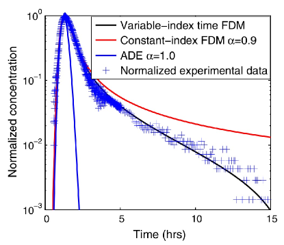
To confirm the improved accuracy of models such as the one in (78) we report in Figure 11 a comparison, conducted by Sun et al. (2014), of a classical model, a constant-order fractional model and a variable-order fractional model. Here, the authors consider concentration data from the field experiment conducted at the Grimsel test site Berkowitz et al. (2008) where uranine, a fluorescent dye, was injected into a shear zone as a tracer and its concentration was measured at an extraction well away from the injection site. The BTC of uranine, measured at the extraction well corresponds to the blue crosses in the figure. The authors compare the following models: the classical advection-diffusion equation, corresponding to and in (78), the constant-order time FADE with and , and the variable-order time FADE with , , and . BTCs in the figure show that the classical ADE model is not capable to depict the tailing/subdiffusive behavior, whereas the constant-order time FADE underestimates the late time decay, which features classical behavior. The choice of and in the variable-order time FADE is based on the following considerations: first, the measured BTC has a fast-increasing early time tail, implying a Gaussian-type of particle jump that corresponds to . Second, the heavy late-time tail suggests a time-dependent that should be less than 1 at early times (subdiffusive) and should slowly convergence to 1 at late times (classical diffusion). The corresponding solid black BTC clearly captures the variable diffusion behavior of the normalized concentration.
3.3 Future directions in anomalous subsurface modeling
In the previous sections we provided evidence of the occurrence of anomalous behavior in subsurface transport even for a low degree of heterogeneity and we have shown that FADEs can be accurate models when properly tuned. However, the identification of an optimal fractional model for a specific setting (e.g. for specific hydraulic properties) is not trivial and has not been thoroughly explored in the literature. One of the main challenges in this context is the fact that model parameters cannot be directly related to media properties, as carefully explained by Neuman and Tartakovsky (2009). Furthermore, often times, it is hard or nearly impossible to collect solute measurements, so that only a very small set of data that are sparse in time and space and potentially affected by noise is available. Yet, in this context, FADEs have the advantage, compared to other models for subsurface transport, of having only a handful of parameters to tune, i.e. the identification problem consists in discovering a small set of parameters such as the diffusivity and the fractional order.
Only a few works in the literature have addressed this problem. In the context of highly heterogeneous settings, we mention the work by Pang et al. (2017) where the authors propose to use multi-fidelity Bayesian optimization to discover variable-order fractional operators for the advection–diffusion equation (78) from field data in the MADE data set mentioned at the beginning of this section. Other recent works addressing a similar learning problem for fractional operators include optimization-based approaches such as the one used by Burkovska et al. (2021), fractional/nonlocal physics-informed neural network approaches such as those of Pang et al. (2019b, 2020a) and operator-regression techniques such as the one developed by You et al. (2021). It is important to keep in mind that the inverse problem of parameter identification may multiply the cost of numerical computations, which is already higher in direct approaches than classical methods due to the integral nature of the operators involved and to the strong singularities that require adaptive quadrature rules. Thus, together with the development of frameworks for learning models, the efficient numerical methods mentioned in Section 2.3 take on an additional importance in model discovery.
4 Turbulence
Richard P. Feynman described turbulence as the most important unsolved problem in classical physics Eames and Flor (2011), a problem that stands today. By “turbulence”, we refer to the three-dimensional and highly vortical fluid motions characterized by stochastic perturbations in pressure and flow velocity, and caused by excessive kinetic energy in areas of fluid flow that overcome the “damping effects” of the fluid’s viscosity. The onset of turbulence can be predicted by the dimensionless Reynolds number Re, a ratio of kinetic energy to viscous damping in the fluid flow. Yet, the question remains of what mathematically governs the evolution of a turbulent flow and whether it is feasible to fully simulate turbulent flows by means of numerical methods.
In 1970, Emmons (1970) reviewed the possibilities for computational fluid dynamics, concluding: “… the problem of turbulent flows is still the big holdout. This straightforward calculation of turbulent flows – necessarily three-dimensional and unsteady – requires a number of numerical operations too great for the foreseeable future." After almost a decade, however, the field of direct numerical simulation (DNS) of turbulence was established with successful numerical simulations of wind-tunnel flows at moderate Re by Hussaini and Voigt (2012); Karniadakis et al. (1993); Kim et al. (1987); Orszag and Patterson Jr (1972). These early computational developments were based on employing a Newtonian fluid assumption and applying the principles of conservation of mass, momentum, and energy to an infinitesimally small fluid element or parcel; see e.g., Chorin et al. (1990); Temam (2001); White and Majdalani (2006). This led to the derivation of the Navier-Stokes and energy equations, emerging as a set of convective nonlinear PDEs that govern the evolution of fluid velocity/temperature fields in turbulence. In this context, assuming some proper (random) initial/boundary conditions, one can discretize the governing equations and solve for the “entire degrees of freedom of turbulence” in the physical and parametric (stochastic) space.
The great challenge is that in practice, DNS becomes prohibitively expensive, especially at high Re, more so in complex geometries. Hence, one of the main goals in turbulence modeling has been to systematically lower the total number degrees of freedom to a manageable level, at the cost of reducing the accuracy of turbulence predictions. This approach has been mainly centered around the overarching theme of ensemble averaging the set of PDEs representing the various scalar and vector turbulence fields; see e.g., Lumley and McMichael (1995); Wilcox et al. (1998). This gives rise to new mathematical terms in the averaged or filtered governing equations, known as turbulence closure terms that can only be modeled as they are essentially unknown. When the entire time and length scales of turbulence are averaged, the Reynolds Averaged Navier-Stokes (RANS) equations are obtained, solely describing the mean-flow dynamics of turbulence. Alternatively, if one applies a mathematically well-defined low-pass filter to the Navier-Stokes equations, the resulting filtered governing equations describe the large-eddy dynamics of turbulence, where only small-scale subgrid dynamics need be modeled; this is referred to as large eddy simulation (LES). The common approach in the literature for modeling closure terms of any kind has been based on the use of classical local differential operators. More specifically, the majority of turbulence models have been constructed based on Boussinesq’s turbulent viscosity concept (Pope, 2001), in which one assumes that the turbulent stress tensors are proportional to the local gradient of mean velocity at any point. The proportionality coefficient, referred to as turbulent viscosity, is to be inferred from data.
The impetus for the fractional models we describe in this section is that the small-scale dynamics of turbulence are statistically anomalous, i.e., non-Markovian and non-Fickian, so that nonlocal closure models emerge as appropriate tools. Employed at the continuum level, fractional models therefore capture anomalous features in the small-scale stochastic subgrid dynamics of turbulence. The mathematical modeling of turbulence must address the fact that nonlinear interactions between the turbulence structures and motions create statistically complex phenomena that lead to a variety of anomalous features, including multi-power-law scalings in space-time, rare events, short-to-long range coherent motions, and enhanced turbulent mixing. These features urge better and novel understanding of the underlying nonlocal closure terms that appear as a result of the ensemble averaging or filtering of the governing equations. The nonlocal mode of thinking has the potential to shift the turbulence modeling paradigm and achieve a new level of physical and statistical consistency compared to classical approaches. This is especially true at high Re, for which a proper and efficient framework that unites computational, mathematical, and statistical aspects was not available until recently.
4.1 Evidence of Fractional Behavior in Turbulence
An intuitive concept of nonlocality and memory effects was been established by Eringen and Wegner (2003), where a point within a fluid field (medium) is influenced by all points of the body at all past times. Coherent random motions and the spatially turbulence spots structures inherently give rise to intermittent signals with self-similarities, sharp peaks, heavy-skirts, and skewed distributions of velocity increments. Such statistical features have been well-observed experimentally even in the context of most canonical problems, e.g., grid turbulence, in which the skewness factor negatively appears and the Kurtosis factor strongly exceeds three, emphasizing the non-Gaussian character of statistics (see e.g., Davidson (2015)). Moreover as demonstrated by Egolf and Kutter (2020) (page 92), nonlocal effects appear even in the context of turbulent fields obtained numerically solving the Navier-Stokes equations. Such widespread statistical measures indicate the non-Markovian and non-Fickian nature of turbulence, and they are the consequence of nonlinear and coherent vortical effects that occur in a wide spectrum of length and time scales. Therefore, nonlocal interactions cannot be ruled out of modern turbulence physics. These considerations are particularly timely; in fact, we can now benefit from the spectrum of modern nonlocal and fractional modeling tools reviewed in Section 2.1, equipped with well-established mathematical/statistical theories, that enable us to take such nonlocal/history effects into account with physical consistency and mathematical rigor.
Furthermore, averaging entire spatial scales as in RANS models or applying a spatial filter to the Navier-Stokes and energy equations as in LES models would make the underlying physical nonlocality in the corresponding closure terms in RANS models and the subgrid turbulent fluctuations in LES models even more pronounced. This sheds lights on why turbulence modeling is a nonlocal task and further motivates the development of “nonlocal closure models” that can properly address and incorporate the underlying memory and long-range effects. Specifically, in what follows, we present a DNS study, recently presented by Akhavan-Safaei et al. (2021), that introduces new statistical measures and highlights the nonlocal character of subgrid scale dynamics in the context of scalar turbulence.
4.1.1 The case of scalar turbulence subgrid dynamics
An ideal LES is such that the true, filtered turbulent intensity is captured accurately through a robust subgrid scale (SGS) modeling that is physically and mathematically expressive. In fact, the LES equations include closure terms that directly link the correct evolution in time of turbulent intensity to the nature of the SGS closure and its modeling. Here, as a canonical problem, we consider the advection-diffusion (AD) equation
| (79) |
in which denotes the molecular diffusion coefficient of the passive scalar, and the imposed mean scalar gradient is taken to be uniform as , where is a real-valued constant. In the LES representation of the scalar turbulence, multiplying both sides of the “filtered” AD equation by , the filtered scalar field , yields the time-evolution of the filtered turbulent intensity as
| (80) |
Here, denotes the -th component of the residual, SGS scalar flux defined as . Employing the filtered continuity equation and the chain rule for differentiation, we obtain
Applying the ensemble-averaging operator, , on (4.1.1) returns a transport equation for the filtered scalar variance, . Akhavan-Safaei et al. (2021) considers the case of homogeneous turbulent velocity and scalar fields, in which . Defining the filtered scalar gradient as , the time-evolution of the filtered scalar variance takes the following form
| (82) | ||||
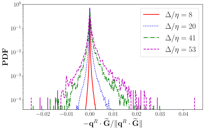
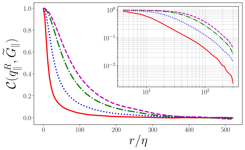
In (82), denotes the turbulent transport of filtered scalar variance while represents the production of resolved scalar variance by the uniform mean scalar gradient, and is the resolved scalar variance dissipation due to the molecular diffusion. Unlike these three terms, (representing the SGS production of resolved scalar variance) is the only contributing term in (82) that contains the effects of the SGS scalar flux. Therefore, as pointed out earlier, understanding the true statistical nature of is essential for the SGS modeling and precise evaluation of the resolved scalar variance in the LES. This examination of might be viewed both from single-point and two-point statistics as discussed by Meneveau (1994) in the context of the LES for homogeneous isotropic turbulent flows. We focus on the two-point statistics of the SGS production of resolved scalar variance. This quantity is well represented in terms of the following normalized two-point correlation function
| (83) |
where denotes the spatial shift from the location . Moreover, the probability density function (PDF) of the SGS production of scalar variance normalized by its -norm i.e., , is a novel statistical measure for studying the statistical behavior of and yielding a more comprehensive insight into the SGS modeling.
Let be the eddy turnover time. By taking a large sample space over of this stationary process (after resolving the passive scalar field for ), the PDF of the normalized SGS production of filtered scalar variance is computed for four different filter widths, . These computations, shown in Figure 12(a), demonstrate that as becomes larger, the PDF exhibits broader tails. Emergence of this tail behavior implies that as the filter width increases, long-range spatial interactions become stronger and more pronounced Akhavan-Safaei et al. (2020). Motivated by this observation, a two-point diagnosis of the SGS scalar production of the filtered variance as defined in equation (83) would be another statistical measure shedding light on the long-range interactions in addition to the filter width effects. Considering as the direction along the imposed mean scalar gradient and representing the directions perpendicular to the imposed mean gradient, we focus on the evaluation of .
Here, one case takes and and takes the average of the resulting two-point correlation functions. Due to the statistically stationary turbulence, such procedure is performed for 20 data snapshots that are uniformly spaced over (on the same spatio-temporal data, used to compute the PDFs); hence, the time-averaged value of is obtained. Figure 12(b) illustrates this two-point correlation function extending over a wide range of spatial shift, , and evaluated at four filter widths similar to the ones utilized in Figure 12(a). This plot quantitatively and qualitatively reveals that as increases, greater correlation values between the SGS scalar flux , and filtered scalar gradient are observed at a fixed . These spatial correlations are significant both in the dissipation and also inertial subranges.
This confirms substantial nonlocal effects in the true SGS dynamics, which need to be carefully addressed in the SGS modeling for LES.
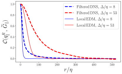
A popular and fairly simple approach for modeling the SGS scalar flux is Eddy-Diffusivity Modeling (EDM). In EDM, the main assumption is that the SGS scalar flux is proportional to the resolved scale scalar gradient (i.e., the conventional locality assumption) as
| (84) |
and is the proportionality coefficient. Obviously, EDM is a local modeling approach by construction. Computing while is approximated with EDM, one can compare it with its true value as shown in Figure 12(b). Figure 13 illustrates such comparison for two filter widths, , and it reveals that in both of the cases local EDM substantially fails to predict the conspicuous long-range spatial correlations observed in the true two-point correlation values. This evidence strongly suggests the adoption of more sophisticated, nonlocal mathematical modeling tool that goes beyond conventional SGS modeling.
4.2 State of the art: fractional turbulence modeling
In what follows, we present the history and state of the art in fractional turbulence modeling, including nonlocal RANS, fractional eddy-viscosity modeling, fractional scalar turbulence LES modeling, in addition to tempered fractional LES SGS modeling for turbulence.
4.2.1 Nonlocal RANS models: a narrative survey
Recall that most of turbulence models are built based on Boussinesq’s turbulent viscosity concept. Thus, one conventionally assumes that the turbulent stress tensors are proportional to the symmetric part of local mean velocity gradient at any point (i.e., strain-rate tensor). Hence, the corresponding proportionality coefficient, known as the turbulent viscosity, emerges as the unknown turbulence model parameter in
| (85) |
Prandtl (1942) in 1942 aimed to move beyond this local constraint by introducing the extended mixing length concept for the first time. The corresponding new model was a great migration from locality to nonlocality, but did not achieve a remarkable success as it did not significantly improve accuracy. Afterward, he parametrized the primitive model in a way that the mixing length was taken to be greater than the (differential) length-scale of the problem, including a higher (second-order) Taylor expansion term. This strategy was analogous to adding a “weak sense of (short-range) nonlocality” to the model. This was regarded as a weak nonlocal model in the sense that the stress term was still in the form of Boussinesq’s and the relation with the strain rate tensor in the same point was collinear. However, von Karman insisted on the consideration of the common local mixing length, which is generated by the local flow conditions and suggested considering the mixing length in terms of two succeeding derivatives Egolf and Kutter (2020). Bradshaw (1973) in 1973 showed that Boussinesq’s hypothesis fails over curved surfaces and noted that form of the stress-strain relations was the main cause of this failure. It should be mentioned that there were some important developments mostly based on polynomial series, compared to the Boussinesq-type modeling including the works done by Spencer and Rivlin Spencer and Rivlin (1958, 1959), Lumley (1970) and Pope (1975); however, a noticeable lack accuracy both in terms of physics and mathematics emerged as additional second- (and higher) order tensor series developments were demanded, where an interplay between predictability and practicality remained an open question.
As indicated in Section 2.1, Brownian motion can serve as a statistical model for the spread of a cloud of particles the continuum limit of which is a parabolic integer-order diffusion equation. Generalizing this approach to heavy-tailed processes such as Lévy processes can model the intermittency in turbulent flow signals and through a heavy-tailed central limit theorem converge to an anomalous diffusion equation with fractional derivatives in space and/or time West (2016a). This suggests that employing fractional-based Reynolds stresses would be a proper model for the turbulent diffusion term. In a pioneering work by Hinze et al. (1974) in 1974, the authors described the memory effect in a turbulent boundary layer flow. They utilized the experimental data produced downstream of a hemispherical cap, attached to the lower wall of channel geometry. They demonstrated that when one computes eddy-viscosity using Boussinesq’s theory in the lateral gradient of the mean flow and turbulence shear-stresses, there is a huge non-uniform distribution that exists in the outer region of the boundary layer. Interestingly, we see a nonlocal expression for the gradient of the transported field in a novel approach by Kraichnan (1964) in the same year (1974), for the scalar quantity transport. Afterward, fractional-order models based on the RANS approach were offered in Chen (2006); Epps and Cushman-Roisin (2018); Egolf and Hutter (2017a); Hamba (1995, 2005). Most of these works are using Green’s functions based on the residual velocity to provide the expression for the Reynolds stress or scalar fluxes.
One of the main contributions for the development of nonlocal models has been done by Egolf and Hutter Egolf and Hutter (2017b); Egolf and Kutter (2020). They started from Lévy flight statistics and generalized the zero-equation local Reynolds shear stress expression to a nonlocal and fractional type. The method is based on Kraichnanian convolution-integral approach and utilizing different weighting functions. Using the mentioned weighting functions, one can make a bridge between the first-order gradient of the common eddy diffusivity models and the mean velocity difference term. The proposed model is based on the four distinct steps that can be followed conveniently to replace a local operator with a nonlocal one. In reality, the final proposed model is a more general and extended version of Prandtl’s zero-equation mixing length and shear-layer turbulence models. The proposed model is called Difference-Quotient Turbulence Model (DQTM), given by
| (86) |
Although well-motivated and presented as somewhat of a generalization of classical models, such models have not been thoroughly tested against established integer-order models, and their practical efficiency in addressing the nonlocalities have not been adequately examined. Recently, a series of remarkable developments in fractional turbulence modeling gave a new and practical perspective on employing fractional calculus in turbulence, and introducing new statistical measures that directly reveal where classical approaches have room for modernization and enhancement. In what follows we review such cutting edge approaches.
4.2.2 Fractional eddy-viscosity models
Recently, Di Leoni et al. (2021) developed a new nonlocal eddy viscosity-based model (see equation (87) below) that can be applied in both isotropic and anisotropic turbulent flows. They obtained a proper two-point stress-strain rate correlation structure for a priori testing the developed model and performed tests based on the high-resolution DNS data set for the homogeneous isotropic turbulence (HIT) and the channel flow canonical test cases.
The investigation of the model performance is set based on the necessary conditions for any LES approach in providing the accurate two-point statistics of the filtered quantities in the terms of correlations and spectra. The proposed model is given by:
| (87) |
where the derivative operators and are both of order respectively in and directions, however, they are employed as the truncated Caputo derivative variations, still being the convolution of the first derivative of velocity with respect to an inverse power-law kernel with index , however, over a truncated (compact) integral support, forming a finite nonlocality horizon, for the purpose of lowering the computational cost.
Several numerical tests conducted in Di Leoni et al. (2021) indicated that the new model provides a better correlation between the filtered rate of strain rate and subgrid scale stress tensor. Specifically, this model predicts the long tails in the ground-truth subfilter stress–strain-rate correlation functions. However, other conventional local eddy viscosity-based models like classical Smagorinsky, that corresponds to , miss this important feature as they decay faster (see Figure 14).
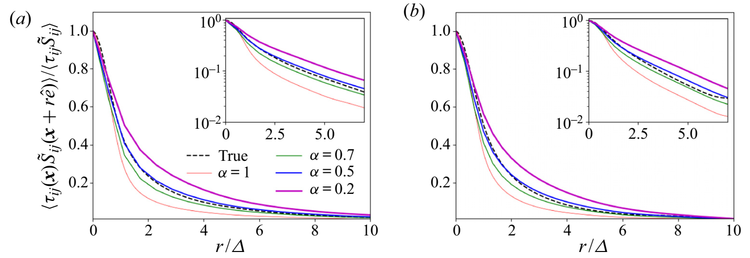
In addition to the significantly better capability in the prediction of the long-tail interactions in the new model, the probability density functions of the dissipation quantities for the HIT flow using the box filtering approach, are matching much better than the local model. The local model predictions are purely dissipative and with no tail behavior, which is contrast with the ground-truth DNS data sets. Moreover, effects of the different parameters in the LES procedure have been analyzed including filter size, filter type, wall distance for the channel flow case, and integration radius.
Alternatively in studying the turbulent transport and mixing, kinetic Boltzmann theory has shown a rich and promising ground based upon principles of statistical mechanics, which by construction is well-suited for the stochastic description of turbulence at microscopic level Harris (2004). In the following, the fundamental sources of nonlocal closure and the SGS modeling for the residual passive scalar flux are studied at the kinetic Boltzmann transport framework. Our objective is to derive a nonlocal eddy-diffusivity SGS model at the continuum level. In what follows we present three recent development of LES SGS where the SGS small motions are modeled by the BGK kinetics transport.
4.2.3 Fractional LES SGS modeling for scalar turbulence
Statistical description of LES is well-represented through incorporating a filtering procedure into the kinetic Boltzmann transport. For the purpose of passive scalar transport, applying a spatially and temporally invariant filtering kernel, , onto the distribution function linearly decomposes that into the filtered, , and the residual, , components. Therefore, filtering the BGK equation results in the following filtered BTE (FBTE) for the passive scalar:
| (88) |
where represents the generic Boltzmann filter size. As elaborated by Girimaji (2007), the nonlinear nature of the collision operator, , prohibits the filtering kernel to commute with; thus, it initiates a source of closure at the kinetic level in FBTE (88). Defining , this closure problem is manifested in the following inequality,
| (89) |
The identified closure requires proper means of modeling so that one can numerically solve the FBTE (88). A common practice is to approximate this closure problem with a modified relaxation time approach that is described in detail in Sagaut (2010). Despite the success of this approach in some applications, it is not physically consistent with the filtered turbulent transport dynamics Girimaji (2007). Nevertheless, here we manage to adjust this inconsistency by looking at the nonlocal effects arising from filtering the Maxwell distribution function, , and model them with proper mathematical tools. Considering the spatial filtering kernel with the filter-width , and applying it on the Maxwell equilibrium distribution as
| (90) |
where . Subsequently, by rewriting the right-hand side of the passive scalar FBTE (88) into the following form
| (91) |
the unclosed part is structurally multi-exponentially distributed and maybe approximated by a power-law distribution model as we propose
| (92) |
where denotes an -stable Lévy distribution that is mathematically designed based on heavy-tailed stochastic processes and replicate the power-law behavior Applebaum (2009); Meerschaert and Sikorskii (2019). The corresponding macroscopic continuum variables associated with the filtered (79) are obtained in terms of the filtered distribution functions, and , as
| (93) | |||||
| (94) |
According to the microscopic reversibility of the particles that assumes the collisions occur elastically, the right-hand side of (88) equals zero Saint-Raymond (2009). Therefore,
| (95) |
Since we are working with spatial filtering kernels, ,
| (96) |
By plugging (96) into (95), we obtain that
| (97) |
where
| (98) |
The corresponding filtered passive scalar flux is obtained through a sequence of step-by-step derivations as
| (99) |
and the divergence of residual scalar flux is derived as the fractional Laplacian of the filtered total scalar concentration,
| (100) |
where is a model coefficient with the unit []. The filtered AD equation for the total passive scalar concentration, developed from the filtered kinetic BTE with an -stable Lévy distribution model, yields a fractional-order SGS scalar flux model at the continuum level. The aforementioned filtered AD equation reads as
| (101) |
Through a proper choice for the fractional Laplacian order , the developed model optimally works in an LES setting. Applying the Reynolds decomposition and considering the passive scalar with imposed uniform mean gradient, equation (101) fully recovers the filtered transport equation for the transport of the filtered scalar fluctuations, .
4.2.4 Fractional/tempered-fractional LES models for fluid turbulence
For some pedagogical purposes, we first presented the case of fracitonal LES SGS modeling for scalar turbulence. However, this new paradigm in LES modeling actually began prior to Akhavan-Safaei et al. (2021). Samiee et al. (2020) developed the first ever fractional LES model for homogeneous isotropic turbulent flows as
| (102) |
being based upon on the derivation of fractional Laplacian closure term in the spatially filtered Navier-Stokes equations when employing a Lévy stable distribution as the equilibrium model in the filtered BGK kinetic transport equation. In Samiee et al. (2021a), they later developed a generalized version of this earlier model (suitable for incorporating data with tailored/truncated tails). Employing rather a tempered Lévy stable distribution in the kinetic level this time gave rise to the formulation of the tempered fractional LES closure term as
| (103) |
forming a novel, data-friendly and expressive tempered fractional Laplacian SGS model for turbulence. They also showed that the newly developed nonlocal models can better recover the non-Gaussian statistics of subgrid-scale stress motions while they are being employed at the continuum level.
4.3 Future directions in fractional turbulence modeling
Laval et al. (2001) analyzed the effects of the local and nonlocal interactions on the intermittency corrections in the scaling properties in three-dimensional turbulence. They observed that nonlocal interactions are responsible for the creation of the intense vortices and on the other hand, local interactions are trying to dissipate them. Inspired by the mentioned observations, they came up with a new turbulence model that accounts for both the local and nonlocal interactions for the study of intermittency. In their proposed model, the large and small scales are being coupled by nonlocal interactions using a multiplicative process and additive noise along with a turbulent viscosity model for the local interactions. The results of the new model qualitatively cover the previously observed anomaly and intermittency aspects.
In the context of nonlocal turbulence modeling, Song and Karniadakis (2018) proposed a variable-order fractional model for wall-bounded turbulent (mean) flows. They represented the Reynolds stresses with a nonlocal fractional derivative of variable-order that decays with the distance from the wall. Interestingly, they found that this variable fractional order has a universal form for all Re and for three different flow types, i.e., channel flow, Couette flow, and pipe flow. In addition to the aforementioned fully-developed flows, they modelled turbulent boundary layers and discussed how the streamwise variation affects the universal curve (see also (Song and Karniadakis, 2021) for a follow-up work). Later, Pang et al. (2020b) proposed a nonlocal truncated operator with spatially variable order, which is suitable for modeling wall-bounded turbulence, e.g. turbulent Couette flow. They showed that nonlocal physics-informed neural networks (nPINNs) can jointly infer the variable order, exhibiting a universal behavior with respect to Re, a finding that can contribute to better understanding of nonlocal interactions in wall-bounded turbulence. In terms of memory-effects (i.e., nonlocality in time), Parish and Duraisamy in Parish and Duraisamy (2017) developed a dynamic SGS model for LES, based on the Mori–Zwanzig (MZ) formalism. This closure model was constructed by exploiting similarities between two levels of coarse-graining via the Germano identity of fluid mechanics and by assuming that memory effects have a finite-temporal support. This work suggests future studies on using time-fractional derivatives in turbulence models.
The aforementioned developments are practically interesting, mathematically exciting, and algorithmically robust. They encourage the field of research in turbulence to open its arms towards the new wealth of mathematical developments in both theory and practice of fractional modeling. Inevitably, further systematic studies and developments of nonlocal turbulence models are needed (both numerically and experimentally) in order to achieve the charming blend of enhanced accuracy and lowered cost in realistic applications. On this note, we end this section by emphasizing that the non-Markovian/non-Fickian nature does not relax in compressible flows (i.e., variable density problems). Therefore the idea of developing generalized fractional turbulence models for transonic-to-hypersonic flows is a new and ripe venue for research, in which the existing sense of classical thermodynamics can become fundamentally non-equilibrium and nonlocal.
5 Fractional constitutive laws in material science
Accurate modeling of evolving material response and failure across multiple time- and length-scales is essential for life-cycle prediction and design of new materials. While the mechanical behavior of a number of standard engineering materials (e.g., metals, polymers, rubbers) is quite well-understood, a significant modeling effort still needs to be conducted for complex materials, where microstructure heterogeneities, randomness and small scale physical mechanisms (such as collective behavior) lead to non-standard and, at times, counter-intuitive responses. Two examples are bio-tissues and natural materials (e.g. biopolymers), which are multi-functional products of millions of years of evolution, locally optimized for their hosts and environment, and constrained by a limited set of building blocks and available resources Imbeni et al. (2005); Wegst et al. (2015). These materials possess unprecedented properties at low densities, especially due to their hierarchical and multi-scale structure, leading to a wide spectrum of behaviors, such as power-law viscoelasticity, viscoplastic strains under hysteresis loading, damage, failure, fatigue, fractal avalanche ruptures and self-healing mechanisms.
The main motivation for fractional materials modeling is the power-law fingerprint arising in microstructures undergoing anomalous diffusion, observed in a range of complex materials. Such microstructures often display a fractal nature with sub-diffusive dynamics, e.g., of entangled polymer chains, and defect interactions such as dislocation avalanches, cracks and voids. Such non-exponential behavior cannot be accurately modeled by integer-order, linear viscoelastic models, which require arbitrary arrangements of Hookean/Newtonian elements and introduce a limited number of exponential (Debye) relaxation modes that, at most, represent a truncated power-law approximation Bagley (1989). While these approximations may be satisfactory for short times and engineering precision, they often result in high-dimensional parameter spaces and still lack predictability outside the experimental time/length-scales, often requiring recalibration. In this context, fractional operators become appropriate and natural modeling choices, since their integro-differential operators naturally utilize power-law convolution kernels, coding self-similar microstructural features in a reduced-order mathematical language with smaller parameter spaces (similarly to the case of anomalous transport, see Section 3). This fact allows accurate and predictive modeling, in an efficient manner, of bio-tissues Meral et al. (2010); Magin and Royston (2010); Craiem et al. (2008); Suki et al. (1994); Djordjević et al. (2003); Nicolle et al. (2010); Puig-de Morales-Marinkovic et al. (2007) and polymers Winter and Mours (1997); Ketz et al. (1988); Baghdadi et al. (2005); Sollich (1998) for multiple time-scales.
In this section we review fractional models for materials undergoing power-law behaviors, termed anomalous materials, in a range of non-equilibrium and path-dependent responses. We start with linear viscoelasticity, introducing the basic modeling building block, known as Scott-Blair element that models a single power-law response and can be combined to incorporate more complex behaviors. In harmony with the previous sections, we will emphasize on potential multi-scale connections, stochastic processes, and thermodynamic consistency. After providing evidence of cases where fractional behavior/power-laws appear as intrinsic qualities in a number of systems, we report on the state-of-the-art models incorporating multiple physical mechanisms.
Fractional viscoelasticity: rheological building blocks.
We start with the Boltzmann superposition integral for linear viscoelasticity, obtained from the linear superposition of infinitesimal step strains applied to a viscoelastic material Mainardi and Spada (2011):
| (104) |
where and denote, respectively, the strain rate and stress. The convolution kernel , is a relaxation function, directly related to stress relaxation experiments under step strains. It is traditionally modeled through combinations of Hookean springs and Newtonian dashpots, yielding a multi-exponential relaxation in the form . In this particular choice of kernel, (104) is equivalent to a multi-term ordinary differential equation (ODE).
Relaxation experiments across multiple time- and frequency-scales indicate that anomalous materials exhibit memory effects in time for stress/strain responses, which translates into a single power-law scaling in the form , with . This indicates that, contrary to exponential relaxation forms, there is a spectrum of relaxation times arising from the material microstructure Jaishankar and McKinley (2013), for which standard ODE models (e.g. generalized Maxwell model in creep/relaxation representations) would require a large number of parameters.
The fundamental fractional rheological building block element, termed Scott-Blair (SB) model, is obtained by substituting the power-law kernel into (104), leading to the following form:
| (105) |
which is equivalent to the Riemann-Liouville fractional derivative if the function is sufficiently well behaved at Podlubny (1998). While this equivalence is satisfied for semi-infinite domains, the choice of Riemann-Liouville and Caputo definitions matter when we introduce a causal strain history and switch the lower limit of (105) from to , which leads to two different fractional Cauchy problems. For the Caputo definition, we have Mainardi and Spada (2011):
| (106) |
On the other hand, when employing Riemann-Liouville derivatives, we obtain:
| (107) |
where we remark that problem (106) is more commonly adopted due to the appearance of integer-order ICs, while both aforementioned problems are equivalent in the presence of homogeneous ICs. The SB element provides a constitutive interpolation between a Hookean spring () and a Newtonian dashpot (). The unique parameter pair codes snapshots of a dynamic process instead of an equilibrium state of the system Jaishankar and McKinley (2013). Consequently these properties are only associated with equilibrium states in the limit cases for the fractional order . We remark that although the FDE (106) utilizing the Caputo definition is widely employed to represent the SB element in the literature, the pioneering works on anomalous rheology modeling are attributed to Gerasimov (1948) in 1948, introducing a similar power-law convolution operator as (105), which may be referred in the literature as the Gerasimov-Caputo derivative Valério et al. (2014). We refer the reader to Valério et al. (2014); Mainardi (2012) for more details on the historical context of fractional derivatives in visco-elasticity.
Mechanistic and thermodynamic interpretations.
Apart from the Boltzmann integral representation (104), characterized by an integro-differential nature, the SB element can also be obtained through a continuous arrangement of canonical, Hookean and Newtonian elements, both from their constitutive and free-energy levels Schiessel and Blumen (1993); Lion (1997), making the notion of SB elements intrinsically incorporating an infinite number of relaxation times more evident. In Schiessel and Blumen (1993), a hierarchical ladder-like structure of standard Maxwell viscoelastic elements was employed. This structure led to a coupled system of ODEs, which had an infinite continued fraction (a recursion of fractions) representation in terms of the Maxwell model constants in the Laplace domain. Then, applying an inverse Laplace transform, a fractional stress-strain relationship was recovered for homonegeous initial conditions, therefore equivalent to both forms (106) and (107). In Lion (1997), an isothermal Helmholtz free-energy density was derived for the SB element from the elastic energies of a discrete-to-continuum arrangement of standard Maxwell branches, obtaining the following form for the free-energy as a function of the strain:
| (108) |
where denotes the relaxation spectrum. Therefore, (108) represents the amount of available elastic energy to perform work from the SB element in the time domain, which cannot be directly inferred from (106) and (107). Naturally, the two limit cases for are when , and when . Furthermore, under suitable thermodynamic constraints, it is shown that the SB element is thermodynamically admissible and that the Caputo representation of (107) can be derived from (108) under continuum mechanics arguments.
Energy decoupling in the frequency domain.
Similar to the aforementioned representations, power-law structures also appear in viscoelastic dynamic properties and rheological experiments in the frequency domain Jaishankar and McKinley (2013), such as the complex shear modulus, defined as the ratio between the Fourier transform of stresses and strains:
| (109) |
where denotes the frequency. The term is the storage modulus, and denotes the loss modulus, i.e., the stored and dissipated energy per cycle, respectively. Employing definition (109) into (107), the dynamic modulus of the Scott-Blair element is obtained Schiessel et al. (1995):
| (110) |
which provides a clear storage/loss decomposition, with the value of determining whether the material of interest is predominantly dissipative for certain frequency ranges.
Relationships to material microstructure and stochastic processes.
The mechanistic origins of macroscopic power-law behaviors in complex materials are due to spatio-temporal anomalous sub-diffusive processes Metzler and Klafter (2000b) in fractal micro-structures. We focus on the temporal case, in which the MSD of microstructural constituents follows a nonlinear scaling in the form . Bagley and Torvik (1983) provided a relationship between the complex shear modulus obtained from the Rouse theory of polymer dynamics. They started with the result of Rouse’s theory for the shear modulus, i.e.
| (111) |
where denotes the number of molecules per unit volume, is the number of monomers in the polymer chain, represents the absolute temperature, is Boltzmann’s constant. The term denotes the relaxation times of the solution, which was approximated as , which is valid when the number of submolecules is large. The terms and denote, respectively, the steady-flow viscosities of the solution and solvent. They further worked on Rouse’s results, and by assuming the polymer chains and to be sufficiently large, obtained the following power-law form for the dynamic shear modulus:
| (112) |
After applying the inverse Fourier transform, the above relationship leads to a Riemann-Liouville representation between stresses-strains with . Similar observations were also reported for utilizing a Zimm model, where the inclusion of hydrodynamic interactions lead to a fractional order . Glöckle and Nonnenmacher (1993) showed that fractional relaxation can be modeled by a special type of CTRW describing a trapping problem due to entanglements of polymer chains, thus slowing down the relaxation process. In their work, the random walkers, i.e., the particles, are considered as packages of free volume that allow conformational reorientations of chain segments, thus leading to relaxation. They obtained a waiting time distribution of such particles through a Fox-Wright representation in the form:
| (113) |
for which the leading term indicates that the CTRW waiting time corresponding to fractional relaxation exhibits a Lévy-type decay in the form .
Connecting dynamic viscoelasticity across scales.
A connection between power-laws propagating from micro- to macro-rheology was proposed in Mason (2000), with the use of a Generalized Stokes-Einstein Relation (GSER) for spheres undergoing generalized Langevin dynamics in a viscoelastic medium:
| (114) |
which is valid for spheres of radius comparable to the length-scale of the embedding medium. Here, the dynamic shear modulus is related to a velocity memory function from Langevin dynamics. Among a variety of representations for the GSER, (114) assumes a power-law structure of the MSD with exponent , which approaches zero when the sphere is confined by elastic structures present in the complex fluid. Such power-law representation also reduces errors near the frequency extremes when employing Laplace and Fourier transforms.
Physical interpretation of fractional orders.
Despite existing connections between micro- and macro-rheological properties, the physical interpretation of the emerging fractional orders has been elusive. More recently, a connection between the fractional order and the fractal dimension of the material microstructure was made by Mashayekhi et al. (2019), where the authors extended the Zimm theory of polymer dynamics to fractal media as a bridge between the meso- and macro-scales. They showed that the fractional order is a rate-dependent material property that is strongly correlated with the fractal and spectral dimensions in fractal media.
5.1 Evidence of fractional behavior
We provide a few examples of fractional/power-law behaviors in viscoelasticity and micro/macro-scale plasticity. We start with two examples in viscoelasticity of solid-like and fluid-like natures in which fractional modeling is more appropriate, both with better fits and a reduced number of model parameters.
Viscoelastic rheology.
Jaishankar and McKinley (2013) calibrated classical and fractional Maxwell models to the four orders-of-magnitude relaxation data for highly anomalous butyl rubber data from Blair et al. (1947) (Fig.15 (a)), and observed that the three-parameter fractional Maxwell model provided an excellent fit to the experimental data, while a multi-exponential, integer-order Maxwell model required six parameters to provide a satisfactory fit. Moreover, using the calibrated fractional relaxation parameters they obtained an accurate prediction of the creep compliance for the same material, especially for long-time behavior. The second experiment from Jaishankar and McKinley (2013) concerns the dynamic properties of acacia gum, a commonly used food preservative. In this case, they compared a four-parameter fractional Maxwell model with a single mode (three-parameter) standard Maxwell model (Fig.15(b)) and demonstrated that while the fractional Maxwell model captures a complex Cole-Cole behavior, its integer-order counterpart is unable to even estimate the qualitative response.

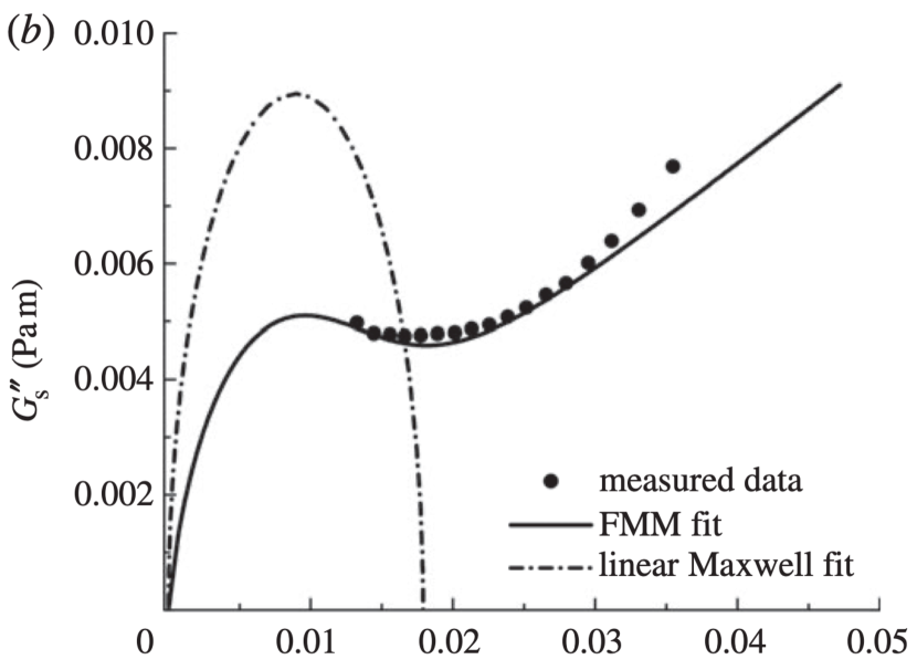
We note that other factors, such as material heterogeneity can introduce multiple power-law relaxation regimes.
In Stamenović et al. (2007) Stamenović measured the complex shear modulus of cultured human airway smooth muscle and observed two distinct power-law regimes separated by an intermediate plateau. Kapnistos et al. (2008) found an unexpected tempered power-law relaxation response of entangled polystyrene ring polymers, compared to the usual relaxation plateau of linear chain polymers. Such behavior was interpreted through self-similar conformations of double-folded loops of ring polymers, instead of the reptation observed in linear chains.
Power-law plasticity.
The creep behavior of human embrionic stem cells (ESCs) under differentiation was studied by Pajerowski et al. (2007) through micro-aspiration experiments at different pressures. The cell nucleus demonstrated distinguished visco-elasto-plastic power-law scalings, with for the plastic regime, independent of the applied pressure. It is discussed that such low power-law exponent arises due to the fractal arrangement of chromatin inside the cell nucleus.
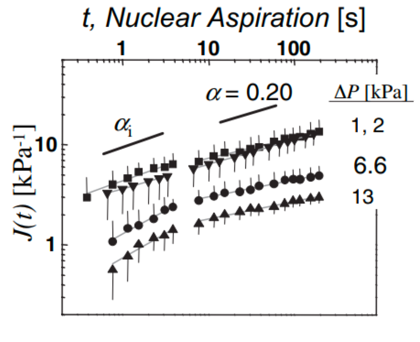
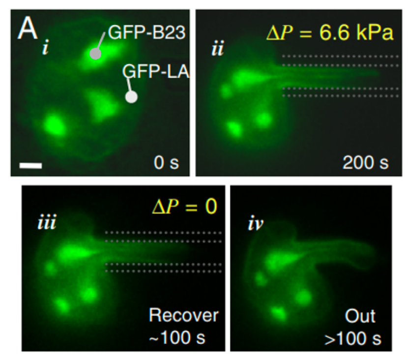
Studies on force-induced mechanical plasticity of mouse embrionic fibroblasts were performed by Bonadkar et al. (2016). It was found that the viscoelastic relaxation and the permanent deformations followed a stochastic, normally-distributed, power-law scaling , with values ranging from to . The microstructural mechanism of plastic deformation in the cytoskeleton is due to the combination of permanent stretching and buckling of actin fibers.
As for evidence of power-laws in failure of crystalline materials, Richeton et al. (2005) investigated the emergence of intermittency and dislocation avalanches in polycrystalline plasticity through acoustic emission experiments on ice under creep compression. Their findings demonstrate that different from the scale-free, close-to-critical dislocation dynamics of single crystals Miguel et al. (2001), the introduction of average grain sizes from the polycrystal microstructure led to a tempered power-law distribution of avalanche sizes. While the exponential tempering cutoff changes with , the authors observed a constant power-law scaling for all samples.
Connections to stochastic processes.
Although the sub-diffusive MSD coefficient is observed in a variety of studies for complex materials and fluids, there exist different interpretations on the underlying stochastic processes linked to the sub-diffusive physics, e.g., crowding or caging effects in cells and polymers. Szymanski and Weiss (2009) utilized fluorescence correlation spectroscopy (FCS) of proteins immersed in crowded dextran solutions and reported a distribution of MSD coefficients with average , and compared this experimental finding with recovered distributions of MSD coefficients for simulated fractional Brownian motion (fBm), obstructed diffusion (OD), and CTRWs. Their findings indicated that the recovered distributions for fBm and OD matched the experiments, while the recovered distributions for CTRW-induced diffusion, with average did not agree well with the data due to ergodicity breaking. Weber et al. (2010) studied the subdiffusion of bacterial chromosomal loci in viscoelastic cytoplasm and further concluded that fractional Langevin motion to be more likely than CTRW and OD, due to the presence of ergodicity and a negative velocity auto correlation function. Regarding polymers, Wong et al. (2004) studied the thermal motion of colloidal tracer particles in entangled actin filament (F-actin) networks, under different concentrations and network mesh sizes. They observed a sub-diffusive behavior when the tracer particles radius were comparable to the network mesh size, and suggested that such anomalous behavior happens due intermittent caging behavior, followed by sudden infrequent jumps with a power-law distribution of caging times in the form .
5.2 State of the art: Anomalous materials modeling
As observed in Section 5.1, experimental evidence suggests that complex material behavior may possess more than a single power-law scaling in the viscoelastic regime, particularly in multi-fractal structures, which are characteristic of cells Stamenović et al. (2007) and biological tissues Vincent (2012), due to their complex, hierarchical and heterogeneous microstructure. For such cases, a single SB element is not sufficient to capture the observed behavior, even if linear viscoelasticity holds. Furthermore, material nonlinearity due to large strains and additional physics such as plasticity, damage and failure require more advanced rheological models, which could have full or partial fractional nature. In this section we refer to a class of fractional models in the literature, classified by rheology type and nature of the corresponding FDEs. We acknowledge that rheology is a vast field with a large number of different types of material behavior, and here we limit our review to visco-elasto-plasticity, damage mechanics and failure.
5.2.1 Viscoelasticity
Linear viscoelasticity.
We start by introducing two natural extensions of the SB viscoelastic model through serial and parallel combinations. The first one is the fractional Kelvin-Voigt (FKV) model, which is given by a parallel combination of SB elements, and relates the stresses and strains in the following additive form Schiessel and Blumen (1993):
| (115) |
where the fractional orders are such that , and , are the associated pseudo-constants. The corresponding relaxation function also assumes additive form of two SB elements:
| (116) |
where contrary to the scale-free relaxation behavior of a single SB element, since we assume , the FKV model possesses two time-scale dependent power-law regimes, given by as and as , which characterizes a transition from faster to slower relaxation regimes. We note that this quality allows the FKV model to describe materials that reach an equilibrium behavior for large times when , which is intuitive from the mechanistic standpoint as one of the SB elements becomes a Hookean spring.
Through a serial combination of SB elements, we obtain the fractional Maxwell (FM) model Jaishankar and McKinley (2013), given by:
| (117) |
with , and two sets of initial conditions for strains , and stresses . We note that in the case of non-homogeneous initial conditions, there needs to be compatibility conditions Mainardi and Spada (2011) between stresses and strains at . The corresponding relaxation function for this building block model assumes the more complex Miller-Ross form Jaishankar and McKinley (2013):
| (118) |
where denotes the two-parameter Mittag-Leffler function, defined as Mainardi and Spada (2011):
| (119) |
Interestingly, the presence of a Mittag-Leffler function in (118) produces a stretched exponential relaxation for smaller time-scales and a power-law behavior for larger time-scales. The asymptotic behaviors are given by as and as , indicating that, contrary to the FKV model, the FM model has a constitutive transition from slower-to-faster relaxation. We refer the reader to McKinley and Jaishankar (2013); Bonfanti et al. (2020) for a number of applications of the aforementioned models. Additionally, we notice that both FKV and FM models are able to recover the SB element with a convenient set of pseudo-constants, or naturally reveal the necessity of standard rheological elements according to available data. Furthermore, we also outline more complex building block models that produce more flexible responses, including three to four fractional orders, such as the fractional Kelvin-Zener (FKZ), fractional Poynting-Thomson (FPT), and fractional Burgers (FB) models. We refer the reader to Bonfanti et al. (2020); Schiessel and Blumen (1993) for more details on such models.
Numerical Discretization.
A well known numerical scheme to discretize the time-fractional Caputo derivatives of order in (115) and (117) is the implicit L1-difference scheme by Lin and Xu (2007). Let points on a uniform time-grid be defined as with time steps of size . The discrete time-fractional Caputo derivative of a function evaluated at is given by:
| (120) |
where with the constant only depending on , and the convolution weights . The above expression can be rewritten and approximated as:
where the so-called history term is given by:
| (121) |
We note that although the above discretization is of practical and simple implementation, there exist many sophisticated numerical methods for fractional Cauchy equations that employ faster schemes, and also address non-smooth, nonlinear and stiff problems. We also emphasize that employing the kernel into the Boltzmann representation for the aforementioned models may be impractical, since one would need other specialized numerical methods that are model-dependent, and would require evaluations of Mittag-Leffler functions.
Nonlinear Viscoelasticity.
Fractional linear viscoelastic models are suitable candidates to describe the anomalous dynamics of a number of materials undergoing small strains. However, under large strains, material nonlinearities induce stress/strain dependencies on the relaxation behavior. One alternative to incorporate such nonlinearity is through quasi-linear viscoelasticity (QLV) Fung (2013), which replaces by a multiplicative decomposition between a reduced relaxation function and an instantaneous, nonlinear elastic tangent response:
| (122) |
with and . Fractional approaches to QLV were developed by Doehring et al. (2005) for arterial valve cusp and by Craiem et al. (2008) for arterial wall viscoelasticity. In the latter, a reduced, fractional Kelvin-Voigt-type relaxation function was employed, with pseudo-constant , and nonlinear exponential form , with constant . Therefore, the fractional QLV formulation is able to capture not only linear/nonlinear instantaneous stress response, due to the rearrangement and alignment of fibers with the load direction, but also the anomalous power-law relaxation of the fractal microstructure. We also mention nonlinear models that take into account the Mittag-Leffler-type relaxation dynamics, such as the fractional QLV model in Doehring et al. (2005) and the fractional K-BKZ model introduced by Jaishankar and McKinley (2014).
5.2.2 Visco-elasto-plasticity
Several works employed fractional calculus to account for the visco-plastic regimes of several classes of materials. We outline three of them: time-fractional, space-fractional and stress-fractional.
Time-fractional approaches focus on introducing memory effects into internal variables (Suzuki et al., 2016; Xiao et al., 2017), and consequently modeling power-laws in both viscoelastic and visco-plastic regimes. This is of interest for polymers, cells, and tissues. In this context, fractional visco-elasto-plastic models provide a constitutive interpolation between rate-independent plasticity and Perzyna’s visco-plasticity by introducing a SB model acting the plastic regime (Suzuki et al., 2016), and utilizes a rate-dependent yield function of the form
| (123) |
where and denote, respectively, the yield stress and the accumulated plastic strain, with pseudo-constant and Hookean constant . The above form for the yield function was later proved to be thermodynamically consistent in a further extension of the model to account for continuum damage mechanics Suzuki et al. (2021).
A three-dimensional space-fractional approach to elastoplasticity was also developed by Sumelka (2014a) to account for spatial nonlocalities. The model is based on rate-independent elastoplasticity, and nonlocal effects are accounted for through a fractional continuum mechanics approach, where the strains are defined by a space-fractional Riesz-Caputo derivative of displacements in the form
| (124) |
for left- and right-sided fractional Caputo derivatives (Sumelka, 2014a) with .
Finally, stress-fractional models for plasticity have found applicability in soil mechanics and geomaterials that follow non-associated plastic flow Sumelka (2014b); Sun and Sumelka (2019), i.e., the yield surface expansion in the stress space does not follow the usual normality rule, and may be non-convex. The work by Sumelka (2014b) proposed a three-dimensional fractional viscoplastic model, where a fractional flow rule with order in the stress domain naturally models non-associative plasticity. Interestingly, this model recovers the classical Perzyna visco-plasticity as , and the effect of the fractional flow rule can be a compact descriptor of microstructure anisotropy. Recently, a similar stress-fractional model was developed Sun and Sumelka (2019), and successfully applied to soils under compression. We refer the reader to the detailed review work by Sun et al. (2018) for a review of uses fractional calculus in plasticity.
5.2.3 Damage mechanics, ageing and failure
There have also been recent efforts to include damage, ageing and failure effects into fractional calculus frameworks. Existing formulations are focused on either adding classical failure frameworks into existing fractional constitutive laws, or by developing fractional failure mechanisms. Here, we mostly focus on the latter and start with the work by Caputo and Fabrizio (2015), that developed a variable-order viscoelastic model in the form:
| (125) |
where denotes a material degradation function with critical damage , represents a space-dependent pseudo-property, and is the variable fractional order, also interpreted here as damage. The variable-order Caputo derivative is defined in (61). Interestingly, this mixed interpretation for makes it a multi-physics descriptor for anomalous damage, viscosity, and material ageing. The evolution of is described by an integer-order phase-field equation, and the resulting model is proved to be thermodynamically admissible.
A key aspect to develop failure models relies on consistent forms of damage energy release rates, i.e., on obtaining the compatible operator for the loss of elastic energy, which is a nontrivial task even for the simplest fractional constitutive law (106). This has been achieved by employing the concept of fractional free-energy densities Lion (1997); Fabrizio (2013); Alfano and Musto (2017). Alfano and Musto (2017) developed a cohesive zone, damaged fractional viscoelastic Kelvin-Zener model, and studied the influence of integer and fractional damage energy release rates on damage evolution. In this case, integer-order energy loss considers Hookean-type rheology to compute the damage energy release rates, which may be justified when Hookean elements are present in the viscoelastic constitutive law, but incompatible for fully-fractional cases (an arrangement of Scott-Blair elements). The corresponding free-energy for the SB element is given by:
| (126) |
with , which clearly carries a power-law behavior over time. Among their findings, the authors obtained a rate-dependence of the fracture energy in terms of the fractional-order , opening interesting directions towards failure of anomalous viscoelastic media such as polymers. In Suzuki et al. (2021) this idea was extended to plasticity, and a fractional visco-elasto-plastic model with memory-dependent damage was developed, with isotropic damage evolution given by Lemaitre’s approach Lemaitre (1996):
| (127) |
with material damage parameters , plastic slip and damage energy release rate . We note that although (127) is a nonlinear ODE, the memory is introduced through the power-law form of (126). In this formulation, the viscoelastic and visco-plastic fractional orders introduce a competition between rate-dependent hardening and damage-induced softening, which could open interesting directions for modeling localized hardening in failing anomalous media. Sumelka et al. in Sumelka et al. (2020) also developed the idea of memory-dependent damage for soft materials through a stress-driven time-fractional hyperelastic damage model, with evolution equation in the following fractional nonlinear Cauchy form:
| (128) |
where represents an overstress function in terms of a stress intensity , threshold stress for damage evolution, and a ramp function in Macaulay notation . The memory length is driven by a time scale , which was taken as a fraction of the total time . This model was applied with an Ogden hyperelastic law to patient-specific three-dimensional abdominal aortic aneurysm (AA) for critical zone identification, with obtained fractional order .
Additional work on variable-order models in the context of fractional damage, ageing and failure include the following contributions. In Beltempo et al. (2018) a variable-order viscoelastic creep model was developed, where the evolution of the fractional order dictates the process of concrete ageing. The variable-order viscoelastic model developed in Meng et al. (2019) employed a piecewise constant order followed by two linear decreasing functions for successfully described the initial viscoelasticity, softening and hardening of amorphous glassy polymers under compression. Finally, variable-order operators also proved to be useful mathematical tools to determine the onset of fracture. Patnaik and Semperlotti (2021) employed a variable fractional-order activation function for damage, where the sharp power-law activation threshold induced by the fractional operator was successfully employed to determine crack propagation and branching of brittle materials. We refer the reader to the recent review works on the use of variable-order Patnaik et al. (2020) and distributed-order Ding et al. (2021) fractional models in viscoelasticity and structural mechanics. In the distributed-order case, fractional derivatives are integrated with respect to a distribution of fractional orders within a certain range of values.
5.3 Future directions in modeling anomalous materials
Although there exists a large spectrum of fractional models in the context of materials science, solid mechanics and rheology, these models are mostly characterized by constant-order fractional operators, for which a significant number of fast time-integration schemes is available. Yet, there is still a need for efficient numerical methods for variable- and distributed-order operators. In fact, although fractional models lead to a compact physical description with reduced number of material parameters, the computational cost is still high when calibrating the models with large experimental data sets. Furthermore, although there exist a increasing number of distributed-order operators in the context of viscoelasticity, structural mechanics, and anomalous diffusion Ding et al. (2021), further validation against experimental data is needed.
We point out interesting research directions that could involve the use of variable- and distributed-order differential equations in the multi-scale modeling of materials. Recently, nano-scale simulation studies on trapping of nano-particles in hydrogel networks indicated a time-temperature dependency of the MSD in the evolution of anomalous diffusion regimes, where a subdiffusion regime has been found to be of transitional nature at intermediate time scales, with ballistic/normal diffusion dynamics for short/long time scales Wang et al. (2020). This motivates the study of variable-order models in time to compactly describe the macroscopic rheological evolution of such polymer networks. Furthermore, the observation of distributions of power-law scaling parameters in micro-rheology creep experiments on cells Bonadkar et al. (2016); Hecht et al. (2015) indicate the presence of microstructure-induced randomness in rheological response. In this sense, distributed-order models may arise as interesting approaches to naturally incorporate the stochastic parametric data into the differential operator Kharazmi et al. (2017).
6 Conclusion
In this work we reviewed fundamental concepts of anomalous transport processes and provided the mathematical and statistical background for understanding them. We then selected three applications where the use of fractional models has experienced dramatic growth and improvement. This set of applications was chosen at our discretion and is, by no means, complete. In fact, several other scientific and engineering fields are currently benefiting from fractional modeling (see, e.g., image processing, finance, machine learning algorithms and many others). However, based on the amount of literature, significance of the applications, and variety of fractional models for their descriptions, we believe that subsurface transport, turbulence, and anomalous materials allowed us to provide insights on the several uses and benefits of fractional modeling. Furthermore, these applications are still the subject of very active fractional research. Finally, given the recent advances in high-performance computing and machine learning, we believe it is now the best time to promote and increase the usability of fractional and nonlocal models for those applications that cannot be adequately described by the classical PDE models.
Acknowledgements
Marta D’Elia and Mamikon Gulian were partially supported by the U.S. Department of Energy, Office of Advanced Scientific Computing Research under the Collaboratory on Mathematics and Physics-Informed Learning Machines for Multiscale and Multiphysics Problems (PhILMs) project. Marta D’Elia was also supported by the Sandia National Laboratories Laboratory-directed Research and Development (LDRD) program, project 218318. Mamikon Gulian was also supported by John von Neumann fellowship at Sandia National Laboratores. Mohsen Zayernouri and Jorge L. Suzuki were supported by the ARO Young Investigator Program (YIP) award (W911NF-19-1-0444), the National Science Foundation award (DMS-1923201), and the MURI/ARO grant (W911NF-15-1-0562).
Sandia National Laboratories is a multimission laboratory managed and operated by National Technology and Engineering Solutions of Sandia, LLC., a wholly owned subsidiary of Honeywell International, Inc., for the U.S. Department of Energy’s National Nuclear Security Administration contract number DE-NA0003525. This paper, SAND2021-11291 R, describes objective technical results and analysis. Any subjective views or opinions that might be expressed in the paper do not necessarily represent the views of the U.S. Department of Energy or the United States Government.
Conflict of Interest
On behalf of all authors, the corresponding author states that there is no conflict of interest.
References
- Adler et al. (1998) Adler R, Feldman R, Taqqu M (1998) A practical guide to heavy tails: statistical techniques and applications. Springer Science & Business Media
- Ainsworth and Glusa (2017) Ainsworth M, Glusa C (2017) Aspects of an adaptive finite element method for the fractional laplacian: a priori and a posteriori error estimates, efficient implementation and multigrid solver. Computer Methods in Applied Mechanics and Engineering 327:4–35
- Akhavan-Safaei et al. (2020) Akhavan-Safaei A, Seyedi SH, Zayernouri M (2020) Anomalous features in internal cylinder flow instabilities subject to uncertain rotational effects. Physics of Fluids 32(9):094107
- Akhavan-Safaei et al. (2021) Akhavan-Safaei A, Samiee M, Zayernouri M (2021) Data-driven fractional subgrid-scale modeling for scalar turbulence: A nonlocal les approach. Journal of Computational Physics p 110571
- Alfano and Musto (2017) Alfano G, Musto M (2017) Thermodynamic derivation and damage evolution for a fractional cohesive zone model. Journal of Engineering Mechanics 143(7):D4017001
- Almeida et al. (2015) Almeida R, Pooseh S, Torres DF (2015) Computational methods in the fractional calculus of variations. World Scientific Publishing Company
- Antil and Rautenberg (2019a) Antil H, Rautenberg CN (2019a) Sobolev spaces with non-Muckenhoupt weights, fractional elliptic operators, and applications. SIAM Journal on Mathematical Analysis 51(3):2479–2503
- Antil and Rautenberg (2019b) Antil H, Rautenberg CN (2019b) Sobolev spaces with non-muckenhoupt weights, fractional elliptic operators, and applications. SIAM Journal on Mathematical Analysis 51(3):2479–2503
- Applebaum (2009) Applebaum D (2009) Lévy processes and stochastic calculus. Cambridge university press
- Askari (2008) Askari E (2008) Peridynamics for multiscale materials modeling. Journal of Physics: Conference Series, IOP Publishing 125(1):649–654
- Atanackovic et al. (2014) Atanackovic TM, Pilipovic S, Stankovic B, Zorica D (2014) Fractional calculus with applications in mechanics: vibrations and diffusion processes. John Wiley & Sons
- Atangana and Kilicman (2014) Atangana A, Kilicman A (2014) On the generalized mass transport equation to the concept of variable fractional derivative. Mathematical Problems in Engineering 2014
- Bachelier (1900) Bachelier L (1900) Théorie de la spéculation. In: Annales scientifiques de l’École normale supérieure, vol 17, pp 21–86
- Baffet and Hesthaven (2017) Baffet D, Hesthaven JS (2017) High-order accurate adaptive kernel compression time-stepping schemes for fractional differential equations. J Sci Comput 72(3):1169–1195
- Baghdadi et al. (2005) Baghdadi H, Sardinha H, Bhatia S (2005) Rheology and gelation kinetics in laponite dispersions containing poly(ethylene oxide). Journal of Polymer Science Part B: Polymer Physics 43(2):233–240
- Bagley and Torvik (1983) Bagley R, Torvik P (1983) A theoretical basis for the application of fractional calculus to viscoelasticity. Journal of rheology 27:201–210
- Bagley (1989) Bagley RL (1989) Power law and fractional calculus model of viscoelasticity. AIAA journal 27(10):1412–1417
- Baleanu et al. (2012) Baleanu D, Diethelm K, Scalas E, Trujillo JJ (2012) Fractional calculus: models and numerical methods, vol 3. World Scientific
- Batchelor (1953) Batchelor GK (1953) The theory of homogeneous turbulence. Cambridge university press
- Beltempo et al. (2018) Beltempo A, Zingales M, Bursi OS, Deseri L (2018) A fractional-order model for aging materials: An application to concrete. International Journal of Solids and Structures 138:13–23
- Benson et al. (2000a) Benson D, Wheatcraft S, Meerschaert M (2000a) Application of a fractional advection-dispersion equation. Water Resources Research 36(6):1403–1412
- Benson et al. (2001) Benson D, Schumer R, Meerschaert M, Wheatcraft S (2001) Fractional dispersion, Lévy motion, and the MADE tracer tests. Transport in Porous Media 42:211–240
- Benson and Meerschaert (2009) Benson DA, Meerschaert MM (2009) A simple and efficient random walk solution of multi-rate mobile/immobile mass transport equations. Advances in Water Resources 32:532–539
- Benson et al. (2000b) Benson DA, Wheatcraft SW, Meerschaert MM (2000b) The fractional-order governing equation of Lévy motion. Water Resources Research 36(6):1413–1423
- Berkowitz and Scher (1995) Berkowitz B, Scher H (1995) On characterization of anomalous dispersion in porous and fractured media. Water Resources Research 3(6):1461–1466
- Berkowitz and Scher (1998) Berkowitz B, Scher H (1998) Theory of anomalous chemical transport in random fracture networks. Physics Review E 57(5):5858–5869
- Berkowitz et al. (2006) Berkowitz B, Cortis A, Dentz M, Scher H (2006) Modeling non-fickian transport in geological formations as a continuous time random walk. Reviews of Geophysics 44:RG2003
- Berkowitz et al. (2008) Berkowitz B, Emmanuel S, Scher H (2008) Non-fickian transport and multiple-rate mass transfer in porous media. Water Resources Research 44(3)
- Blair et al. (1947) Blair GS, Veinoglou B, Caffyn J (1947) Limitations of the newtonian time scale in relation to non-equilibrium rheological states and a theory of quasi-properties. Proceedings of the Royal Society of London Series A Mathematical and Physical Sciences 189(1016):69–87
- Boano et al. (2007) Boano F, A I Packman AC, Revelli R, Ridolfi L (2007) A continuous time random walk approach to the stream transport of solutes. Water Resources Research 43:W1042510
- Boggs et al. (1993) Boggs JM, Beard LM, Long SE, McGee MP (1993) Database for the second macrodispersion experiment (made-2)s. EPRI report TR-102072, Electric Power Resources Institute, Palo Alto, CA
- Bonadkar et al. (2016) Bonadkar N, Gerum R, Kuhn M, Sporer M, Lippert A, Schneider W, Aifantis K, Fabry B (2016) Mechanical plasticity of cells. Nature Materials 15:1090 – 1094
- Bonamy et al. (2008) Bonamy D, Santucci S, L P (2008) Crackling dynamics in material failure as the signature of a self-organized dynamic phase transition. Physical Review Letters 101
- Bonfanti et al. (2020) Bonfanti A, Kaplan JL, Charras G, Kabla AJ (2020) Fractional viscoelastic models for power-law materials. Soft Matter
- Bradshaw (1973) Bradshaw P (1973) Agardograph, no. 169. Nato Science and Technology Organisation, USA
- Burkovska et al. (2021) Burkovska O, Glusa C, D’Elia M (2021) An optimization-based approach to parameter learning for fractional type nonlocal models. Computer and Mathematics with Applications To appear
- Burns (1996) Burns E (1996) Results of 2-dimensional sandbox experiments: Longitudinal dispersivity determination and seawater intrusion of coastal aquifers. Master’s thesis, University of Nevada, Reno
- Caputo and Fabrizio (2015) Caputo M, Fabrizio M (2015) Damage and fatigue described by a fractional derivative model. Journal of Computational Physics 293:400–408
- Chen and Deng (2015) Chen M, Deng W (2015) Discretized fractional substantial calculus. ESAIM: Mathematical Modelling and Numerical Analysis 49(2):373–394
- Chen et al. (2016) Chen S, Shen J, Wang LL (2016) Generalized jacobi functions and their applications to fractional differential equations. Mathematics of Computation 85(300):1603–1638
- Chen (2006) Chen W (2006) A speculative study of 2/ 3-order fractional laplacian modeling of turbulence: Some thoughts and conjectures. Chaos: An Interdisciplinary Journal of Nonlinear Science 16(2):023126
- Chen et al. (2015) Chen YM, Wei YQ, Liu DY, Yu H (2015) Numerical solution for a class of nonlinear variable order fractional differential equations with Legendre wavelets. Applied Mathematics Letters 46:83–88
- Chorin et al. (1990) Chorin AJ, Marsden JE, Marsden JE (1990) A mathematical introduction to fluid mechanics, vol 168. Springer
- Clarke et al. (2005) Clarke DD, Meerschaert MM, Wheatcraft SW (2005) Fractal travel time estimates for dispersive contaminantsa. Groundwater 43(3):401–407
- Coats and Smith (1964) Coats K, Smith B (1964) Dead-end pore volume and dispersion in porous media. Society of Petroleum Engineers Journal 4(1):73–84
- Compte (1996) Compte A (1996) Stochastic foundations of fractional dynamics. Physics Review E 53(4):4191–4193
- Cont and Tankov (2003) Cont R, Tankov P (2003) Financial modelling with jump processes. CRC press
- Craiem et al. (2008) Craiem D, Rojo FJ, Atienza JM, Armentano RL, Guinea GV (2008) Fractional-order viscoelasticity applied to describe uniaxial stress relaxation of human arteries. Physics in Medicine & Biology 53(17):4543
- Cushman (1991) Cushman JH (1991) On diffusion in fractal porous media. Water resources research 27(4):643–644
- Cushman et al. (1994) Cushman JH, Hu X, Ginn TR (1994) Nonequilibrium statistical mechanics of preasymptotic dispersion. Journal of statistical physics 75(5):859–878
- Darve et al. (2021) Darve E, D’Elia M, Garrappa R, Giusti A, Rubio NL (2021) On the fractional laplacian of variable order. arXiv preprint arXiv:210901060
- Davidson (2015) Davidson PA (2015) Turbulence: an introduction for scientists and engineers. Oxford university press
- Decker and Tyler (1999) Decker DL, Tyler SW (1999) Evaluation of flow and solute transport parameters for heap leach recovery materials. Journal of Environmental Quality 28(2):543–555
- Defterli et al. (2015) Defterli O, D’Elia M, Du Q, Gunzburger M, Lehoucq R, Meerschaert MM (2015) Fractional diffusion on bounded domains. Fractional Calculus and Applied Analysis 18(2):342–360
- D’Elia and Glusa (2021) D’Elia M, Glusa C (2021) A fractional model for anomalous diffusion with increased variability. analysis, algorithms and applications to interface problems. arXiv preprint arXiv:210111765 Accepted in NMPDEs
- D’Elia and Gulian (2021, Submitted) D’Elia M, Gulian M (2021, Submitted) Analysis of anisotropic nonlocal diffusion models: Well-posedness of fractional problems for anomalous transport. arXiv preprint arXiv:210104289
- D’Elia et al. (2020a) D’Elia M, Du Q, Glusa C, Gunzburger M, Tian X, Zhou Z (2020a) Numerical methods for nonlocal and fractional models. Acta Numerica
- D’Elia et al. (2020b) D’Elia M, Gulian M, Olson H, Karniadakis GE (2020b) A unified theory of fractional, nonlocal, and weighted nonlocal vector calculus. arXiv preprint arXiv:200507686
- D’Elia et al. (2020c) D’Elia M, Gunzburger M, Vollmann C (2020c) A cookbook for finite element methods for nonlocal problems, including quadrature rules and approximate Euclidean balls. M3AS To appear
- D’Elia et al. (2020d) D’Elia M, Tian X, Yu Y (2020d) A physically-consistent, flexible and efficient strategy to convert local boundary conditions into nonlocal volume constraints. SIAM Journal of Scientific Computing To appear
- Deng et al. (2004) Deng ZQ, Singh V, Bengtsson L (2004) Numerical solution of fractional advection-dispersion equation. Journal of Hydraulic Engineering 130(5)
- Deng et al. (2006a) Deng ZQ, Bengtsson L, Singh VP (2006a) Parameter estimation for fractional dispersion model for rivers. Environmental Fluid Mechanics 6(5):451–475
- Deng et al. (2006b) Deng ZQ, Lima JLD, de Lima MIP, Singh VP (2006b) A fractional dispersion model for overland solute transport. Water Resources Research 42(3):W03416
- Dentz and Berkowitz (2003) Dentz M, Berkowitz B (2003) Transport behavior of a passive solute in continuous time random walks and multirate mass transfer. Water Resources Research 39:11115
- Dentz and Tartakovsky (2006) Dentz M, Tartakovsky DM (2006) Delay mechanisms of non-fickian transport in heterogeneous media. Geophysical research letters 33(16)
- Dentz et al. (2004) Dentz M, Cortis A, Scher H, Berkowitz B (2004) Time behavior of solute transport in heterogeneous media: transition from anomalous to normal transport. Advances in Water Resources 27(2):155–173
- Di Leoni et al. (2021) Di Leoni PC, Zaki TA, Karniadakis G, Meneveau C (2021) Two-point stress–strain-rate correlation structure and non-local eddy viscosity in turbulent flows. Journal of Fluid Mechanics 914
- Diethelm et al. (2005) Diethelm K, Ford NJ, Freed AD, Luchko Y (2005) Algorithms for the fractional calculus: a selection of numerical methods. Computer methods in applied mechanics and engineering 194(6-8):743–773
- Ding et al. (2021) Ding W, Patnaik S, Sidhardh S, Semperlotti F (2021) Applications of distributed-order fractional operators: A review. Entropy 23:110
- Djordjević et al. (2003) Djordjević VD, Jarić J, Fabry B, Fredberg JJ, Stamenović D (2003) Fractional derivatives embody essential features of cell rheological behavior. Annals of biomedical engineering 31(6):692–699
- Doehring et al. (2005) Doehring T, Freed A, Carew E, Vesely I (2005) Fractional order viscoelasticity of the aortic valve cusp: an alternative to quasilinear viscoelasticity. Journal of Biomechanical Engineering 127(4):700–708
- Du et al. (2012) Du Q, Gunzburger M, Lehoucq R, Zhou K (2012) Analysis and approximation of nonlocal diffusion problems with volume constraints. SIAM Review 54(4):667–696
- Du et al. (2013) Du Q, Gunzburger M, Lehoucq RB, Zhou K (2013) A nonlocal vector calculus, nonlocal volume–constrained problems, and nonlocal balance laws. Mathematical Models and Methods in Applied Sciences 23(03):493–540
- D’Elia and Gunzburger (2013) D’Elia M, Gunzburger M (2013) The fractional Laplacian operator on bounded domains as a special case of the nonlocal diffusion operator. Computers & Mathematics with Applications 66(7):1245–1260
- Eames and Flor (2011) Eames I, Flor JB (2011) New developments in understanding interfacial processes in turbulent flows
- Egolf and Hutter (2017a) Egolf PW, Hutter K (2017a) Fractional turbulence models. In: Progress in Turbulence VII, Springer, pp 123–131
- Egolf and Hutter (2017b) Egolf PW, Hutter K (2017b) Fractional turbulence models. In: Progress in Turbulence VII, Springer, pp 123–131
- Egolf and Kutter (2020) Egolf PW, Kutter K (2020) Nonlinear, nonlocal and fractional turbulence. Graduate Studies in Mathematics Springer,
- Einstein (1905) Einstein A (1905) On the motion of small particles suspended in liquids at rest required by the molecular-kinetic theory of heat. Annalen der physik 17(549-560):208
- Emmons (1970) Emmons HW (1970) Critique of numerical modeling of fluid-mechanics phenomena. Annual Review of Fluid Mechanics 2(1):15–36
- Epps and Cushman-Roisin (2018) Epps BP, Cushman-Roisin B (2018) Turbulence modeling via the fractional laplacian. arXiv preprint arXiv:180305286
- Erel (1998) Erel Y (1998) Mechanisms and velocities of anthropogenic pb migration in mediterranean soils. Environmental Research 78(2):112–117
- Eringen and Wegner (2003) Eringen AC, Wegner J (2003) Nonlocal continuum field theories. Appl Mech Rev 56(2):B20–B22
- Fabrizio (2013) Fabrizio M (2013) Fractional rheological models for thermomechanical systems. dissipation and free energies. Fract Calc Appl Anal 17(1):206 – 223
- Fallahgoul et al. (2016) Fallahgoul H, Focardi S, Fabozzi F (2016) Fractional Calculus and Fractional Processes with Applications to Financial Economics: Theory and Application. Academic Press
- Frisch and Kolmogorov (1995) Frisch U, Kolmogorov AN (1995) Turbulence: the legacy of AN Kolmogorov. Cambridge university press
- Fung (2013) Fung Yc (2013) Biomechanics: mechanical properties of living tissues. Springer Science & Business Media
- Furati et al. (2018) Furati KM, Khaliq AQ, Li C, Zayernouri M (2018) Advances on computational fractional partial differential equations preface
- Gerasimov (1948) Gerasimov A (1948) A generalization of linear laws of deformation and its applications to problems pf internal friction. Prikladnaia Matematika i Mekhanica (J of Appl Mathematics and Mechanics) 12(3):251–260
- Gerasimov et al. (2010) Gerasimov D, Kondratieva V, Sinkevich O (2010) An anomalous non-self-similar infiltration and fractional diffusion equation. Physica D 239:1593–1597
- Giona and Roman (1992) Giona M, Roman HE (1992) A theory of transport phenomena in disordered systems. Chemical Engineering Journal 49:1–10
- Girimaji (2007) Girimaji SS (2007) Boltzmann kinetic equation for filtered fluid turbulence. Physical review letters 99(3):034501
- Glöckle and Nonnenmacher (1993) Glöckle WG, Nonnenmacher TF (1993) Fox function representation of non-debye relaxation processes. Journal of Statistical Physics 71(3):741–757
- Gorenflo (1997) Gorenflo R (1997) Fractional calculus: some numerical methods. Courses and lectures-international centre for mechanical sciences pp 277–290
- Gunzburger and Lehoucq (2010) Gunzburger M, Lehoucq R (2010) A nonlocal vector calculus with application to nonlocal boundary value problems. Multiscale Modeling & Simulation 8(5):1581–1598
- Guo et al. (2015) Guo B, Pu X, Huang F (2015) Fractional partial differential equations and their numerical solutions. World Scientific
- Haas and Pigorsch (2009) Haas M, Pigorsch C (2009) Financial Economics, Fat-Tailed Distributions. Encyclopedia of Complexity and Systems Science 4(1):3404–3435
- Haggerty et al. (2002) Haggerty R, Wondzell SM, Johnson MA (2002) Power-law residence time distribution in the hyporheic zone of a 2nd-order mountain stream. Geophysical Research Letters 29(13):1–18
- Hamba (1995) Hamba F (1995) An analysis of nonlocal scalar transport in the convective boundary layer using the green’s function. Journal of Atmospheric Sciences 52(8):1084–1095
- Hamba (2005) Hamba F (2005) Nonlocal analysis of the reynolds stress in turbulent shear flow. Physics of Fluids 17(11):115102
- Harris (2004) Harris S (2004) An introduction to the theory of the Boltzmann equation. Courier Corporation
- Hecht et al. (2015) Hecht FM, Rheinlaender J, Schierbaum N, Goldmann WH, Fabry B, Schäffer TE (2015) Imaging viscoelastic properties of live cells by afm: power-law rheology on the nanoscale. Soft matter 11(23):4584–4591
- Hinze et al. (1974) Hinze JO, Sonnenberg R, Builtjes PJH (1974) Memory effect in a turbulent boundary-layer flow due to a relatively strong axial variation of the mean-velocity gradient. Applied Scientific Research 29(1):1–13
- Hussaini and Voigt (2012) Hussaini MY, Voigt RG (2012) Instability and Transition: Materials of the workshop held May 15–June 9, 1989 in Hampton, Virginia Volume 2. Springer Science & Business Media
- Imbeni et al. (2005) Imbeni V, Kruzic J, Marshall G, Marshall S, Ritchie R (2005) The dentin–enamel junction and the fracture of human teeth. Nature materials 4(3):229–232
- J West (2017) J West B (2017) Nature’s Patterns and the Fractional Calculus (Fractional Calculus in Applied Sciences and Engineering). Walter De Gruyter Inc
- Jaishankar and McKinley (2013) Jaishankar A, McKinley GH (2013) Power-law rheology in the bulk and at the interface: quasi-properties and fractional constitutive equations. Proceedings of the Royal Society A: Mathematical, Physical and Engineering Sciences 469(2149):20120284
- Jaishankar and McKinley (2014) Jaishankar A, McKinley GH (2014) A fractional k-bkz constitutive formulation for describing the nonlinear rheology of multiscale complex fluids. Journal of Rheology 58(6):1751–1788
- Kapnistos et al. (2008) Kapnistos M, Lang M, Vlassopoulos D, Pyckhout-Hintzen D, Richter D, Cho D, Chang T, Rubinstein M (2008) Unexpected power-law stress relaxation of entangled ring polymers. Nature Materials 7:997–1002
- Karniadakis et al. (1993) Karniadakis GE, Orszag SA, et al. (1993) Nodes, modes and flow codes. Physics Today 46(3):34–42
- Kelly and Meerschaert (2019) Kelly JF, Meerschaert MM (2019) The fractional advection-dispersion equation for contaminant transport. De Gruyter Reference, De Gruyter, chapter 6 of Handbook of Fractional Calculus with Applications in Applications in Physics, Part B
- Kelly et al. (2019) Kelly JF, Sankaranarayanan H, Meerschaert MM (2019) Boundary conditions for two-sided fractional diffusion. Journal of Computational Physics 376:1089–1107
- Ketz et al. (1988) Ketz RJ, Prud’homme RK, Graessley WW (1988) Rheology of concentrated microgel solutions. Rheologica Acta 27(5):531–539
- Kharazmi et al. (2017) Kharazmi E, Zayernouri M, Karniadakis GE (2017) Petrov-Galerkin and spectral collocation methods for distributed order differential equations. SIAM J Sci Comput 39(3):A1003–A1037
- Kim et al. (1987) Kim J, Moin P, Moser R (1987) Turbulence statistics in fully developed channel flow at low reynolds number. Journal of Fluid Mechanics 177:133–166
- Klafter and Silbey (1980) Klafter J, Silbey R (1980) Derivation of the continuous-time random-walk equation. Physical Review Letters 44(2):55
- Klafter and Sokolov (2005) Klafter J, Sokolov IM (2005) Anomalous diffusion spreads its wings. Physics world 18(8):29
- Klages et al. (2008) Klages R, Radons G, M Sokolov I (2008) Anomalous transport: foundations and applications. John Wiley & Sons
- Kloeden and Platen (1992) Kloeden PE, Platen E (1992) Stochastic differential equations. In: Numerical Solution of Stochastic Differential Equations, Springer, pp 103–160
- Kobelev et al. (2003) Kobelev Y, Kobelev L, Klimontovich Y (2003) Anomalous diffusion with time-and coordinate-dependent memory. Dokl Phys 48:264–268
- Kraichnan (1964) Kraichnan RH (1964) Direct-interaction approximation for shear and thermally driven turbulence. The Physics of Fluids 7(7):1048–1062
- Laval et al. (2001) Laval J, Dubrulle B, Nazarenko S (2001) Nonlocality and intermittency in three-dimensional turbulence. Physics of Fluids 13(7):1995–2012
- Lawler (2010) Lawler GF (2010) Random walk and the heat equation, vol 55. American Mathematical Soc.
- Lemaitre (1996) Lemaitre J (1996) A course on damage mechanics. Springer
- Levy and Berkowitz (2003) Levy M, Berkowitz B (2003) Measurement and analysis of non-fickian dispersionin heterogeneous porous media. Journal of Contaminant Hydrology 64:203–226
- Li and Zeng (2019) Li C, Zeng F (2019) Numerical methods for fractional calculus. Chapman and Hall/CRC
- Li et al. (2020) Li X, Mao Z, Wang N, Song F, Wang H, Karniadakis GE (2020) A fast solver for spectral elements applied to fractional differential equations using hierarchical matrix approximation. Computer Methods in Applied Mechanics and Engineering 366:113053
- Lin and Xu (2007) Lin Y, Xu C (2007) Finite difference/spectral approximations for the time-fractional diffusion equation. Journal of computational physics 225(2):1533–1552
- Lion (1997) Lion A (1997) On the thermodynamics of fractional damping elements. Continuum Mechanics and Thermodynamics 9(2):83–96
- Lischke et al. (2020) Lischke A, Pang G, Gulian M, Song F, Glusa C, Zheng X, Mao Z, Cai W, Meerschaert MM, Ainsworth M, et al. (2020) What is the fractional Laplacian? a comparative review with new results. Journal of Computational Physics 404:109009
- Liu et al. (2003) Liu F, Anh VV, Turner I, Zhuang P (2003) Time fractional advection-dispersion equation. Journal of Applied Mathematics and Computing 13(1):233–245
- Lu et al. (2015) Lu X, Pang H, Sun H (2015) Fast approximate inversion of a block triangular Toeplitz matrix with applications to fractional sub-diffusion equations. Numer Linear Algebra Appl 22(5):866–882
- Lubich and Schädle (2002) Lubich C, Schädle A (2002) Fast convolution for nonreflecting boundary conditions. SIAM J Sci Comput 24(1):161–182
- Lumley (1970) Lumley JL (1970) Toward a turbulent constitutive relation. Journal of Fluid Mechanics 41(2):413–434
- Lumley and McMichael (1995) Lumley JL, McMichael JM (1995) Turbulence modeling. Tech. rep., SIBLEY SCHOOL OF MECHANICAL AND AEROSPACE ENGINEERING ITHACA NY
- Magin and Royston (2010) Magin RL, Royston TJ (2010) Fractional-order elastic models of cartilage: A multi-scale approach. Communications in Nonlinear Science and Numerical Simulation 15(3):657–664
- Mainardi (2012) Mainardi F (2012) An historical perspective on fractional calculus in linear viscoelasticity. Fractional Calculus and Applied Analysis 15(4):712–717
- Mainardi (2020) Mainardi F (2020) Why the Mittag-Leffler function can be considered the Queen function of the Fractional Calculus? Entropy 22(12):1359
- Mainardi and Spada (2011) Mainardi F, Spada G (2011) Creep, relaxation and viscosity properties for basic fractional models in rheology. arXiv:11103400v1
- Mainardi et al. (2007) Mainardi F, Mura A, Pagnini G, Gorenflo R (2007) Sub-diffusion equations of fractional order and their fundamental solutions. In: Mathematical methods in engineering, Springer, pp 23–55
- Mashayekhi et al. (2019) Mashayekhi S, Hussaini MY, Oates W (2019) A physical interpretation of fractional viscoelasticity based on the fractal structure of media: Theory and experimental validation. Journal of the Mechanics and Physics of Solids 128:137–150
- Mason (2000) Mason TG (2000) Estimating the viscoelastic moduli of complex fluids using the generalized stokes–einstein equation. Rheologica acta 39(4):371–378
- Matthess et al. (1991) Matthess G, Bedbur E, Gundermann KO, Loof M, Peters D (1991) Comparative studies of the filtration behavior of bacteria and organic particles in porous groundwater conductors. fundamentals and methods. Zentralblatt fur Hygiene und Umweltmedizin: International journal of hygiene and environmental medicine 191(1):53–97
- McKinley and Jaishankar (2013) McKinley G, Jaishankar A (2013) Critical gels, scott blair and the fractional calculus of soft squishy materials. Presentation
- Meerschaert and Scheffler (2001) Meerschaert MM, Scheffler HP (2001) Limit distributions for sums of independent random vectors: Heavy tails in theory and practice, vol 321. John Wiley & Sons
- Meerschaert and Sikorskii (2011) Meerschaert MM, Sikorskii A (2011) Stochastic models for fractional calculus, vol 43. Walter de Gruyter
- Meerschaert and Sikorskii (2019) Meerschaert MM, Sikorskii A (2019) Stochastic models for fractional calculus. de Gruyter
- Meerschaert and Straka (2013) Meerschaert MM, Straka P (2013) Inverse stable subordinators. Mathematical Modelling of Natural Phenomena 8(2):1–16
- Meerschaert and Tadjeran (2004) Meerschaert MM, Tadjeran C (2004) Finite difference approximations for fractional advection–dispersion flow equations. Journal of Computational and Applied Mathematics 172(1):65–77
- Meerschaert et al. (1999) Meerschaert MM, Benson DA, , Baeumer B (1999) Multidimensional advection and fractional dispersion. Physical Review E 59(5):5026
- Meerschaert et al. (2001) Meerschaert MM, Benson D, Scheffler HP, Becker-Kern P (2001) Governing equations and solutions of anomalous random walk limits. Physical Review E 66:060102(R)
- Meneveau (1994) Meneveau C (1994) Statistics of turbulence subgrid-scale stresses: Necessary conditions and experimental tests. Physics of Fluids 6(2):815–833
- Meng et al. (2019) Meng R, Yin D, Drapaca CS (2019) Variable-order fractional description of compression deformation of amorphous glassy polymers. Computational Mechanics 64(1):163–171
- Meral et al. (2010) Meral F, Royston T, Magin R (2010) Fractional calculus in viscoelasticity: an experimental study. Communications in nonlinear science and numerical simulation 15(4):939–945
- Metzler and Klafter (2000a) Metzler R, Klafter J (2000a) The random walk’s guide to anomalous diffusion: a fractional dynamics approach. Physics Reports 339(1):1–77
- Metzler and Klafter (2000b) Metzler R, Klafter J (2000b) The random walk’s guide to anomalous diffusion: a fractional dynamics approach. Physics Reports 339(1):1 – 77
- Miguel et al. (2001) Miguel MC, Vespignani A, Zapperi S, Weiss J, Grasso JR (2001) Intermittent dislocation flow in viscoplastic deformation. Nature 410:667–671
- Montroll and Weiss (1965) Montroll EW, Weiss GH (1965) Random walks on lattices, ii. Journal of Mathematical Physics 6(2):167–181
- Puig-de Morales-Marinkovic et al. (2007) Puig-de Morales-Marinkovic M, Turner K, Butler J, Fredberg J, Suresh S (2007) Viscoelasticity of the human red blood cell. American Journal of Physiology - Cell Physiology 293(2):C597–C605
- Neuman and Tartakovsky (2009) Neuman SP, Tartakovsky DM (2009) Perspective on theories of non-Fickian transport in heterogeneous media. Advances in Water Resources 32:670–680
- Nicolle et al. (2010) Nicolle S, Vezin P, Palierne JF (2010) A strain-hardening bi-power law for the nonlinear behaviour of biological soft tissues. Journal of Biomechanics 43(5):927 – 932
- Nolan (1998) Nolan JP (1998) Parameterizations and modes of stable distributions. Statistics & probability letters 38(2):187–195
- Nolan (2020) Nolan JP (2020) Univariate Stable Distributions: Models for Heavy Tailed Data. Springer Nature
- Obembe et al. (2017) Obembe AD, Hossain ME, Abu-Khamsin SA (2017) Variable-order derivative time fractional diffusion model for heterogeneous porous media. Journal of Petroleum Science and Engineering 152:391–405
- Oldham and Spanier (1974) Oldham K, Spanier J (1974) The fractional calculus theory and applications of differentiation and integration to arbitrary order. Elsevier
- Oppenheim and K. E. Shuler (1977) Oppenheim I, K E Shuler GHW (1977) Stochastic processes in chemical physics: the master equation. Cambridge, Mass: MIT Press
- Orszag and Patterson Jr (1972) Orszag SA, Patterson Jr G (1972) Numerical simulation of three-dimensional homogeneous isotropic turbulence. Physical Review Letters 28(2):76
- Pajerowski et al. (2007) Pajerowski JD, Dahl KN, Zhong FL, Sammak PJ, Discher DE (2007) Physical plasticity of the nucleus in stem cell differentiation. Proceedings of the National Academy of Sciences 104(40):15619–15624
- Pang et al. (2017) Pang G, Perdikaris P, Cai W, Karniadakis G (2017) Discovering variable fractional orders of advection–dispersion equations from field data using multi-fidelity bayesian optimization. Journal of Computational Physics 348:694–714
- Pang et al. (2019a) Pang G, Lu L, Karniadakis GE (2019a) fPINNs: Fractional physics-informed neural networks. SIAM Journal on Scientific Computing 41:A2603–A2626
- Pang et al. (2019b) Pang G, Lu L, Karniadakis GE (2019b) fpinns: Fractional physics-informed neural networks. SIAM Journal on Scientific Computing 41(4):A2603–A2626
- Pang et al. (2020a) Pang G, D’Elia M, Parks M, Karniadakis GE (2020a) nPINNs: nonlocal Physics-Informed Neural Networks for a parametrized nonlocal universal Laplacian operator. Algorithms and Applications, arXiv:2004.04276
- Pang et al. (2020b) Pang G, D’Elia M, Parks M, Karniadakis GE (2020b) npinns: nonlocal physics-informed neural networks for a parametrized nonlocal universal laplacian operator. algorithms and applications. Journal of Computational Physics 422:109760
- Parish and Duraisamy (2017) Parish EJ, Duraisamy K (2017) A dynamic subgrid scale model for large eddy simulations based on the Mori–Zwanzig formalism. Journal of Computational Physics 349:154–175
- Patnaik and Semperlotti (2021) Patnaik S, Semperlotti F (2021) Variable-order fracture mechanics and its application to dynamic fracture. npj Computational Materials 7(1):1–8
- Patnaik et al. (2020) Patnaik S, Hollkamp JP, Semperlotti F (2020) Applications of variable-order fractional operators: a review. Proceedings of the Royal Society A 476(2234):20190498
- Podlubny (1998) Podlubny I (1998) Fractional differential equations: an introduction to fractional derivatives, fractional differential equations, to methods of their solution and some of their applications. Elsevier
- Pope (1975) Pope S (1975) A more general effective-viscosity hypothesis. Journal of Fluid Mechanics 72(2):331–340
- Pope (2001) Pope SB (2001) Turbulent flows
- Prandtl (1942) Prandtl L (1942) Bemerkungen zur theorie der freien turbulenz. ZAMM-Journal of Applied Mathematics and Mechanics/Zeitschrift für Angewandte Mathematik und Mechanik 22(5):241–243
- Razminia et al. (2012) Razminia A, Dizaji AF, Majd VJ (2012) Solution existence for non-autonomous variable-order fractional differential equations. Mathematical and Computer Modelling 55(3-4):1106–1117
- Rehfeldt et al. (1992) Rehfeldt KR, Boggs JM, Gelhar LW (1992) Field study of dispersion in a heterogeneous aquifer. 3: Geostatistical analysis of hydraulic conductivity. Water Resources Research 28(12):3309–3324
- Revuz and Yor (2013) Revuz D, Yor M (2013) Continuous martingales and Brownian motion, vol 293. Springer Science & Business Media
- Richeton et al. (2005) Richeton T, Weiss J, Louchet F (2005) Breakdown of avalanche critical behaviour in polycrystalline plasticity. Nat Mater 4:465 – 469
- Rogers and Williams (1994) Rogers LCG, Williams D (1994) Diffusions, Markov processes and martingales, volume 1: Foundations. John Wiley & Sons, Ltd, Chichester 7
- Rogers and Williams (2000) Rogers LCG, Williams D (2000) Diffusions, Markov processes and martingales: Volume 2, Itô calculus, vol 2. Cambridge university press
- Sagaut (2010) Sagaut P (2010) Toward advanced subgrid models for lattice-boltzmann-based large-eddy simulation: theoretical formulations. Computers & Mathematics with Applications 59(7):2194–2199
- Saint-Raymond (2009) Saint-Raymond L (2009) Hydrodynamic limits of the Boltzmann equation, Springer Science & Business Media. 1971
- Samiee et al. (2020) Samiee M, Akhavan-Safaei A, Zayernouri M (2020) A fractional subgrid-scale model for turbulent flows: Theoretical formulation and a priori study. Physics of Fluids 32(5):055102
- Samiee et al. (2021a) Samiee M, Akhavan-Safaei A, Zayernouri M (2021a) Tempered fractional les modeling. Journal of Fluid Mechanics, in press, (arXiv preprint arXiv:210301481)
- Samiee et al. (2021b) Samiee M, Kharazmi E, Meerschaert MM, Zayernouri M (2021b) A unified petrov–galerkin spectral method and fast solver for distributed-order partial differential equations. Communications on Applied Mathematics and Computation 3(1):61–90
- Samko et al. (1993) Samko SG, Kilbas AA, Marichev OI (1993) Fractional Integrals and Derivatives: Theory and Applications. Gordon and Breach Science Publishers, Switzerland
- Samorodnitsky and Taqqu (1994) Samorodnitsky G, Taqqu M (1994) Stable Non-Gaussian Random Processes Stochastic: Models with Infinite Variance. Chapman and Hall/CRC
- Sancho et al. (2004) Sancho JM, Lacasta A, Lindenberg K, Sokolov IM, Romero A (2004) Diffusion on a solid surface: Anomalous is normal. Physical review letters 92(25):250601
- Scalas et al. (2004) Scalas E, Gorenflo R, Mainardi F (2004) Uncoupled continuous-time random walks: Solution and limiting behavior of the master equation. Physical Review E 69(1):011107
- Scher and Lax (1973a) Scher H, Lax M (1973a) Stochastic transport in a disordered solid. I. Theory. Physical Review B 7(10):4491
- Scher and Lax (1973b) Scher H, Lax M (1973b) Stochastic transport in a disordered solid. II. Impurity conduction. Physical Review B 7(10):4502
- Schiessel and Blumen (1993) Schiessel H, Blumen A (1993) Hierarchical analogues to fractional relaxation equations. Journal of Physics A: Mathematical and General 26(19):5057
- Schiessel et al. (1995) Schiessel H, Metzler R, Blumen A, Nonnenmacher T (1995) Generalized viscoelastic models: their fractional equations with solutions. Journal of physics A: Mathematical and General 28(23):6567
- Schmadel et al. (2016) Schmadel NM, Ward AS, et al (2016) Stream solute tracer timescales changing with discharge and reach length confound process interpretation. Water Resources Research 52(4):3227–3245
- Schneider et al. (2010) Schneider R, Reichmann O, Schwab C (2010) Wavelet solution of variable order pseudodifferential equations. Calcolo 47(2):65–101
- Schumer et al. (2001) Schumer R, Benson D, Meerschaert M, Wheatcraft S (2001) Eulerian derivation of the fractional advection-dispersion equation. Journal of Contaminant Hydrology 48:69–88
- Schumer et al. (2003a) Schumer R, Benson D, Meerschaert M, Baeumer B (2003a) Multiscaling fractional advection-dispersion equations and their solutions. Water Resources Research 39(1):1022–1032
- Schumer et al. (2003b) Schumer R, Benson DA, Meerschaert MM, Baeumer B (2003b) Fractal mobile/immobile solute transport. Water Resources Research 39(10):1296
- Silling (2000) Silling S (2000) Reformulation of elasticity theory for discontinuities and long-range forces. Journal of the Mechanics and Physics of Solids 48:175–209
- Silling et al. (2007) Silling SA, Epton M, Weckner O, Xu J, Askari E (2007) Peridynamic states and constitutive modeling. Journal of Elasticity 88(2):151–184
- Sokolov and Klafter (2006) Sokolov IM, Klafter J (2006) Field-induced dispersion in subdiffusion. Physical review letters 97(14):140602
- Sokolov and Metzler (2003) Sokolov IM, Metzler R (2003) Towards deterministic equations for Lévy walks: The fractional material derivative. Physical Review E 67(1):010101
- Sollich (1998) Sollich P (1998) Rheological constitutive equation for a model of soft glassy materials. Physical Review E 58(1):738
- Song and Karniadakis (2018) Song F, Karniadakis GE (2018) A universal fractional model of wall-turbulence. arXiv preprint arXiv:180810276
- Song and Karniadakis (2021) Song F, Karniadakis GE (2021) Variable-order fractional models for wall-bounded turbulent flows. Entropy 23(6):782
- Spencer and Rivlin (1958) Spencer AJM, Rivlin RS (1958) The theory of matrix polynomials and its application to the mechanics of isotropic continua. Archive for rational mechanics and analysis 2(1):309–336
- Spencer and Rivlin (1959) Spencer AJM, Rivlin RS (1959) Further results in the theory of matrix polynomials. Archive for rational mechanics and analysis 4(1):214–230
- Stamenović et al. (2007) Stamenović D, Rosenblatt N, Montoya-Zavala M, Matthews BD, Hu S, Suki B, Wang N, Ingber DE (2007) Rheological behavior of living cells is timescale-dependent. Biophysical journal 93(8):L39–L41
- Suki et al. (1994) Suki B, Barabasi A, Lutchen K (1994) Lung tissue viscoelasticity: a mathematical framework and its molecular basis. Journal of Applied Physiology 76(6):2749–2759
- Sumelka (2014a) Sumelka W (2014a) Application of fractional continuum mechanics to rate independent plasticity. Acta Mechanica 225(11):3247–3264
- Sumelka (2014b) Sumelka W (2014b) Fractional viscoplasticity. Mechanics Research Communications 56:31–36
- Sumelka et al. (2020) Sumelka W, Łuczak B, Gajewski T, Voyiadjis G (2020) Modelling of aaa in the framework of time-fractional damage hyperelasticity. International Journal of Solids and Structures 206:30–42
- Sun et al. (2009) Sun H, Chen W, Chen Y (2009) Variable-order fractional differential operators in anomalous diffusion modeling. Physica A: Statistical Mechanics and its Applications 388(21):4586–4592
- Sun et al. (2010) Sun H, Chen W, Sheng H, Chen Y (2010) On mean square displacement behaviors of anomalous diffusions with variable and random orders. Physics Letters A 374(7):906–910
- Sun et al. (2014) Sun H, Zhang Y, Chen W, Reeves DM (2014) Use of a variable-index fractional-derivative model to capture transient dispersion in heterogeneous media. Journal of Contaminant Hydrology 157:47–58
- Sun et al. (2018) Sun H, Zhang Y, Baleanu D, Chen W, Chen Y (2018) A new collection of real world applications of fractional calculus in science and engineering. Communications in Nonlinear Science and Numerical Simulation 64:213–231
- Sun et al. (2020) Sun L, Qiu H, Wu C, Niu J, Hu BX (2020) A review of applications of fractional advection–dispersion equations for anomalous solute transport in surface and subsurface water. WIREs Water 7(4)
- Sun and Sumelka (2019) Sun Y, Sumelka W (2019) Fractional viscoplastic model for soils under compression. Acta Mechanica 230(9):3365–3377
- Suzuki et al. (2016) Suzuki J, Zayernouri M, Bittencourt M, Karniadakis G (2016) Fractional-order uniaxial visco-elasto-plastic models for structural analysis. Computer Methods in Applied Mechanics and Engineering 308:443–467
- Suzuki et al. (2021) Suzuki J, Zhou Y, D’Elia M, Zayernouri M (2021) A thermodynamically consistent fractional visco-elasto-plastic model with memory-dependent damage for anomalous materials. Computer Methods in Applied Mechanics and Engineering 373:113494
- Szymanski and Weiss (2009) Szymanski J, Weiss M (2009) Elucidating the origin of anomalous diffusion in crowded fluids. Physical review letters 103(3):038102
- Tarasov (2019) Tarasov VE (2019) Handbook of Fractional Calculus with Applications, vol 5. de Gruyter Boston, Berlin
- Tartakovsky (2007) Tartakovsky DM (2007) Probabilistic risk analysis in subsurface hydrology. Geophysics Res Letters 34:5L05404
- Temam (2001) Temam R (2001) Navier-Stokes equations: theory and numerical analysis, vol 343. American Mathematical Soc.
- Torrejon and Emelianenko (2018) Torrejon D, Emelianenko M (2018) Generalized master equations for random walks with time-dependent jump sizes. SIAM Journal on Applied Mathematics 78(3):1330–1349
- Valério et al. (2014) Valério D, Machado JT, Kiryakova V (2014) Some pioneers of the applications of fractional calculus. Fractional Calculus and Applied Analysis 17(2):552–578
- Valocchi and Quinodoz (1989) Valocchi AJ, Quinodoz HAM (1989) Application of the random walk method to simulate the transport of kinetically adsorbing solutes. Groundwater contamination 185:35–42
- Vincent (2012) Vincent J (2012) Structural biomaterials. Princeton University Press
- Von Smoluchowski (1906) Von Smoluchowski M (1906) Zur kinetischen theorie der brownschen molekularbewegung und der suspensionen. Annalen der physik 326(14):756–780
- Wang et al. (2020) Wang Y, Li Z, Ouyang J, Karniadakis GE (2020) Controlled release of entrapped nanoparticles from thermoresponsive hydrogels with tunable network characteristics. Soft matter 16(20):4756–4766
- Weber et al. (2010) Weber SC, Spakowitz AJ, Theriot JA (2010) Bacterial chromosomal loci move subdiffusively through a viscoelastic cytoplasm. Physical review letters 104(23):238102
- Wegst et al. (2015) Wegst UG, Bai H, Saiz E, Tomsia AP, Ritchie RO (2015) Bioinspired structural materials. Nature materials 14(1):23–36
- West (2016a) West BJ (2016a) Fractional calculus view of complexity: tomorrow’s science. CRC Press
- West (2016b) West BJ (2016b) Fractional Calculus View of Complexity: Tomorrow’s Science. CRC Press
- West et al. (2003) West BJ, Bologna M, Grigolini P (2003) Physics of Fractal Operators. New York, NY: Springer Verlag.
- White and Majdalani (2006) White FM, Majdalani J (2006) Viscous fluid flow, vol 3. McGraw-Hill New York
- Wilcox et al. (1998) Wilcox DC, et al. (1998) Turbulence modeling for CFD, vol 2. DCW industries La Canada, CA
- Winter and Mours (1997) Winter H, Mours M (1997) Rheology of polymers near liquid-solid transitions. Advances in polymer science 134:165–234
- Wong et al. (2004) Wong I, Gardel M, Reichman D, Weeks E, Valentine M, Bausch A, Weitz D (2004) Anomalous diffusion probes microstructure dynamics of entangled f-actin networks. Physical Review Letters 92
- Xiao et al. (2017) Xiao R, Sun H, Chen W (2017) A finite deformation fractional viscoplastic model for the glass transition behavior of amorphous polymers. International Journal of Non-Linear Mechanics 93:7–14
- Xu and Darve (2018) Xu K, Darve E (2018) Efficient numerical method for models driven by L’evy process via hierarchical matrices. arXiv preprint arXiv:181208324
- You et al. (2021) You H, Yu Y, Trask N, Gulian M, D’Elia M (2021) Data-driven learning of robust nonlocal physics from high-fidelity synthetic data. Computer Methods in Applied Mechnics and Engineering 374:113553
- Yu et al. (2016) Yu Y, Perdikaris P, Karniadakis GE (2016) Fractional modeling of viscoelasticity in 3D cerebral arteries and aneurysms. J Comput Phys 323:219–242
- Zaburdaev et al. (2015) Zaburdaev V, Denisov S, Klafter J (2015) Lévy walks. Reviews of Modern Physics 87(2):483
- Zapperi et al. (1997) Zapperi S, Vespignani A, Stanley HE (1997) Plasticity and avalanche behaviour in microfracturing phenomena. Nature 388(6643):658–660
- Zaslavsky (1994) Zaslavsky G (1994) Fractional kinetic equation for Hamiltonian chaos. Physica D: Nonlinear Phenomena 76:110–122
- Zayernouri (2021) Zayernouri M (2021) Fractional large eddy simulation (les) modeling for turbulence. One Nonlocal World Workshop, Opening Event https://www.youtube.com/watch?v=H9Ung5UmE3A
- Zayernouri and Karniadakis (2013) Zayernouri M, Karniadakis GE (2013) Fractional sturm–liouville eigen-problems: theory and numerical approximation. Journal of Computational Physics 252:495–517
- Zayernouri et al. (2015) Zayernouri M, Ainsworth M, Karniadakis GE (2015) Tempered fractional sturm–liouville eigenproblems. SIAM Journal on Scientific Computing 37(4):A1777–A1800
- Zayernouri et al. (2022) Zayernouri M, Wang LL, Shen J, Karniadakis G (2022) Single-/Multi-Domain Spectral Methods for Fractional ODEs and PDEs. Cambridge University Press (to appear)
- Zeng et al. (2015) Zeng F, Li C, Liu F, Turner I (2015) Numerical algorithms for time-fractional subdiffusion equation with second-order accuracy. SIAM J Sci Comput 37(1):A55–A78
- Zeng et al. (2018) Zeng F, Turner I, Burrage K (2018) A stable fast time-stepping method for fractional integral and derivative operators. J Sci Comput 77(1):283–307
- Zhang et al. (2005) Zhang X, Crawford JW, Deeks LK, Stutter MI, Bengough AG, Young IM (2005) A mass balance based numerical method for the fractional advection-dispersion equation: Theory and application. Water Resources Research 41(7):W07029
- Zhang and Lv (2007) Zhang Y, Lv M (2007) Persistence of anomalous dispersion in uniform porous media demonstrated by pore-scale simulations. Water Resources Research 43:W074377
- Zhang et al. (2006) Zhang Y, Benson DA, Meerschaert MM, Scheffler HP (2006) On using random walks to solve the space-fractional advection-dispersion equations. Journal of Statistical Physics 123(1):89–110
- Zhang et al. (2013) Zhang Y, Papelis C, Young MH, Berli M (2013) Challenges in the application of fractional derivative models in capturing solute transport in porous media: Darcy-scale fractional dispersion and the influence of medium properties. Mathematical Problems in Engineering pp 1–10
- Zhao et al. (2015) Zhao X, Sun Z, Karniadakis GE (2015) Second-order approximations for variable order fractional derivatives: algorithms and applications. Journal of Computational Physics 293:184–200
- Zhao et al. (2017) Zhao X, Hu X, Cai W, Karniadakis GE (2017) Adaptive finite element method for fractional differential equations using hierarchical matrices. Computer Methods in Applied Mechanics and Engineering 325:56–76
- Zheng and Wang (2020a) Zheng X, Wang H (2020a) An Optimal-Order Numerical Approximation to Variable-order Space-fractional Diffusion Equations on Uniform or Graded Meshes. SIAM Journal on Numerical Analysis 58(1):330–352
- Zheng and Wang (2020b) Zheng X, Wang H (2020b) Wellposedness and regularity of a variable-order space-time fractional diffusion equation. Analysis and Applications 18(04):615–638
- Zheng et al. (10 Nov. 2020) Zheng X, Li Y, Cheng J, Wang H (10 Nov. 2020) Inverting the variable fractional order in a variable-order space-fractional diffusion equation with variable diffusivity: analysis and simulation. Journal of Inverse and Ill-posed Problems p 000010151520190040
- Zhou and Selim (2003) Zhou L, Selim H (2003) Application of the fractional advection-dispersion equation in porous media. Soil Science Society of America Journal 67(4):1079–1084
- Zhou et al. (2020) Zhou Y, Suzuki JL, Zhang C, Zayernouri M (2020) Implicit-explicit time integration of nonlinear fractional differential equations. Applied Numerical Mathematics 156:555–583
- Zhuang et al. (2009) Zhuang PH, Liu FW, Anh V, Turner I (2009) Numerical methods for the variable-order fractional advection- diffusion equation with a nonlinear source term. SIAM J Numer Anal 47:1760–1781