Fragmentation fraction $f_{\Omega_{b}}$ and the $\Omega_{b}\to\Omega J/\psi$ decay
in the light-front formalism

The anti-triplet $b$-baryons $(\Lambda_{b},\Xi_{b}^{0},\Xi_{b}^{-})$ and $\Omega_{b}^{-}$ all decay weakly pdg , where $\Omega_{b}$ belongs to the sextet $b$-baryon states. Interestingly, only $\Omega_{b}$ is allowed to have a direct transition to ${\bf B}^{*}$ in the weak interaction, where ${\bf B}^{*}$ stands for a spin-3/2 decuplet baryon. This is due to the fact that $\Omega_{b}$ and ${\bf B}^{*}$ both have totally symmetric quark orderings. By contrast, the anti-triplet baryon ${\bf B}_{b}$ consisting of $(q_{1}q_{2}-q_{2}q_{1})b$ mismatches ${\bf B}^{*}$ with $(q_{1}q_{2}+q_{2}q_{1})q_{3}$ in the ${\bf B}_{b}$ to ${\bf B}^{*}$ transition. Clearly, the $\Omega_{b}$ decay into ${\bf B}^{*}$ worths an investigation.

One has barely measured the $\Omega_{b}$ decays. Moreover, the fragmentation fraction $f_{{\bf B}_{b}(\Omega_{b})}$ that evaluates the $b$-quark to ${\bf B}_{b}(\Omega_{b})$ production rate has not been determined yet. Consequently, the charmful $\Omega_{b}$ decay channel $\Omega_{b}^{-}\to\Omega^{-}J/\Psi$ can only be partially measured. In addition to $\Lambda_{b}\to\Lambda J/\psi$ and $\Xi_{b}^{-}\to\Xi^{-}J/\psi$, the partial branching fractions are given by pdg

	$\displaystyle f_{\Omega_{b}}{\cal B}(\Omega_{b}^{-}\to\Omega^{-}J/\Psi)$	$\displaystyle=$	$\displaystyle(2.9^{+1.1}_{-0.8})\times 10^{-6}\,,$
	$\displaystyle f_{\Lambda_{b}}{\cal B}(\Lambda_{b}\to\Lambda J/\psi)$	$\displaystyle=$	$\displaystyle(5.8\pm 0.8)\times 10^{-5}\,,$
	$\displaystyle f_{\Xi_{b}}{\cal B}(\Xi_{b}^{-}\to\Xi^{-}J/\psi)$	$\displaystyle=$	$\displaystyle(1.02^{+0.26}_{-0.21})\times 10^{-5}\,,$		(1)

where $f_{\Xi_{b}}=f_{\Xi_{b}^{-(0)}}$. Some theoretical attempts have been given to extract $f_{{\bf B}_{b}(\Omega_{b})}$ Hsiao:2015cda ; Hsiao:2015txa ; Jiang:2018iqa . Using the calculations of ${\cal B}(\Lambda_{b}\to\Lambda J/\psi)$ and ${\cal B}(\Xi_{b}^{-}\to\Xi^{-}J/\psi)$ Hsiao:2015cda ; Hsiao:2015txa , one extracts $f_{\Lambda_{b}}$ and $f_{\Xi_{b}}$ as some certain numbers. Without a careful study of $\Omega_{b}^{-}\to\Omega^{-}J/\Psi$ Hsiao:2015cda ; Hsiao:2015txa , it is roughly estimated that $f_{\Omega_{b}}<0.108$. Therefore, it can be an important task to explore the charmful $\Omega_{b}^{-}\to\Omega^{-}J/\Psi$ decay.

See Fig. 1, $\Omega_{b}^{-}\to\Omega^{-}J/\Psi$ is depicted to proceed through the $\Omega_{b}^{-}\to\Omega^{-}$ transition, while $J/\Psi$ is produced from the internal $W$-boson emission. To calculate the branching fraction, the information of the $\Omega_{b}\to\Omega$ transition is required. On the other hand, the light-front quark model has provided its calculation on the $\Omega_{c}\to\Omega$ transition form factors, such that one interprets the relative branching fractions of $\Omega_{c}^{0}\to\Omega^{-}\rho^{+}$ and $\Omega_{c}^{0}\to\Omega^{-}\ell^{+}\bar{\nu}_{\ell}$ to that of $\Omega^{-}\pi^{+}$ Hsiao:2020gtc . Therefore, we propose to calculate the $\Omega_{b}^{-}\to\Omega^{-}$ transition form factors in the light-front formalism, as applied to the $\Omega_{c}$ decays as well as the other heavy hadron decays Zhao:2018zcb ; Bakker:2003up ; Ji:2000rd ; Bakker:2002aw ; Choi:2013ira ; Cheng:2003sm ; Schlumpf:1992vq ; Hsiao:2019wyd ; Jaus:1991cy ; Melosh:1974cu ; Dosch:1988hu ; Zhao:2018mrg ; Geng:2013yfa ; Geng:2000if ; Ke:2012wa ; Ke:2017eqo ; Ke:2019smy ; Hu:2020mxk ; Chung:1988mu . We will be able to predict ${\cal B}(\Omega_{b}^{-}\to\Omega^{-}J/\Psi)$, and extract $f_{\Omega_{b}}$. Besides, we will compare the branching fractions of $\Omega_{b}^{-}\to\Omega^{-}J/\Psi$, $\Lambda_{b}\to\Lambda J/\psi$ and $\Xi_{b}^{-}\to\Xi^{-}J/\psi$, and their fragmentation fractions.

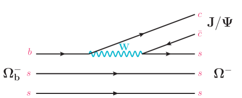
According to Fig. 1, the amplitude of $\Omega_{b}^{-}\to\Omega^{-}J/\Psi$ combines the matrix elements of the $\Omega_{b}^{-}\to\Omega^{-}$ transition and $J/\Psi$ production, written as Hsiao:2015cda ; Hsiao:2015txa

$\displaystyle{\cal M}(\Omega_{b}^{-}\to\Omega^{-}J/\Psi)$

$\displaystyle=$

$\displaystyle\frac{G_{F}}{\sqrt{2}}V_{cb}V_{cs}^{*}a_{2}\,\langle J/\psi|\bar{c}\gamma^{\mu}(1-\gamma_{5})c|0\rangle\langle\Omega^{-}|\bar{s}\gamma_{\mu}(1-\gamma_{5})b|\Omega_{b}^{-}\rangle\,,$

(2)

where $G_{F}$ is the Fermi constant, and $V_{cb(s)}^{(*)}$ the Cabibbo-Kobayashi-Maskawa (CKM) matrix element. The factorization derives that $a_{2}=c_{2}^{eff}+c_{1}^{eff}/N_{c}$, where $c_{1,2}^{eff}$ are the effective Wilson coefficients, and $N_{c}$ the color number ali ; Hsiao:2014mua . For the $J/\Psi$ production, the matrix elements read Becirevic:2013bsa

$\displaystyle\langle J/\psi|\bar{c}\gamma^{\mu}(1-\gamma_{5})c|0\rangle=m_{J/\psi}f_{J/\psi}\varepsilon_{\mu}^{*}\,,$

(3)

where $m_{J/\psi}$, $f_{J/\psi}$ and $\varepsilon_{\mu}^{*}$ are the mass, decay constant and polarization four-vector, respectively. The matrix elements of the $\Omega_{b}^{-}(bss)\to\Omega^{-}(sss)$ transition are parameterized as Zhao:2018mrg ; Gutsche:2018utw

	$\displaystyle\langle T^{\mu}\rangle\equiv\langle\Omega(sss)|\bar{s}\gamma^{\mu}(1-\gamma_{5})b|\Omega_{b}(bss)\rangle$
	$\displaystyle=\bar{u}_{\alpha}\left[\frac{P^{\alpha}}{M}\left(\gamma^{\mu}F^{V}_{1}+\frac{P^{\mu}}{M}F^{V}_{2}+\frac{P^{\,\prime\mu}}{M^{\prime}}F^{V}_{3}\right)+g^{\alpha\mu}F^{V}_{4}\right]\gamma_{5}u$
	$\displaystyle\quad-\bar{u}_{\alpha}\left[\frac{P^{\alpha}}{M}\left(\gamma^{\mu}F^{A}_{1}+\frac{P^{\mu}}{M}F^{A}_{2}+\frac{P^{\,\prime\mu}}{M^{\prime}}F^{A}_{3}\right)+g^{\alpha\mu}F^{A}_{4}\right]u\,,$		(4)

where $M^{(\prime)}$ and $P^{(\prime)}$ represent the mass and momentum of $\Omega_{b}(\Omega)$, respectively, and $F^{V,A}_{i}$ ($i=1,2,..,4$) are the form factors. By substituting the matrix elements of Eqs. (3, II) for those of Eq. (2), we derive the amplitude in the helicity basis Gutsche:2018utw ,

$\displaystyle{\cal M}$

$\displaystyle=$

$\displaystyle c_{W}\sum_{\lambda_{\Omega},\lambda_{J}}(H^{V}_{\lambda_{\Omega}\lambda_{J}}-H^{A}_{\lambda_{\Omega}\lambda_{J}})\,,$

(5)

where $c_{W}\equiv(G_{F}/\sqrt{2})V_{cb}V_{cs}^{*}\,a_{2}m_{J/\psi}f_{J/\psi}$, and $\lambda_{\Omega}=(\pm 3/2,\pm 1/2)$ and $\lambda_{J}=(0,\pm 1)$ denote the helicity states of $\Omega$ and $J/\Psi$, respectively. Due to the helicity conservation, $\lambda_{\Omega_{b}}=\lambda_{\Omega}-\lambda_{J}$ should be respected, where $\lambda_{\Omega_{b}}=\pm 1/2$. Subsequently, we obtain Gutsche:2018utw

	$\displaystyle H_{\frac{1}{2}0}^{V(A)}=\sqrt{\frac{2}{3}\frac{Q^{2}_{\mp}}{q^{2}}}\left[F_{1}^{V(A)}\left(\frac{Q^{2}_{\pm}M_{\mp}}{2MM^{\prime}}\right)\mp\left(F_{2}^{V(A)}+F_{3}^{V(A)}\frac{M}{M^{\prime}}\right)\left(\frac{|\vec{P}^{\prime}|^{2}}{M^{\prime}}\right)\mp F_{4}^{V(A)}\bar{M}^{\prime}_{-}\right]\,,$
	$\displaystyle H_{\frac{1}{2}1}^{V(A)}=-\sqrt{\frac{Q^{2}_{\mp}}{3}}\left[F_{1}^{V(A)}\left(\frac{Q^{2}_{\pm}}{MM^{\prime}}\right)-F_{4}^{V(A)}\right]\,,$
	$\displaystyle H_{\frac{3}{2}1}^{V(A)}=\mp\sqrt{Q^{2}_{\mp}}\,F_{4}^{V(A)}\,,$		(6)

and $H^{V(A)}_{-\lambda_{\Omega}-\lambda_{J}}=\mp H^{V(A)}_{\lambda_{\Omega}\lambda_{f}}$, with $M_{\pm}=M\pm M^{\prime}$, $Q^{2}_{\pm}=M_{\pm}^{2}-q^{2}$, $\bar{M}_{\pm}^{(\prime)}=(M_{+}M_{-}\pm q^{2})/(2M^{(\prime)})$ and $|\vec{P}^{\prime}|=\sqrt{Q^{2}_{+}Q^{2}_{-}}/(2M)$.

In the light-front quark model, we can calculate the form factors. To start with, we consider the baryon as a bound state that consists of three quarks $q_{1}$, $q_{2}$ and $q_{3}$, where $q_{2,3}$ are combined as a diquark, denoted by $q_{[2,3]}$. Explicitly, the baryon bound state can be written as Dosch:1988hu

			$\displaystyle|{\bf B}(P,S,S_{z})\rangle=\int\{d^{3}p_{1}\}\{d^{3}p_{2}\}$		(7)
			$\displaystyle\times 2(2\pi)^{3}\delta^{3}(\tilde{P}-\tilde{p}_{1}-\tilde{p}_{2})\sum_{\lambda_{1},\lambda_{2}}\Psi^{SS_{z}}(\tilde{p}_{1},\tilde{p}_{2},\lambda_{1},\lambda_{2})|q_{1}(p_{1},\lambda_{1})q_{[2,3]}(p_{2},\lambda_{2})\rangle\,,$

where $p_{i}$ and $\lambda_{i}$ stand for the momentum and helicity state, respectively, and $\Psi^{SS_{z}}(\tilde{p}_{1},\tilde{p}_{2},\lambda_{1},\lambda_{2})$ is the momentum-space wave function. In the light-front frame, one defines $P=(P^{-},P^{+},P_{\bot})$ with $P^{\pm}=P^{0}\pm P^{3}$ and $P_{\bot}=(P^{1},P^{2})$, and $p_{i}=(p_{i}^{-},p_{i}^{+},p_{i\bot})$ with $p_{i}^{\pm}=p_{i}^{0}\pm p_{i}^{3}$ and $p_{i\bot}=(p_{i}^{1},p_{i}^{2})$, together with $\tilde{P}=(P^{+},P_{\bot})$ and $\tilde{p}_{i}=(p_{i}^{+},p_{i\bot})$, which result in $P^{+}P^{-}=M^{2}+P_{\bot}^{2}$ and $p_{i}^{+}p_{i}^{-}={m_{i}^{2}+p_{i\bot}^{2}}$ with $(m_{1},m_{2})=(m_{q_{1}},m_{q_{2}}+m_{q_{3}})$. Moreover, $P$ and $p_{i}$ are related as $P^{+}=p^{+}_{1}+p^{+}_{2}$ and $P_{\bot}=p_{1\bot}+p_{2\bot}$, where

	$\displaystyle p^{+}_{1}=(1-x)P^{+}\,,\;p^{+}_{2}=xP^{+}\,,\;$
	$\displaystyle p_{1\bot}=(1-x)P_{\bot}-k_{\bot}\,,\;p_{2\bot}=xP_{\bot}+k_{\bot}\,,$		(8)

with $k_{\perp}$ from $\vec{k}=(k_{\perp},k_{z})$ the relative momentum. By means of $e_{i}\equiv\sqrt{m^{2}_{i}+\vec{k}^{2}}$ the energy of the (di)quark and $M_{0}\equiv e_{1}+e_{2}$, the above parameters can be rewritten as

$\displaystyle(x,1-x)=(e_{2}-k_{z},e_{1}+k_{z})/(e_{1}+e_{2})\,,\;k_{z}=\frac{xM_{0}}{2}-\frac{m^{2}_{2}+k^{2}_{\perp}}{2xM_{0}}\,.$

(9)

In addition, we obtain $M_{0}^{2}=(m_{1}^{2}+k_{\bot}^{2})/(1-x)+(m_{2}^{2}+k_{\bot}^{2})/x$. We also get $(\bar{P}_{\mu}\gamma^{\mu}-M_{0})u(\bar{P},S_{z})=0$ with $\bar{P}\equiv p_{1}+p_{2}$, where $p_{1,2}$ describe the internal motions of the internal quarks. Under the Melosh transformation Melosh:1974cu , we derive $\Psi^{SS_{z}}$ as Ke:2012wa ; Ke:2017eqo ; Zhao:2018mrg ; Hu:2020mxk

$\displaystyle\Psi^{SS_{z}}(\tilde{p}_{1},\tilde{p}_{2},\lambda_{1},\lambda_{2})$

$\displaystyle=$

$\displaystyle\sqrt{\frac{C}{2(p_{1}\cdot\bar{P}+m_{1}M_{0})}}\;\bar{u}(p_{1},\lambda_{1})\Gamma u(\bar{P},S_{z})\phi(x,k_{\perp})\,,$

(10)

where $\Gamma=\Gamma_{S}(\Gamma_{A}^{(\alpha)})$ represents the vertex function for the scalar (axial-vector) quantity of the diquark, given by Ke:2012wa ; Ke:2017eqo ; Zhao:2018mrg ; Hu:2020mxk

	$\displaystyle\Gamma_{S}=1\,,\;$
	$\displaystyle\Gamma_{A}=-\frac{1}{\sqrt{3}}\gamma_{5}\epsilon\!\!/^{*}(p_{2},\lambda_{2})\,,\;\Gamma_{A}^{\alpha}=\epsilon^{*\alpha}(p_{2},\lambda_{2})\,.$		(11)

Moreover, the parameter $C$ for $(\Gamma_{S(A)},\Gamma_{A}^{\alpha})$ is given by

$\displaystyle C=\bigg{(}\frac{3(m_{1}M_{0}+p_{1}\cdot\bar{P})}{3m_{1}M_{0}+p_{1}\cdot\bar{P}+2(p_{1}\cdot p_{2})(p_{2}\cdot\bar{P})/m_{2}^{2}}\,,\;\frac{3m_{2}^{2}M_{0}^{2}}{2m_{2}^{2}M_{0}^{2}+(p_{2}\cdot\bar{P})^{2}}\bigg{)}\,.$

(12)

In Eq. (10), $\phi(x,k_{\perp})$ is the wave function that illustrates the momentum distribution of the constituent quark-diquark states. Here, we present $\phi(x,k_{\perp})$ in the Gaussian form Hsiao:2020gtc ; Zhao:2018zcb ; Ke:2012wa ; Ke:2017eqo ; Zhao:2018mrg ; Hu:2020mxk ; Ke:2019smy :

$\displaystyle\phi(x,k_{\perp})$

$\displaystyle=$

$\displaystyle 4\left(\frac{\pi}{\beta^{2}}\right)^{3/4}\sqrt{\frac{e_{1}e_{2}}{x(1-x)M_{0}}}\exp\left(\frac{-\vec{k}^{2}}{2\beta^{2}}\right)\,,$

(13)

with $\beta\equiv\beta_{b[ss]}(\beta_{s[ss]})$ to shape the momentum distribution of the $b$-$[ss]$ ($s$-$[ss]$) system in the $\Omega_{b}$ ($\Omega$) bound state.

Using the bound states of $|\Omega_{b}(P,S,S_{z})\rangle$ and $|\Omega(P,^{\prime}S^{\prime},S^{\prime}_{z})\rangle$ in Eq. (7) and the above identities, we derive the matrix elements of the $\Omega_{b}\to\Omega$ transition in the light-front frame, given by Zhao:2018mrg

	$\displaystyle\langle\bar{T}^{\mu}\rangle$	$\displaystyle\equiv$	$\displaystyle\langle\Omega(P^{\,\prime},S^{\prime}=3/2,S_{z}^{\prime})|\bar{s}\gamma^{\mu}(1-\gamma_{5})b|\Omega_{b}(P,S=1/2,S_{z})\rangle$		(14)
		$\displaystyle=$	$\displaystyle\int\{d^{3}p_{2}\}\hat{C}^{-1/2}\phi^{\prime}(x^{\prime},k_{\perp}^{\prime})\phi(x,k_{\perp})$
			$\displaystyle\times\sum_{\lambda_{2}}\bar{u}_{\alpha}(\bar{P}^{\,\prime},S_{z}^{\,\prime})\left[\bar{\Gamma}^{\,\prime\alpha}_{A}(p\!\!/_{1}^{\prime}+m_{1}^{\prime})\gamma^{\mu}(1-\gamma_{5})(p\!\!/_{1}+m_{1})\Gamma_{A}\right]u(\bar{P},S_{z})\,,$

where $m_{1}^{(\prime)}=m_{b(s)}$, $\bar{\Gamma}=\gamma^{0}\Gamma^{\dagger}\gamma^{0}$ and $\hat{C}=4p_{1}^{+}p_{1}^{\prime+}(p_{1}\cdot\bar{P}+m_{1}M_{0})(p_{1}^{\prime}\cdot\bar{P}^{\,\prime}+m_{1}^{\prime}M_{0}^{\prime})$.

To determine $F_{i}^{V,A}$, the identities $J_{(5)}^{\mu}\equiv\bar{u}\Gamma^{\mu\beta}(\gamma_{5})u_{\beta}$ and $\bar{J}_{(5)}^{\mu}\equiv\bar{u}\bar{\Gamma}^{\mu\beta}(\gamma_{5})u_{\beta}$ can be useful, where $\Gamma^{\mu\beta}=(\gamma^{\mu}P^{\beta},P^{\,\prime\mu}P^{\beta},P^{\mu}P^{\beta},g^{\mu\beta})$ and $\bar{\Gamma}^{\mu\beta}=(\gamma^{\mu}\bar{P}^{\beta},\bar{P}^{\,\prime\mu}\bar{P}^{\beta},\bar{P}^{\mu}\bar{P}^{\beta},g^{\mu\beta})$. We can hence perform the following calculations Zhao:2018mrg ; Hsiao:2020gtc ,

	$\displaystyle J_{5}\cdot\langle T\rangle$	$\displaystyle=$	$\displaystyle Tr\bigg{\{}u_{\beta}\bar{u}_{\alpha}\left[\frac{P^{\alpha}}{M}\left(\gamma^{\mu}F^{V}_{1}+\frac{P^{\mu}}{M}F^{V}_{2}+\frac{P^{\,\prime\mu}}{M^{\prime}}F^{V}_{3}\right)+g^{\alpha\mu}F^{V}_{4}\right]\gamma_{5}\bar{u}{\Gamma}_{\mu}^{\beta}\gamma_{5}\bigg{\}}\,,$
	$\displaystyle\bar{J}_{5}\cdot\langle\bar{T}\rangle$	$\displaystyle=$	$\displaystyle\int\{d^{3}p_{2}\}\hat{C}^{-1/2}\phi^{\prime}(x^{\prime},k_{\perp}^{\prime})\phi(x,k_{\perp})$		(15)
		$\displaystyle\times$	$\displaystyle\sum_{\lambda_{2}}Tr\bigg{\{}u_{\beta}\bar{u}_{\alpha}\left[\bar{\Gamma}^{\,\prime\alpha}_{A}(p\!\!/_{1}^{\prime}+m_{1}^{\prime})\gamma^{\mu}(p\!\!/_{1}+m_{1})\Gamma_{A}\right]u\bar{\Gamma}_{\mu}^{\beta}\gamma_{5}\bigg{\}}\,.$

By connecting $J_{5}\cdot\langle T\rangle$ to $\bar{J}_{5}\cdot\langle\bar{T}\rangle$, that is, $J_{5}\cdot\langle T\rangle=\bar{J}_{5}\cdot\langle\bar{T}\rangle$, $F_{i}^{V}$ in $J_{5}\cdot\langle T\rangle$ can be extracted with $\bar{J}_{5}\cdot\langle\bar{T}\rangle$ in the light-front quark model, as the other extractions of the ${\bf B}_{b(c)}\to{\bf B}^{(*)}$ transition form factors Hsiao:2020gtc ; Zhao:2018zcb ; Ke:2012wa ; Ke:2017eqo ; Zhao:2018mrg ; Hu:2020mxk ; Ke:2019smy . Similarly, $J\cdot\langle T\rangle=\bar{J}\cdot\langle\bar{T}\rangle$ enables us to get $F_{i}^{A}$. We will present our results in the next section.

For the numerical analysis, the CKM matrix elements and the mass (decay constant) of the $J/\Psi$ meson state are given by pdg

	$\displaystyle(V_{cb},V_{cs})$	$\displaystyle=$	$\displaystyle(A\lambda^{2},1-\lambda^{2}/2)\,,$
	$\displaystyle(m_{J/\Psi},f_{J/\Psi})$	$\displaystyle=$	$\displaystyle(3.097,0.418)~{}\text{GeV}\,,$		(16)

with $\lambda=0.2265$ and $A=0.790$ in the Wolfenstein parameterization. The effective Wilson coefficients $(c^{eff}_{1},\,c^{eff}_{2})=(1.168,-0.365)$ come from Refs. ali ; Hsiao:2014mua . In the generalized version of the factorization approach, $N_{c}$ is taken as a floating number, in order that the non-factorizable effects from QCD corrections can be estimated. By adopting $N_{c}=2.15\pm 0.17$ in Hsiao:2015cda ; Hsiao:2015txa , we obtain $a_{2}=0.18^{+0.05}_{-0.04}$, which has been used to interpret ${\cal B}(\Lambda_{b}\to\Lambda J/\psi)$ and ${\cal B}(\Xi_{b}^{-}\to\Xi^{-}J/\psi)$.

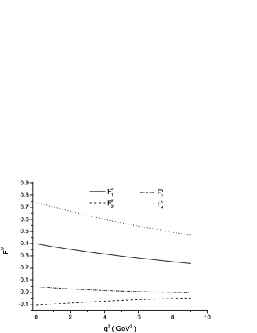
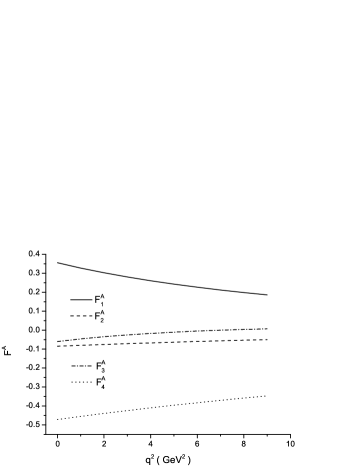
In terms of $J_{5}\cdot\langle T\rangle=\bar{J}_{5}\cdot\langle\bar{T}\rangle$ and $J\cdot\langle T\rangle=\bar{J}\cdot\langle\bar{T}\rangle$ and the theoretical inputs in Eqs. (13, 14, II), given by Ke:2019smy

	$\displaystyle(m_{b},\beta_{b[ss]})$	$\displaystyle=$	$\displaystyle(5.00\pm 0.20,0.78\pm 0.04)~{}\mathrm{GeV}\,,$
	$\displaystyle(m_{s},\beta_{s[ss]})$	$\displaystyle=$	$\displaystyle(0.38,0.48)~{}\mathrm{GeV}\,,$		(17)

we derive $F^{V(A)}_{i}$ as the functions of $q^{2}$, depicted in Fig. 2. It is common that one parameterizes the form factors in the dipole expressions Cheng:2003sm ; Choi:2013ira ; Hsiao:2019wyd , which reproduce the momentum dependences derived in the quark model. Subsequently, the form factors can have simple forms to be used in the weak decays. In our case, we present Zhao:2018zcb ; Hsiao:2020gtc

$\displaystyle F(q^{2})=\frac{F(0)}{1-a\left(q^{2}/m_{F}^{2}\right)+b\left(q^{4}/m_{F}^{4}\right)}\,,$

(18)

with $m_{F}$, $a$, $b$ and $F(0)$ at $q^{2}=0$ given in Table 1, in order to describe the momentum behaviors of $F_{i}^{V,A}$ in Fig. 2.

Thus, we calculate the branching fraction and fragmentation fraction as

	$\displaystyle{\cal B}(\Omega_{b}^{-}\to\Omega^{-}J/\Psi)=(5.3^{+3.3+3.8}_{-2.1-2.7})\times 10^{-4}\,,$
	$\displaystyle f_{\Omega_{b}}=(0.54^{+0.34+0.39+0.21}_{-0.22-0.28-0.15})\times 10^{-2}\,,$		(19)

where $f_{\Omega_{b}}$ is extracted with ${\cal B}(\Omega_{b}^{-}\to\Omega^{-}J/\Psi)$ and the data in Eq. (I). Moreover, the first and second uncertainties come from $a_{2}$ and $F_{i}^{V,A}$, respectively, and the third one for $f_{\Omega_{b}}$ is from the measurement.

Because of the insufficient information on the $\Omega_{b}\to{\bf B}^{*}$ transition, the $\Omega_{b}$ decays have not been richly explored. In the light-front quark model, we calculate the $\Omega_{b}\to\Omega$ transition form factors. We can hence predict ${\cal B}(\Omega_{b}\to\Omega J/\Psi)=(5.3^{+3.3+3.8}_{-2.1-2.7})\times 10^{-4}$, which is compatible with those of the anti-triplet $b$-baryon decays ${\cal B}(\Lambda_{b}\to\Lambda J/\Psi)=(3.3\pm 2.0)\times 10^{-4}$ and ${\cal B}(\Xi_{b}^{-}\to\Xi^{-}J/\Psi)=(5.1\pm 3.2)\times 10^{-4}$ Hsiao:2015cda ; Hsiao:2015txa . On the other hand, ${\cal B}(\Omega_{b}\to\Omega J/\Psi)=8.1\times 10^{-4}$ is given by the authors of Ref. Gutsche:2018utw . In addition, the total decay width $\Gamma(\Omega_{b}\to\Omega J/\Psi)=3.15a_{2}^{2}\times 10^{10}$ s^-1 Cheng:1996cs leads to ${\cal B}(\Omega_{b}\to\Omega J/\Psi)=16.7\times 10^{-4}$, where we have used $a_{2}=0.18$ for the demonstration.

In the helicity basis, the branching fraction is given by

$\displaystyle{\cal B}\propto(|{\cal H}_{V}|^{2}+|{\cal H}_{A}|^{2})\,,$

(20)

where $|{\cal H}_{V(A)}|^{2}\equiv|H_{\frac{3}{2}1}^{V(A)}|^{2}+|H_{\frac{1}{2}1}^{V(A)}|^{2}+|H_{\frac{1}{2}0}^{V(A)}|^{2}$. It is found that $(|{\cal H}_{V}|^{2},|{\cal H}_{A}|^{2})$ give (19,81)% of ${\cal B}$; besides, $(|H_{\frac{3}{2}1}^{A}|^{2},|H_{\frac{1}{2}1}^{A}|^{2},|H_{\frac{1}{2}0}^{A}|^{2})/|{\cal H}_{A}|^{2}=(54.0,22.4,23.6)\%$, such that $F_{4}^{A}$ gives the main contribution to ${\cal B}(\Omega_{b}\to\Omega J/\Psi)$.

In Eq. (III), $f_{\Omega_{b}}=0.54\times 10^{-2}$ agrees with the previous upper limit of 0.108 Hsiao:2015txa . By comparing our extraction to $f_{\Lambda_{b}}=0.175\pm 0.106$ and $f_{\Xi_{b}}=0.019\pm 0.013$ Hsiao:2015txa , it demonstrates that the $b$ to $\Omega_{b}$ productions are much more difficult than the $b$ to ${\bf B}_{b}$ ones. Since the fragmentation fraction has not been determined experimentally, the branching fractions of the $\Omega_{b}$ decays should be partially measured with the factor $f_{\Omega_{b}}$. Therefore, our extraction for $f_{\Omega_{b}}$ can be useful. With $f_{\Omega_{b}}$ of Eq. (III) added to the branching fractions, one can compare his theoretical results to future measurements of the $\Omega_{b}$ decays.

In summary, we have investigated the charmful $\Omega_{b}$ decay channel $\Omega_{b}^{-}\to\Omega^{-}J/\Psi$. In the light-front quark model, we have studied the $\Omega_{b}\to\Omega$ transition form factors $(F_{i}^{V},F_{i}^{A})$ ($i=1,2,...,4$). We have hence predicted ${\cal B}(\Omega_{b}^{-}\to\Omega^{-}J/\Psi)=(5.3^{+3.3+3.8}_{-2.1-2.7})\times 10^{-4}$, which is compatible with those of the $\Lambda_{b}\to\Lambda J/\Psi$ and $\Xi_{b}^{-}\to\Xi^{-}J/\Psi$ decays. In addition, $F_{4}^{A}$ has been found to give the main contribution. Particularly, we have extracted $f_{\Omega_{b}}=(0.54^{+0.34+0.39+0.21}_{-0.22-0.28-0.15})\times 10^{-2}$ from the partial observation $f_{\Omega_{b}}{\cal B}(\Omega_{b}^{-}\to\Omega^{-}J/\Psi)=(2.9^{+1.1}_{-0.8})\times 10^{-6}$. Since $f_{\Omega_{b}}$ has not been determined experimentally, by adding $f_{\Omega_{b}}$ to the branching fractions, one is allowed to compare his calculations to future observations of the $\Omega_{b}$ decays.

YKH was supported in part by National Science Foundation of China (Grants No. 11675030 and No. 12175128). CCL was supported in part by CTUST (Grant No. CTU109-P-108).

References

- (1) P.A. Zyla et al. [Particle Data Group], PTEP 2020, 083C01 (2020).
- (2) Y.K. Hsiao, P.Y. Lin, L.W. Luo and C.Q. Geng, Phys. Lett. B 751, 127 (2015).
- (3) Y.K. Hsiao, P.Y. Lin, C.C. Lih and C.Q. Geng, Phys. Rev. D 92, 114013 (2015).
- (4) H.Y. Jiang and F.S. Yu, Eur. Phys. J. C 78, 224 (2018).
- (5) Y.K. Hsiao, L. Yang, C.C. Lih and S.Y. Tsai, Eur. Phys. J. C 80, 1066 (2020).
- (6) Z.X. Zhao, Chin. Phys. C 42, 093101 (2018).
- (7) H.J. Melosh, Phys. Rev. D 9, 1095 (1974).
- (8) P.L. Chung, F. Coester and W.N. Polyzou, Phys. Lett. B 205, 545 (1988).
- (9) H.G. Dosch, M. Jamin and B. Stech, Z. Phys. C 42, 167 (1989).
- (10) W. Jaus, Phys. Rev. D 44, 2851 (1991).
- (11) F. Schlumpf, Phys. Rev. D 47, 4114 (1993); Erratum: [Phys. Rev. D 49, 6246 (1994)].
- (12) C.Q. Geng, C.C. Lih and W.M. Zhang, Mod. Phys. Lett. A 15, 2087 (2000).
- (13) C.R. Ji and C. Mitchell, Phys. Rev. D 62, 085020 (2000).
- (14) B.L.G. Bakker and C.R. Ji, Phys. Rev. D 65, 073002 (2002).
- (15) B.L.G. Bakker, H.M. Choi and C.R. Ji, Phys. Rev. D 67, 113007 (2003).
- (16) H.Y. Cheng, C.K. Chua and C.W. Hwang, Phys. Rev. D 69, 074025 (2004).
- (17) H.M. Choi and C.R. Ji, Few Body Syst. 55, 435 (2014).
- (18) C.Q. Geng and C.C. Lih, Eur. Phys. J. C 73, 2505 (2013).
- (19) H.W. Ke, X.H. Yuan, X.Q. Li, Z.T. Wei and Y.X. Zhang, Phys. Rev. D 86, 114005 (2012).
- (20) H.W. Ke, N. Hao and X.Q. Li, J. Phys. G 46, 115003 (2019).
- (21) Z.X. Zhao, Eur. Phys. J. C 78, 756 (2018).
- (22) X.H. Hu, R.H. Li and Z.P. Xing, Eur. Phys. J. C 80, 320 (2020).
- (23) H.W. Ke, N. Hao and X.Q. Li, Eur. Phys. J. C 79, 540 (2019).
- (24) Y.K. Hsiao, S.Y. Tsai, C.C. Lih and E. Rodrigues, JHEP 2004, 035 (2020).
- (25) A. Ali, G. Kramer, and C.D. Lu, Phys. Rev. D 58, 094009 (1998).
- (26) Y.K. Hsiao and C.Q. Geng, Phys. Rev. D 91, 116007 (2015).
- (27) D. Bečirević, G. Duplančić, B. Klajn, B. Melić and F. Sanfilippo, Nucl. Phys. B 883, 306 (2014).
- (28) T. Gutsche, M.A. Ivanov, J.G. Korner and V.E. Lyubovitskij, Phys. Rev. D 98, 074011 (2018).
- (29) H.Y. Cheng, Phys. Rev. D 56, 2799 (1997).