Framing Algorithmic Recourse for Anomaly Detection
Abstract.
The problem of algorithmic recourse has been explored for supervised machine learning models, to provide more interpretable, transparent and robust outcomes from decision support systems. An unexplored area is that of algorithmic recourse for anomaly detection, specifically for tabular data with only discrete feature values. Here the problem is to present a set of counterfactuals that are deemed normal by the underlying anomaly detection model so that applications can utilize this information for explanation purposes or to recommend countermeasures. We present an approach—Context preserving Algorithmic Recourse for Anomalies in Tabular data (CARAT), that is effective, scalable, and agnostic to the underlying anomaly detection model. CARAT uses a transformer based encoder-decoder model to explain an anomaly by finding features with low likelihood. Subsequently semantically coherent counterfactuals are generated by modifying the highlighted features, using the overall context of features in the anomalous instance(s). Extensive experiments help demonstrate the efficacy of CARAT.
1. Introduction
Algorithmic recourse can be defined as a a set of actions or changes that can change the outcome for a data instance with respect to a machine learning model, typically from an unfavorable outcome to a favorable one (Joshi et al., 2019). This is an important and challenging task with practical applicability in domains such as healthcare, hiring, insurance, and commerce that incorporate machine learning models into decision support systems (Prosperi et al., 2020; Karimi et al., 2020b). Algorithmic recourse is closely related to explainability, specifically counterfactual explanations that are important to improve fairness, transparency, and trust in output of machine learning (ML) models. Indeed the most cited and intuitive explanation of algorithmic recourse presents an example how to change input features of bank loan application decided by a black-box ML algorithm to obtain a favorable outcome (Karimi et al., 2021).
Although the primary focus of algorithmic recourse has been in supervised learning contexts (Mothilal et al., 2020), specifically classification based scenarios, it is also applicable in other scenarios. In this work, we address the research of how to frame algorithmic recourse for outcomes of unsupervised anomaly detection. Specifically, we seek to obtain a set of actions to modify the feature values of a data instance deemed anomalous by a black-box anomaly detection model such that it is no longer anomalous. A motivating example would be the case of a shipment transaction that is flagged as suspicious or illegal by a monitoring system employing anomaly detection, and our exploring what needs to be modified in this transaction to no longer merit that outcome. An entity such as a trading company might seek to address its future shipment patterns, by adjusting routes, products or suppliers to avoid getting flagged as potentially fraudulent – thus motivating the problem of algorithmic recourse for anomaly detection.
Algorithmic recourse for anomaly detection has some factors that differentiates it from the classification based scenario due to the underlying ML model w.r.t. which one tries to achieve a different but favorable outcome. While classification models are supervised, anomaly detection models are mostly unsupervised, and archetypes of anomalies are difficult to determine and are application scenario dependant. Prior works consider tabular data for algorithmic recourse in the context of classification (Karimi et al., 2020b; Rawal and Lakkaraju, 2020), and use comparatively simpler datasets where features are mostly real-valued. We explore the scenario where features are strictly categorical with high dimensionality (cardinality), such as found in real world data from commerce, communication and shipping (Cao et al., 2018; Datta et al., 2020). Concepts such as proximity in the context of counterfactuals are simpler to define for real-valued data. Moreover, metrics used in classification specific algorithmic recourse do not directly translate to the scenario of anomaly detection. Our key contributions in this work are:
-
(i)
A novel formulation for the unexplored problem of algorithmic recourse for unsupervised anomaly detection.
-
(ii)
A novel approach CARAT to generate counterfactuals for anomalies in tabular data with categorical features. CARAT is demonstrated to be effective, scalable and agnostic to the underlying anomaly detection model.
-
(iii)
A new set of metrics that can effectively quantify the quality of the generated counterfactuals w.r.t. multiple objectives.
-
(iv)
Empirical results on multiple real world shipment datasets along with a case study highlighting the practical utility of our approach.
2. Preliminaries
Tabular data with strictly categorical attributes can be formally represented in terms of domains and entities (Datta et al., 2020). A domain or attribute or categorical feature is defined as a set of elements sharing a common property, e.g. Port. A domain consists of a set of entities which are the set of possible values for the categorical variable, e.g. Port: { Baltimore, New York, …}. Context (Datta et al., 2020) is defined as the reference group of entities with which an entity occurs, implying an entity can be present in multiple contexts. A data instance (record) is anomalous if it contains unexpected co-occurrence among two or more of its entities (Das and Schneider, 2007; Hu et al., 2016; Datta et al., 2020).
Definition 0 (Anomalous Record).
An anomalous record is a record where certain domains have entity values that are not consistent with the remaining entity values, termed as the context, with respect to the expected data distribution.
Explanation for a model typically refers to an attempt to convey the internal state or logic of an algorithm that leads to a decision (Wachter et al., 2017). Closely related to the idea of explanations are counterfactuals. Counterfactuals are hypothetical examples that demonstrate to an user how a different and desired prediction can be obtained. Algorithmic recourse has been defined as an actionable set of changes that can be made to change the prediction of a system with respect to a data instance from an unfavourable one to a desirable one (Joshi et al., 2019). The idea is to change one or more of the feature values of the input in an feasible manner in order to produce a favorable outcome. Algorithmic recourse has been explored in the context of mostly classification problems, with a generalized binary outcome scenario. Algorithmic recourse for anomaly detection is an important yet mostly unexplored problem. In this work, the hypothetical instances that are the result of algorithmic recourse on a data instance are referred to as counterfactuals or recourse candidates. It is important to note that while counterfactual explanations provide explanations through contrasting examples, algorithmic recourse refers to the set of actions that provides the desired outcome.
While nominal points are assumed to be generated from an underlying data distribution , anomalies can be assumed to be generated from a different distribution . It can be hypothesized that an anomaly , is generated from some through some transformation function set , such that . A simplifying view of can be a process of feature value perturbation or corruption. Therefore, we can also hypothesize that there exists some arbitrary function set , such that and possibly — which is emulated through algorithmic recourse.
Definition 0 (Algorithmic Recourse for Anomaly Detection).
Algorithmic recourse for anomaly detection can be defined as a set of actionable changes on an anomalous data instance, such that it is no longer considered an anomaly with respect to the underlying anomaly detection model.
Specifically, we consider the research question that given a row of tabular data, with strictly categorical values, which is deemed anomalous by an anomaly detection model — how can we generate a set of hypothetical records such which would be deemed normal by . In this setting, without loss of generality we consider to be (i) trained using a training set which is assumed to be clean (Chen et al., 2016; Datta et al., 2020), (ii) a likelihood based model that produces real-valued scores, (iii) a queriable black box model
Problem Description 0.
Given data instance which is deemed anomalous by a given anomaly detection model , the objective is to generate a set of counterfactuals such that is not an anomaly according to .
Since in the case of unsupervised anomaly detection an application or dataset specific threshold is often used which is difficult to determine, we can relax the definition of recourse to a obtain a set of counterfactuals such that are ranked lower by in terms of anomaly score. There are multiple objectives that require optimization to obtain counterfactuals that satisfy different criterion (Karimi et al., 2020a) such as sparsity, diversity, prolixity (Keane and Smyth, 2020), proximity to the anomalous record, low cost to the end user, along with feasibility, actionability and non-discriminatory nature which depend on application scenario. Since we address a general scenario without apriori application specific knowledge, some of these problem specific objectives such as user specific cost or feasibility are not applicable. We consider the key criterion such as validity, diversity and sparsity and discuss them on evaluation metrics in Section 5.
3. Related Work
In this section, we discuss the prior literature that explores the concepts of algorithmic recourse, counterfactuals and anomaly explanation, which are relevant in this discourse.
Explainability in machine learning models has gained burgeoning research focus over the last decade due to the need for building trust and achieving transparency in decision support systems that often employ black-box models. Post-hoc explanations through feature importance has been proposed to explain prediction of classifiers. LIME (Ribeiro et al., 2016) presents an approach to obtaining explanations through locally approximating a model in the neighborhood of of a prediction of a prediction. DeepLIFT (Shrikumar et al., 2017) proposed a method to decompose the prediction of a neural network by recursively calculating the contributions by individual neurons. SHAP (Lundberg and Lee, 2017)present a unified framework that assigns each feature an additive importance measure for a particular prediction, based on Shapley Values. InterpretML (Nori et al., 2019) presents an unified framework for Ml interpretability.
There has been recent work on explaining outcome for anomaly detection models (Antwarg et al., 2021; Macha and Akoglu, 2018; Yepmo et al., 2022). ACE (Zhang et al., 2019) proposes an approach for explaining anomalies in cybersecurity datasets. While some some anomaly detection methods such as LODI (Dang et al., 2013) and LOGP (Dang et al., 2014) provide feature importance to explain anomalies by design, most methods employ a post-hoc explanation approach. DIFFI (Carletti et al., 2020) provides explanations for outputs from an Isolation Forest. Explanation through gradient based approaches have been proposed in anomaly detection based methods on neural networks (Amarasinghe et al., 2018; Nguyen et al., 2019; Kauffmann et al., 2020).
Karimi et al. (Karimi et al., 2020b) presents a comprehensive survey on algorithmic recourse. Ustun et al. (Ustun et al., 2019) introduced the notion of actionable recourse, that ensures that the counterfactuals are obtained through appropriate feature value modification. DiCE (Mothilal et al., 2020) presents an a framework for generating and evaluating a diverse set of counterfactuals based on determinantal point processes. Neural network model based approaches for generating counterfactuals have also been proposed (Pawelczyk et al., 2020; Mahajan et al., 2019; Chapman-Rounds et al., 2021). Causal reasoning has also been explored towards algorithmic recourse (Karimi et al., 2020a; Prosperi et al., 2020; Karimi et al., 2021; Crupi et al., 2021). Approaches for recourse based on heuristics, specifically using genetic algorithms have also been explored (Sharma et al., 2019; Barredo-Arrieta and Del Ser, 2020; Dandl et al., 2020). To our knowledge, only one method RCEAA (Haldar et al., 2021) has been proposed towards recourse in anomaly detection based on autoencoders with real valued inputs.
4. Algorithmic Recourse Through Modeling Context
Algorithmic recourse consists of two steps: (i) Understanding what is causing a data instance to be an anomaly, (ii) How to define a set of actions to modify the feature values in order to remedy the unfavorable outcome. We propose CARAT: Context preserving Algorithmic Recourse for Anomalies in Tabular Data that decomposes the task into these two sequential logical steps and address them. CARAT comprises of a model based approach to identify the presence of entities that causes the record to be anomalous, and an algorithm to modify those feature values in the record for recourse.
4.1. Explainer Model
Given a record or data instance with categorical features, the tuple of entities is anomalous when one or more of the entities are out-of-context with respect to the remaining entities (Das and Schneider, 2007) with unexpected co-occurrence patterns. We use a Transformer (Vaswani et al., 2017) based architecture to jointly model the context of the entities of records. Transformers have been extensively utilized in other applications on text, image and tabular data (Huang et al., 2020). A record can be considered as a sequence of entities, without a predefined ordering of domains or any semantic interpretation of the relative ordering. Transformer based architectures are appropriate for tabular data with categorical features since (i) they can handle large cardinality values for each category and are scalable (ii) can provide contextual representations of entities (iii) can model context with a prespecified ordering of domains and do not consider any relative ordering among the domains (categories). We adopt an encoder-decoder architecture, similar to language models (Devlin et al., 2019) with the objective to predict the likelihood of each entity in a given record with possible corruptions. The predicted likelihood for each entity is conditioned on the context—implicitly capturing the pair-wise and higher order co-occurrence patterns among entities.
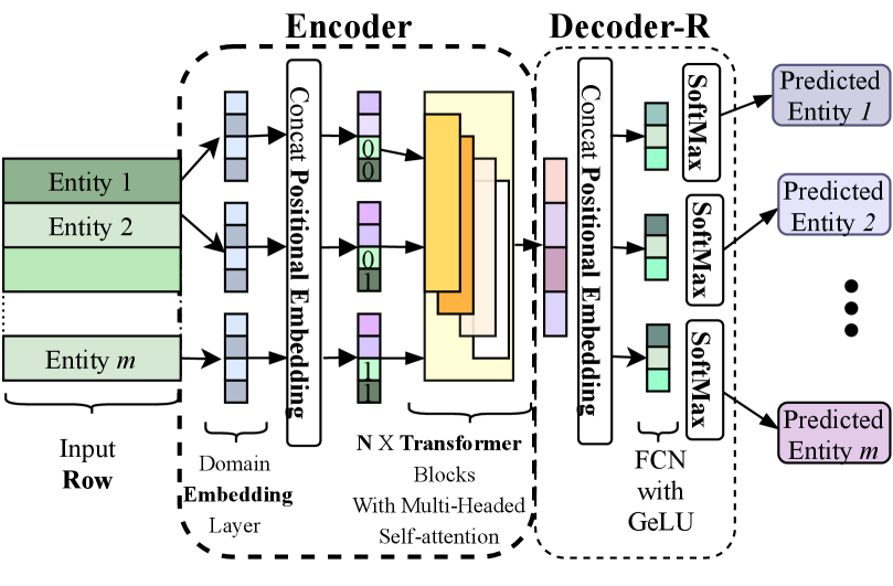
4.1.1. Pretrained Row Encoder
The encoder has a transformer based architecture and consists of multiple layers. Sequential architectures are not effective for rows of tabular data where the relative ordering of entities (and domains) do not have any semantic interpretation. To handle domains with large number of entities, a parallel domain specific embedding layers are used with same dimensionality. To inform the model which domain an entity embedding vector belongs to, we utilize positional encoding (Devlin et al., 2019) vectors which is concatenated to each of the entity embedding vectors. The tuple of vectors is then passed to the subsequent transformer block comprising of multiple layers of transformers.
To train the encoder such that it learns contextual representation for each entity in a record, we require a corresponding decoder and training objective which we design as follows. We refer to this decoder as decoder-R, which is used for pretraining the encoder and not in the final objective. Decoder-R comprises of multiple fully connected layers and is trained to reconstruct data. In order to aid the network to retain information and reconstruct it accurately, the contextual entity embeddings from the encoder layer are augmented with positional vectors through concatenation, after the first fully connected layer. Note that both the encoder and decoder-R utilize positional encoding to indicate domain and help the model reconstruct the entity for a given domain using the contextual embedding. The remainder of the decoder-R consists of parallel dense layers with GELU activation, with the last layer being softmax to obtain the index of the entity for a specific domain. Note that while the first transformation layer is shared for entity embedding of all domains, the latter layers are domain specific. The encoder and decoder-R are jointly trained, using a reconstruction based objective, similar to Masked Language Model where we randomly perturb or remove entities from records and train the model to predict the correct one from the partial context. The trained encoder captures the shallow embedding in the first layer as well as the contextual representation of entities in the record.
4.1.2. Entity Likelihood Prediction Model
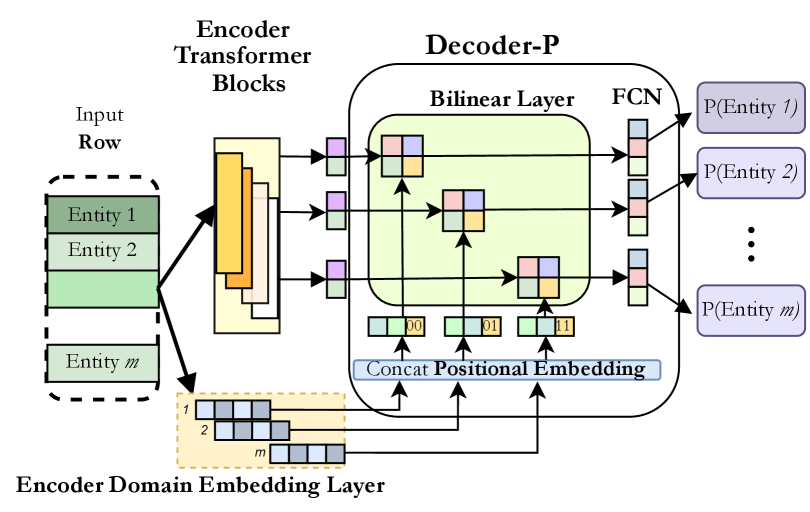
The decoder-P is designed to predict the likelihood of each entity in a record as output—using the outputs from the pretrained encoder as it’s input. The input to decoder-P consists of (i) The embedding representation for the entity , obtained from the first embedding layer of the encoder () (ii) The contextual representation of the entity , obtained from the last layer of the encoder, . Domain specific positional encoding vector () is concatenated with to obtain . We want to capture the semantic coherence and interaction between , and the contextual representation of the entity . To accomplish this we use a Bilinear layer. The output of this Bilinear layer is fed to a dense network with multiple hidden layers, and finally a sigmoid activation function to obtain a likelihood of whether an entity should occur in the given record. We utilize a simple 2-layered architecture with ReLU activation for this domain specific dense layer. Binary cross-entropy loss is used to train decoder-P, keeping the weights of the pretrained encoder fixed. The training of decoder-R differs from decoder-P due to the divergent objective. We generate labelled samples from the training data, where we perturb samples with a probability . For fraction of samples, the model is given unchanged records from the training set to enable it to recognize expected patterns and predict higher likelihood scores for co-occurring entities. For the remaining samples, we randomly perturb one or more of its entities and task the decoder to recognize which of the entities have been perturbed. It is important to note that the objective of the explainer model is not anomaly detection, but to predict the likelihoods of individual entities in a record.
4.2. Generating Counterfactuals
Records in tabular data with categorical features can be considered as tuple of entities, with data specific inherent relationships between the domains (attributes). For instance in the case of shipment records, products being shipped are closely related to the company trading them and their origin. Many real-life applications involve tabular data which can be represented as a heterogeneous graph or Heterogeneous Information Network (HIN). A HIN (Sun et al., 2011) is formally defined as a graph with a object type mapping function and edge type mapping function . Here are the nodes representing entities, are the domains, are the edges representing co-occurrence between entities and . A metapath (Sun et al., 2011) or metapath schema is an abstract path defined on the graph network schema of a heterogeneous network that describes a composite relation between nodes of type , capturing relationships between entities of different domains. There can exist multiple metapaths, and we consider and thus the metapaths to be symmetric in our problem setting. Metapaths have been utilized in similarity search in complex data, and to find patterns through capturing relevant entity relationships (Cao et al., 2018). Recent approaches on knowledge graph embeddings (KGE) (Wang et al., 2017) have demonstrated their effectiveness in capturing the semantic relationships between objects of different types in knowledge graphs which are HINs. Many approaches for KGE consider symmetric relationships as in our case, and is more generally applicable. We choose one such model DistMult (Yang et al., 2014) to obtain KGE for the entities in our data. DistMult uses both node and edge embeddings to predict semantically similar nodes, since it models relationships between entities in form of .
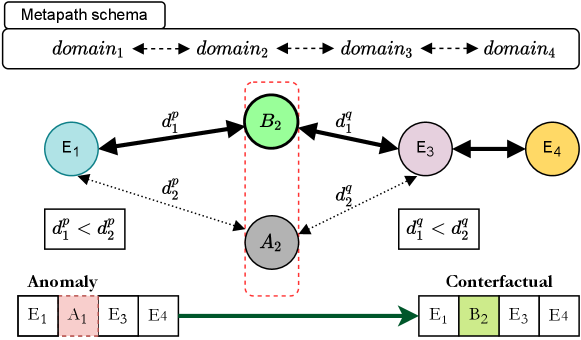
In generating counterfactuals for an anomalous record, we intend to replace the entity (or entities) which is predicted to have low likelihood by the explainer model, given the context comprising of the other entities in the record. The intuition is to replace such entities with other entities (of the corresponding domain) which are semantically similar to the other entities in the record. Let be the anomalous record and let entity in domain be selected for replacement. In this task, we utilize the associated HIN constructed from the data, along with the set of metapaths that are defined using domain knowledge. Here metapath is of the form . Thus, candidates to replace are selected using the metapaths that contain . Let us consider one such metapath such that , with relations of and . Let the respective entities in for and be and . In a generated counterfactual , the entity that replaces should ideally be semantically similar to and . KGE can be effectively used for this task. This idea is described in Figure 2. We find nearest entities to and , belonging to domain . Note that it is possible that or is null based on the schema of . We replace the entities in the domains with low likelihood with all combinations of the candidate replacements for the respective domains to obtain the set of candidate counterfactuals, of which least anomalous are chosen. The steps are summarized in Algorithm 1.
5. Evaluation Metrics
Evaluation metrics are crucial to understanding the performance of counterfactual generation methods, more so due to the fact that generated counterfactuals have multiple objectives and associated trade-offs. We discuss some of the metrics proposed in prior literature, and their limitations in the current problem setting. Further, we propose a set of new metrics that are more appropriate.
5.1. Existing Metrics for Counterfactuals
Recourse Correctness or validity (Mothilal et al., 2020) captures the ratio of counterfactuals that are accurate in terms obtaining the desired outcome from the blackbox prediction model. For unsupervised anomaly detection since provides a real valued likelihood (or anomaly score), a direct prediction (decision value) is unavailable. Recourse Coverage (Rawal and Lakkaraju, 2020) refers to quantification of the criterion that the algorithmic recourse provided covers as many instances as possible. Distance (Crupi et al., 2021; Karimi et al., 2020b) or proximity measures the mean feature-wise distance between the original data instance and the set of recourse candidates. Distance is often calculated separately for categorical and continuous attributes. For continuous attributes norms (Dhurandhar et al., 2018) or their combinations are used whereas for categorical(discrete) variables overlap measure (Chandola et al., 2007) has been used. With purely categorical attributes, this measure however fails to convey any information other than merely how many of the attributes are different in the counterfactual.
Cost (Crupi et al., 2021; Karimi et al., 2020a) refers to the cost incurred in changing a particular feature value in a recourse candidate. Prior works have utilized norms to quantify this criteria, for real-valued features. In our problem scenario, this metric is directly not applicable without any external real-world constraints which can help quantify the difference in cost in changing to vs. . Diversity (Mothilal et al., 2020) refers to the feature-wise distances between the set of recourse candidates. Diversity encourages sufficient variation among the set of recourse candidates so that it increases the chance of finding a feasible solution. However, it has been noted that in certain cases diversity as an objective correlates poorly with user cost (Yadav et al., 2021). Sparsity (Mothilal et al., 2020) refers to the number of features that are different in the recourse candidates, with respect to the original data instance.
5.2. Proposed Metrics
We propose a new set of metrics based on previously defined metrics, which are more suited to our problem setting.
Sparsity-Index: Sparsity is an important objective along with diversity that encourages minimal change is made to a data instance in terms of features. To capture this notion, we define Sparsity Index for tabular data with categorical features. Let be the anomalous record, and be the domain or feature.
| (1) |
The values of Sparsity Index , with the low value corresponding to modification of all feature values and the maximum value corresponding to none.
Coherence: We define coherence as measure to quantify the consistency of the counterfactuals similar to density consistency (Karimi et al., 2020b). Let be the set of domains which are modified in to obtain a counterfactual , be the remaining domains. Let be the entity in for domain . Coherence measures the mean probability of co-occurrence of the entities with . Maximizing coherence implies in is replaced with a candidate entity in which has a high probability of co-occurrence given the context of other entities of in , and leads to plausible counterfactuals.
| (2) |
Conditional Correctness: This metric quantifies the validity of the counterfactuals, conditional upon the underlying anomaly detection model which has a scoring function . Let be a set of randomly chosen data instances from the training and testing set. Let be the anomalous record and let the rank of in be , sorted by with appropriate order. Without loss of generalization, we can assume a higher score indicates a more normal or nominal data instance and a low score indicates anomalousness. For , where Y is the set of counterfactuals, conditional correctness can be defined as
| (3) |
This implies that is ranked lower in terms of being an anomaly, since higher ranked data instances are more anomalous. Ranking is a more suitable approach to designing a metric than utilizing thresholds which are data and application dependant an is difficult to determine. The relative ordering of records are important in this setting, since test instances are sorted based on .
Feature Accuracy: The concept of anomaly in tabular data with categorical variables has been described as one or more attributes being out of context with respect to the others, as discussed in Section 2. Therefore, it is important to accurately measure how well can a model identify which of the domain values should be modified in , and relates to the explanation aspect of algorithmic recourse. This requires having a Gold Standard (ground truth) knowledge where we know which domain values (features) have been corrupted and the entities for those domains are out of context. Let be the set of domains (features) with domains. Let be a binary valued function that has value if the domain value is changed in counterfactual from is an actual cause of the anomaly or if a domain value remains unchanged if it was not a cause of the anomaly.
| (4) |
Heterogeneity: Although diversity is an important objective for recourse candidates, existing diversity metrics like Count Diversity (Mothilal et al., 2020) are inadequate. A trivial random modification of all feature values will maximize such metrics for our setting with strictly categorical features, where distance between discrete feature values is computed using overlap measure. Two factors are important here: (i) the variation among the entities that are proposed to replace original entity in and (ii) the correct domain’s value is modified or not. We require the Gold Standard (ground truth) to determine whether the counterfactual modifies the a correct domain’s value. In our experiments, use of synthetic anomalies enables calculation of this metric. Between any two pair of recourse candidates, heterogeneity encourages dissimilarity while taking into account if both the pair of counterfactuals modify the correct domain’s value. Let be the number of domains, be the size of the set of counterfactuals , and be 1 if the correct domain has been modified.
| (5) |
| Dataset | Source | Total entity count | Domain Count | Train size |
| Dataset-1 | US Import | 6353 | 8 | 38291 |
| Dataset-2 | US import | 6151 | 8 | 35177 |
| Dataset-3 | US import | 7340 | 8 | 43495 |
| Dataset-4 | Colombia Export | 4008 | 5 | 16758 |
| Dataset-5 | Ecuador Export | 3198 | 7 | 13956 |
6. Empirical Evaluation
The key objective here is to obtain counterfactuals for for anomalies in tabular data with categorical features. We consider MEAD (Datta et al., 2020) and APE (Chen et al., 2016) as the base anomaly detection models suited to categorical tabular data. For our comparative evaluation against baselines we use MEAD. For an objective and quantifiable analysis of the performance of our approach with possible alternatives, we perform extensive experiments to capture the varied desiderata in terms of the metrics defined in Section 5.2. Further, we analyze the computational cost as well as the stability of the proposed approach.
| Dataset | Replace-m | FIMAP | RCEAA | Xformer-R | CARAT |
| Dataset-1 | |||||
| Dataset-2 | |||||
| Dataset-3 | |||||
| Dataset-4 | |||||
| Dataset-5 |
| Dataset | Replace-m | FIMAP | RCEAA | Xformer-R | CARAT |
| Dataset-1 | |||||
| Dataset-2 | |||||
| Dataset-3 | |||||
| Dataset-4 | |||||
| Dataset-5 |
| Dataset | Replace-m | FIMAP | RCEAA | Xformer-R | CARAT |
| Dataset-1 | |||||
| Dataset-2 | |||||
| Dataset-3 | |||||
| Dataset-4 | |||||
| Dataset-5 |
| Dataset | Replace-m | FIMAP | RCEAA | Xformer-R | CARAT |
| Dataset-1 | |||||
| Dataset-2 | |||||
| Dataset-3 | |||||
| Dataset-4 | |||||
| Dataset-5 |
| Dataset | Replace-m | FIMAP | RCEAA | Xformer-R | CARAT |
| Dataset-1 | |||||
| Dataset-2 | |||||
| Dataset-3 | |||||
| Dataset-4 | |||||
| Dataset-5 |
| Replace-m | FIMAP | RCEAA | Xformer-R | CARAT |
| 0.6150 | 0.2410 | 0.1657 | 0.6752 | 0.9183 |
| Sparsity Index | Conditional Corr. | Coherence | ||||
| Dataset | APE | MEAD | APE | MEAD | APE | MEAD |
| Dataset-1 | ||||||
| Dataset-2 | ||||||
| Dataset-3 | ||||||
| Dataset-4 | ||||||
| Dataset-5 | ||||||
6.1. Datasets
The datasets used in for the experimental and evaluation setup are real world proprietary datasets of shipping records obtained from Panjiva Inc (Panjiva, 2019). Specifically we use 5 datasets with no overlap, constructed from a larger corpus of records. We consider records of a time period as the training set and subsequent time as the test set. We fix the test set size to 5000. The dataset details are described in Table 1. The training set of each dataset is used to train the AD model as well as the KGE model. Since we do not have ground truth data of anomalies, we use synthetic anomalies generated from the test set of each dataset following prior work (Chen et al., 2016), and allows us to analyze the results using the ground truth knowledge of what caused the record to be an anomaly.
6.2. Competing Baseline Methods
The area of algorithmic recourse specifically for anomaly detection is unexplored, and to the best of our knowledge only one prior work RCEAA (Haldar et al., 2021) exists on this. Prior work on algorithmic recourse deals with classification scenarios and they are not directly applicable to our setting. Moreover, as previously noted, most prior work deals with real valued or mixed valued data where the cardinality of categorical variables are significantly lower. Also, most prior approaches convert discrete variables to binary vectors through one-hot encoding and treat them as real valued vectors. We choose the following baselines for comparison:
Replace-m: This approach generates an initial candidate set of all possible records by replacing the entity values in domains simultaneously, using all possible combinations. The records in this candidate set are scored by the given anomaly detection model, and top scored (least anomalous) records are considered as set of counterfactuals. We set due to computational limitations.
FIMAP (Chapman-Rounds et al., 2021): FIMAP is a model based approach for generating counterfactuals through adverserial perturbations using a perturbation network, for a classification setting with known labels. To train the proxy classifier, a set of synthetic anomalies (assigned label ) and normal instances (assigned label ). The perturbation network, which generates counterfactuals, is trained by providing synthetic anomalies and passing the perturbed data instance to the pretrained proxy classifier, to obtain the desired label ().
RCEAA (Haldar et al., 2021): RCEAA uses an optimization based objective to exactly calculate a set of counterfactuals. Since the optimization requires real valued inputs, we adopt real-value relaxation on the one-hot encoded discrete representation of and use soft-threshold approach to obtain discrete outputs.
Xformer-R: This method utilizes the explainer model to identify entities in an anomaly with low likelihood. Counterfactuals are generated by replacing the entity in the identified domains with entity values that are sampled uniformly from the domain.
6.3. Results
We present the results for the metrics discussed in Section 5.2. For conditional correctness, we sample a set of records containing both known synthetic anomalies and normal data instances. It is important to note that no single metric quantifies the different desiderata of the generated counterfactuals. Beginning with feature accuracy, which is reported in Table 2(a) we see the approaches based on Transformer based explainer (Xformer-R and CARAT) have significantly better performance compared to the others. This demonstrates that the explainer can effectively identify entities in records which do not conform to expected co-occurrence patterns. For heterogeneity, the results are presented in Table 2(b), while CARAT performs well, but FIMAP has somewhat better performance. This can be explained by the fact that counterfactuals generated by FIMAP modify most of the entity values—which violates the sparsity objective. Next we consider coherence, which that captures how semantically similar the replaced entities are to the remaining ones in the counterfactuals generated. As reported in Table 2(c), we find CARAT performs significantly better. This implies the generated counterfactuals are consistent with the underlying data distribution. Considering sparsity, FIMAP and RECEAA have significantly lower values as shown in Table 2(d), since the counterfactuals have multiple feature values modified from the given anomaly. Replace-m has a high sparsity since a single entity is modified (m=1). Xformer-R and CARAT have similar performance in terms of sparsity. Lastly, for conditional correctness reported in Table 2(e) we find Replace-m has perfect score due to performing exhaustive search for least anomalous records. CARAT shows competitive performance here, better than other baselines. Since no single metric comprehensively captures the requisite objectives that we are trying to maximize in generating counterfactuals—we summarize the model performances across all the metrics. For each approach, we first obtain the average of the values across all datasets and then normalize them. Then we perform an unweighted average across all of these normalized metrics values to find a single performance value. The results are reported in Table 2(f), which shows CARAT has a significant overall advantage.
6.4. Stability
The process of algorithmic recourse is inherently dependant on the underlying anomaly detection model which finds the anomalous data instances. Thus it is important to understand the variation in performance of our proposed approach in the context of the underlying AD model . Here is a black-box model, and assumed to perfectly capture the underlying data distribution to find data instances that are true anomalies. We choose two embedding based algorithms for tabular data with strictly categorical features as , APE (Chen et al., 2016) and MEAD (Datta et al., 2020). We apply APE and MEAD on test sets of each of the datasets, consider of the lowest scored records as anomalies, and apply CARAT with the respective AD models on the corresponding anomalies. Comparison of the applicable metrics defined in Section 5.2 for the generated counterfactuals across multiple metrics are reported in Table 3. We observe that similar performance is obtained in both cases, demonstrating the stability of our proposed approach.
6.5. Computational Cost
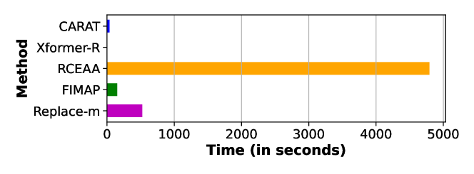
One of the major challenges of generating recourse is the computational complexity. We consider the computational cost in the execution phase, after all applicable pretraining and set up has been completed. An approach with with exponential computational complexity would be simply infeasible in most practical scenarios. For instance the Replace-m approach outlined in Section 6.2, the complexity is , where domains are chosen to be modified at most, are the cardinalities of the domains, and . RCEAA (Haldar et al., 2021) also suffers from high computational cost, as shown in Figure 3. The major bottlenecks in such an optimization based approach are: (i) expensive loss function (ii) grid search for hyperparameters (iii) operations on a very high dimensional vector due to one-hot encoding. Our proposed approach is computationally efficient, since the explanation phase uses only a pretrained model with linear time complexity and the counterfactual generation phase that requires finding nearest neighbors is sped up using an indexing library (Johnson et al., 2019).
6.6. Case Study of an Anomaly
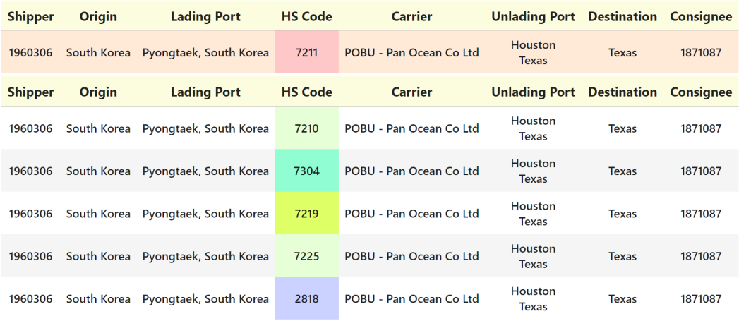
We perform a short case study based on one of the anomalies detected from test set of Dataset-1. The detected anomaly and a set of counterfactuals are shown in Figure 4. Our explainer model finds that the entity in domain HS Code in the anomalous record has low likelihood of occurrence in its context. This is supported by the empirical data, as we find goods represented by the entity HS Code:7211 was previously traded by the neither the consignee (buyer) nor the shipper. Additionally, HS Code:7211 was not previously transported through the ports of lading and unlading in the record. Our explainer only presents a low score for this entity, and not the others in the record although their context, which contains HS Code:7211, is altered. This demonstrates that the model can accurately predict likelihood from partially correct contextual information—which is the case for anomalous records. Let us look at the counterfactuals, where HS Code:7211 is modified to alternate values. HS Code:7211 refers to products of iron or non-alloy steel. Firstly HS Code:7210, HS Code:7225 and HS Code:7219 refer to products very similar to HS Code:7211, specifically rolled or non-rolled steel or alloy products. HS Code: 2818 and HS Code:7304 are metal products as well. So the counterfactuals are essentially suggesting the buyer to obtain alternate products from the supplier (shipper). This can be explained based on the data, the particular type of goods HS Code:7211 are generally not sourced from the given origin and the shipper evidenced by any similar prior occurrences. A practical explanation might relate to industrial production and proficiency patterns, since certain regions specialize in specific products. From prior records it is further observed that the consignee buys metal and alloy goods, such as with HS Codes 7210, 7323, 7304, 7225 and 7310. Thus CARAT provides meaningful counterfactuals for detected anomalies.
7. Conclusion and Future Work
In this work we address the previously unexplored problem of algorithmic recourse for anomaly detection in tabular data with categorical features with high cardinality. We propose a novel deep learning based approach CARAT to find counterfactuals for detected anomalies. We also define a set of relevant metrics that can enable effective evaluation of counterfactuals in such a problem setting. The scalability and efficacy of our model in terms of the applicable metrics as well computational cost is demonstrated through extensive experiments. However the current research leads to further research questions. While we consider multiple objectives to optimize in the process of algorithmic recourse there are application scenario specific constraints that are not considered. One of the questions that has practical implications and requires domain knowledge is the actual cost incurred by the user. Another aspect is feasibility and actionability of counterfactuals, which are often dependant on extrinsic factors that need to explicitly considered and incorporated into the algorithmic recourse for anomalies. Thus there are multiple continuing research directions which are a natural progression of the problem we address in this work.
Acknowledgements.
This work was supported in part by US NSF grants CCF-1918770, NRT DGE-1545362, and OAC-1835660 to NR, and IIS-1954376 and IIS-1815696 to FC.References
- (1)
- Amarasinghe et al. (2018) Kasun Amarasinghe, Kevin Kenney, and Milos Manic. 2018. Toward explainable deep neural network based anomaly detection. In 2018 11th ICHSI. IEEE.
- Antwarg et al. (2021) Liat Antwarg, Ronnie Mindlin Miller, Bracha Shapira, and Lior Rokach. 2021. Explaining anomalies detected by autoencoders using Shapley Additive Explanations. Expert Systems with Applications 186 (2021), 115736.
- Barredo-Arrieta and Del Ser (2020) Alejandro Barredo-Arrieta and Javier Del Ser. 2020. Plausible counterfactuals: Auditing deep learning classifiers with realistic adversarial examples. In 2020 IJCNN. IEEE.
- Cao et al. (2018) Bokai Cao et al. 2018. Collective fraud detection capturing inter-transaction dependency. In KDD 2017 Workshop on Anomaly Detection in Finance. PMLR.
- Carletti et al. (2020) Mattia Carletti, Matteo Terzi, and Gian Antonio Susto. 2020. Interpretable Anomaly Detection with DIFFI: Depth-based Isolation Forest Feature Importance. arXiv preprint arXiv:2007.11117 (2020).
- Chandola et al. (2007) Varun Chandola, Shyam Boriah, and Vipin Kumar. 2007. Similarity Measures for Categorical Data–A Comparative Study. (2007).
- Chapman-Rounds et al. (2021) Matt Chapman-Rounds et al. 2021. FIMAP: Feature Importance by Minimal Adversarial Perturbation. In AAAI, Vol. 35.
- Chen et al. (2016) Ting Chen et al. 2016. Entity embedding-based anomaly detection for heterogeneous categorical events. In IJCAI.
- Crupi et al. (2021) Riccardo Crupi et al. 2021. Counterfactual Explanations as Interventions in Latent Space. arXiv e-prints (2021), arXiv–2106.
- Dandl et al. (2020) Susanne Dandl et al. 2020. Multi-objective counterfactual explanations. In International Conference on Parallel Problem Solving from Nature. Springer, 448–469.
- Dang et al. (2013) Xuan Hong Dang et al. 2013. Local outlier detection with interpretation. In ECML PKDD. Springer, 304–320.
- Dang et al. (2014) Xuan Hong Dang et al. 2014. Discriminative features for identifying and interpreting outliers. In IEEE ICDE 2014. IEEE, 88–99.
- Das and Schneider (2007) Kaustav Das and Jeff Schneider. 2007. Detecting anomalous records in categorical datasets. In 13th ACM SIGKDD. 220–229.
- Datta et al. (2020) Debanjan Datta et al. 2020. Detecting Suspicious Timber Trades. In Proceedings of the AAAI Conference on Artificial Intelligence, Vol. 34. 13248–13254.
- Devlin et al. (2019) Jacob Devlin et al. 2019. BERT: Pre-training of Deep Bidirectional Transformers for Language Understanding. In NAACL. ACL.
- Dhurandhar et al. (2018) Amit Dhurandhar et al. 2018. Explanations based on the missing: Towards contrastive explanations with pertinent negatives. NeurIPS 31 (2018).
- Haldar et al. (2021) Swastik Haldar et al. 2021. Reliable Counterfactual Explanations for Autoencoder Based Anomalies. In 8th ACM IKDD CODS and 26th COMAD.
- Hu et al. (2016) Renjun Hu, Charu C Aggarwal, Shuai Ma, and Jinpeng Huai. 2016. An embedding approach to anomaly detection. In ICDE.
- Huang et al. (2020) Xin Huang et al. 2020. Tabtransformer: Tabular data modeling using contextual embeddings. arXiv preprint arXiv:2012.06678 (2020).
- Johnson et al. (2019) Jeff Johnson, Matthijs Douze, and Hervé Jégou. 2019. Billion-scale similarity search with gpus. IEEE Transactions on Big Data 7, 3 (2019), 535–547.
- Joshi et al. (2019) Shalmali Joshi et al. 2019. Towards realistic individual recourse and actionable explanations in black-box decision making systems. arXiv preprint arXiv:1907.09615 (2019).
- Karimi et al. (2020a) Amir-Hossein Karimi et al. 2020a. Model-agnostic counterfactual explanations for consequential decisions. In AISTATS. PMLR, 895–905.
- Karimi et al. (2020b) Amir-Hossein Karimi et al. 2020b. A survey of algorithmic recourse: definitions, formulations, solutions, and prospects. CoRR abs/2010.04050 (2020).
- Karimi et al. (2021) Amir-Hossein Karimi, Bernhard Schölkopf, and Isabel Valera. 2021. Algorithmic recourse: from counterfactual explanations to interventions. In ACM FaccT.
- Kauffmann et al. (2020) Jacob Kauffmann et al. 2020. Towards explaining anomalies: a deep Taylor decomposition of one-class models. Pattern Recognition 101 (2020), 107198.
- Keane and Smyth (2020) Mark T Keane and Barry Smyth. 2020. Good counterfactuals and where to find them: A case-based technique for generating counterfactuals for explainable AI (XAI). In International Conference on Case-Based Reasoning. Springer, 163–178.
- Lundberg and Lee (2017) Scott M Lundberg and Su-In Lee. 2017. A Unified Approach to Interpreting Model Predictions. In NeurIPS 2017, Vol. 30.
- Macha and Akoglu (2018) Meghanath Macha and Leman Akoglu. 2018. Explaining anomalies in groups with characterizing subspace rules. DMKD 2018 32 (2018).
- Mahajan et al. (2019) Divyat Mahajan et al. 2019. Preserving causal constraints in counterfactual explanations for machine learning classifiers. arXiv preprint arXiv:1912.03277 (2019).
- Mothilal et al. (2020) Ramaravind K Mothilal et al. 2020. Explaining machine learning classifiers through diverse counterfactual explanations. In ACM FAT 2020.
- Nguyen et al. (2019) Quoc Phong Nguyen et al. 2019. Gee: A gradient-based explainable variational autoencoder for network anomaly detection. In 2019 IEEE CNS. 91–99.
- Nori et al. (2019) Harsha Nori et al. 2019. Interpretml: A unified framework for machine learning interpretability. arXiv preprint arXiv:1909.09223 (2019).
- Panjiva (2019) Panjiva. 2019. Panjiva Trade Data. https://panjiva.com.
- Pawelczyk et al. (2020) Martin Pawelczyk et al. 2020. Learning model-agnostic counterfactual explanations for tabular data. In The Web Conference 2020. 3126–3132.
- Prosperi et al. (2020) Mattia Prosperi et al. 2020. Causal inference and counterfactual prediction in machine learning for actionable healthcare. NMI 2, 7 (2020).
- Rawal and Lakkaraju (2020) Kaivalya Rawal and Himabindu Lakkaraju. 2020. Beyond Individualized Recourse: Interpretable and Interactive Summaries of Actionable Recourses. NeurIPS (2020).
- Ribeiro et al. (2016) Marco Tulio Ribeiro, Sameer Singh, and Carlos Guestrin. 2016. ” Why should i trust you?” Explaining the predictions of any classifier. In 22nd ACM SIGKDD.
- Sharma et al. (2019) Shubham Sharma, Jette Henderson, and Joydeep Ghosh. 2019. Certifai: Counterfactual explanations for robustness, transparency, interpretability, and fairness of artificial intelligence models. arXiv preprint arXiv:1905.07857 (2019).
- Shrikumar et al. (2017) Avanti Shrikumar, Peyton Greenside, and Anshul Kundaje. 2017. Learning important features through propagating activation differences. In International conference on machine learning. PMLR, 3145–3153.
- Sun et al. (2011) Yizhou Sun et al. 2011. Pathsim: Meta path-based top-k similarity search in heterogeneous information networks. Proceedings of the VLDB Endowment 4, 11 (2011), 992–1003.
- Ustun et al. (2019) Berk Ustun, Alexander Spangher, and Yang Liu. 2019. Actionable recourse in linear classification. In ACM FAT. 10–19.
- Vaswani et al. (2017) Ashish Vaswani et al. 2017. Attention is all you need. In NeurIPS. 5998–6008.
- Wachter et al. (2017) Sandra Wachter et al. 2017. Counterfactual explanations without opening the black box: Automated decisions and the GDPR. Harv. JL & Tech. 31 (2017), 841.
- Wang et al. (2017) Quan Wang et al. 2017. Knowledge graph embedding: A survey of approaches and applications. IEEE TKDE 12 (2017).
- Yadav et al. (2021) Prateek Yadav et al. 2021. Low-Cost Algorithmic Recourse for Users With Uncertain Cost Functions. arXiv preprint arXiv:2111.01235 (2021).
- Yang et al. (2014) Bishan Yang et al. 2014. Embedding entities and relations for learning and inference in knowledge bases. ICLR.
- Yepmo et al. (2022) Véronne Yepmo, Grégory Smits, and Olivier Pivert. 2022. Anomaly explanation: A review. Data & Knowledge Engineering 137 (2022), 101946.
- Zhang et al. (2019) Xiao Zhang et al. 2019. ACE–an anomaly contribution explainer for cyber-security applications. In 2019 IEEE Big Data. IEEE, 1991–2000.
Appendix A Dataset Background
The datasets used in the empirical evaluation are from shipping domain and are proprietary due to security and legal reasons. We discuss some of the attributes of this real world data and their interpretations.
HS Code or Harmonized Tariff Schedule Codes are globally standardized codes that define what type of goods are being transported. Carrier is the transporting entity that operates between ports. The ports of lading and unlading are the points where the cargo is laden onto the transporting vessel or vehicle and and unladen from it. We have received help of collaborating domain experts who deal with shipping data to help us understand the data characteristics and the relationships between attributes. The original data has many attributes which contain redundant information, and we select only meaningful attributes from the raw data. Also we remove rows with missing values and perform standard data cleaning to obtain our datasets.
The metapaths that describe these relationships are shown in Table 4(c). These are designed with the knowledge of the structure of supply chains that are captured in this Bill of Lading corpus.
| Shipment Origin HS Code Port Of Lading |
| Shipment Destination HS Code Port Of Unlading |
| Port Of Lading HS Code Carrier |
| HS Code Carrier Port Of Unlading |
| Shipper Shipment Origin Port Of Lading |
| Consignee Shipment DestinationPort Of Unlading |
| Consignee Carrier Shipment Destination |
| Shipper Carrier Shipment Origin |
| Consignee Carrier Port Of Unlading |
| Shipper Carrier Port Of Lading |
| Shipper Shipment Origin HS Code |
| Consignee Shipment Destination HS Code |
| Shipment Destination HS Code Shipment Origin |
| Shipper HS Code Consignee |
| Shipment Destination,Goods Shipped,Port Of Unlading |
| Shipper Goods Shipped Shipment Origin |
| Goods Shipped Carrier Port Of Unlading |
| Consignee Shipment Destination Port Of Unlading |
| Consignee Carrier Shipment Destination |
| Shipper Carrier Shipment Origin |
| Consignee Carrier Port Of Unlading |
Appendix B Experimental Setup Details
B.1. Hardware and Libraries
We provide the implementation details to faithfully reproduce the results obtained. All implementation is done in Python 3.9, and uses standard libraries such as Numpy, Pandas and scikit-learn. For optimization and neural network based models, PyTorch (version 1.10) is used. All data preprocessing, training and evaluation presented in this work are performed on a 40-core machine, with a single GPU and distributed training required. To train our Knowledge Graph Embedding model, we use the library StellarGraph, which provides an implementation of DistMult.
B.2. Experimental Settings and Hyperparameters
B.2.1. Anomaly Detection Model
Anomaly detection for tabular data with strictly categorical features, especially where the attributes have high dimensionality (cardinality) is a challenging task. We choose Multi-relational Embedding based Anomaly Detection (Datta et al., 2020) as the base anomaly detection model for our experiments. MEAD uses an additive model based on shallow embedding, where the likelihood of a record is a function of the magnitude of transformed sum of the entity embeddings. We use an embedding size of for anomaly detection models our experiments.
B.2.2. Synthetic Anomalies
Synthetic anomalies are generated using the approach followed in prior works (Chen et al., 2016; Datta et al., 2020). For each record, randomly one or more feature values are perturbed i.e. replaced with a random but valid feature value for the categorical attribute. Since our data has at most categorical attribute we limit the number of perturbations to 2. In generating counterfactuals we consider a balanced mix for all cases.
B.2.3. CARAT Explainer Model Details
For the explainer in CARAT presented in Section 4 we an entity embedding dimension of 64. The encoder employs 4 layers of transformer blocks with 8 heads for multi-headed self-attention. The fully connected layers Decoder-R has 3 layers, with , and . The fully connected layers Decoder-P has 3 layers, with and . We use the same architecture across all datasets.
In pretraining the encoder with decoder-R, the training objective is similar to Masked Language Model but not identical. Specifically we replace approximately of entities in each records to mask, and of entities are perturbed by replacement with a randomly sample entity from the same domain. In the second phase of training the decoder-P, — the fraction of records which are not changed is set to .
Both the pre-training phase of the encoder and the final explainer architecture are trained for 250 epochs with a batch size of 512 and learning rate of . All optimization for our model and the baselines are performed using Adam.
B.2.4. CARAT KGE Details
The knowledge graph embedding model adopted here is DistMult. We use an embedding size of . The training batch size used is 1024, and we train the model for 300 epochs. We use both the node and edge embeddings to find entities that are similar to a target entity. Since DistMult uses head,rel,tail format to calculate similarity, we perform nearest neighbor search for the tail entity using precomputed embedding of head nodes and relation type.
B.3. Empirical Evaluation Setup
We generate counterfactuals for synthetic anomalies. For each approach, we use a set of 400 anomalies and we generate 50 counterfactuals for each anomaly. We use the same set of anomalies for all approaches to perform a fair comparative evaluation. For RCEAA we are able generate counterfactuals for 40 anomalies, due to the excessively long execution time as explained in Section 6.5.
B.4. Additional Detail on Competing Baselines
For the baseline models, we adapt the models to the current problem setting in an appropriate manner. We utilize the hyperparameters provided in the original work and do not perform significant hyperparameter tuning for these approaches. Similarly, we do not perform significant hyperparameter tuning for our model to tune performance as well since the objective is to demonstrate the validity of our approach in a general setting.
B.4.1. RCEAA
In our implementation of RCEAA (Haldar et al., 2021), we adapt the original approach. Firstly, we replace the autoencoder based anomaly detection model with our likelihood based model. In the loss function, we use percentile scores of training data as the threshold so that the generated counterfactuals have a low anomaly score (higher likelihood) according to our anomaly model. We set to 2. Additionally in place of euclidean distance, we use cosine distance since the dimensionality of the vectors is high. In order to reduce the computational complexity due to grid search of hyperparameters, we set the upper and lower bounds of and to and , and adopt step size of . The training epochs are increased from mentioned in the paper, to . We report the results with the lowest optimization loss.
B.4.2. FIMAP
For FIMAP, which is an approach for generating counterfactuals in a classification based setting, we adapt it to our problem setting appropriately. We adopt a more complex neural network architecture that follows that archetype proposed in the original work. Specifically, an embedding projection layer of dimensionality 32 is used for each categorical variable, whose output is concatenated and fed to a fully connected network for both proxy classifier network and perturbation network. The fully connected network for proxy classifier has size , following the original work that uses a 3 layered neural network. The fully connected network for perturbation model has size and uses dropout of . The value of in Gumbel softmax set to . We use data points to train the proxy classifier for each dataset, with samples from training set and synthetic anomalies. The batch size used is 512, and the networks are trained for 100 epochs, with early stopping.
Appendix C Code and Data Link
Please find the code for this work at :
Appendix D Ethical Implications of Algorithmic Recourse for Anomaly Detection
Since algorithmic recourse provides an approach towards generating counterfactuals that are not deemed anomalous by an anomaly detection model which may be part of a decision support system, it raises an obvious ethical question. Is algorithmic recourse adverserial to anomaly detection i.e. intended to help nefarious actors attempting to evade detection?
That is not our motivation here. First, data and anomaly detection models are expected to be secured and adverserial agents would have no access to them in order to circumvent the detection process. Recourse for anomaly detection is intended to help the decision making process. It can enable organizations like enforcement agencies in our case study, that make use of anomaly detection systems to better handle false positive cases. Verified agents, whose transactions may be erroneously flagged, could be intimated of the issue and may be provided alternatives or countermeasures. The issue of false positives exist since it is not feasible to always incorporate the application specific notions of anomaly into anomaly detection models. This effectively aids the decision support system user as well the agents whose data is being assessed. In practical scenarios, systems that utilize algorithmic recourse do require transparency and human surveillance to ensure they are used as intended. There is a minimal risk, as in any system, that unscrupulous personnel who are insiders might utilize algorithmic recourse to provide alternatives to nefarious agents enabling them avoid detection. This however can be eliminated through correct operational and access protocols where such a system is deployed.