Fringe Field Effects on Bending Magnets, Derived for TRANSPORT/TURTLE

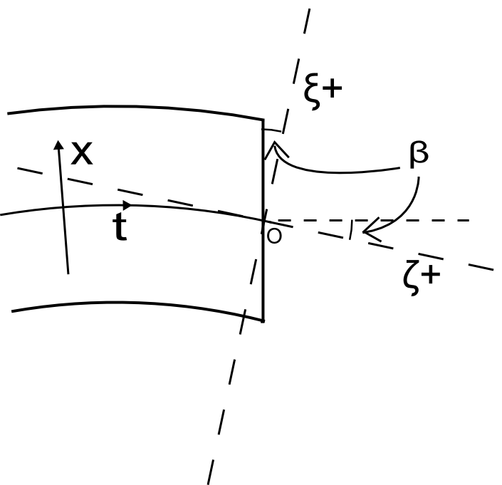
When discussing the fringe field, calculations are simplified by placing the origin of each coordinate system at the center of the pole face. The natural coordinate system defined throughout the magnet is a cylindrical curvilinear coordinate system based on the radius of curvature of the reference trajectory¹¹1The reference trajectory is the uniform trajectory of the central ray. All other rays are measured relative. given by the magnetic field within the magnet. This system is called the $(x,y,t)$ coordinate system.

A new coordinate system is introduced to describe the motion of a particle upon exiting the magnet. This coordinate system again has an origin centered on the pole face and extends rectilinearly beyond the magnet, following the reference trajectory. This coordinate system is called the $(\xi,y,\zeta)$ coordinate system. Note that the $y$ axis, in both coordinate systems, points out of the page in Fig. 2.

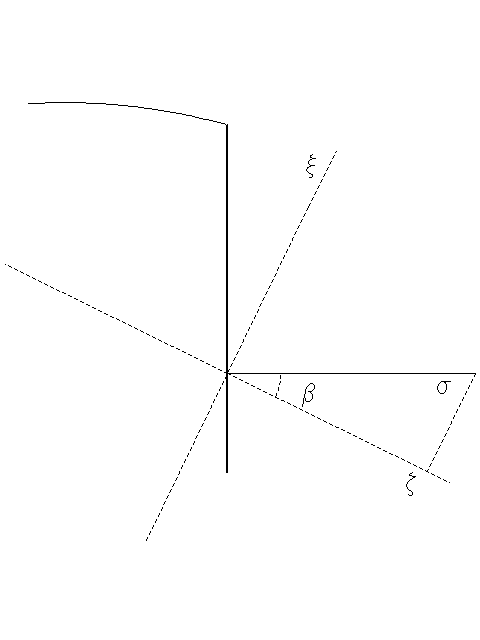
Fig. 2 depicts the new coordinate definitions based on the natural curvilinear coordinate system. In the curvilinear coordinate system, $t+$ follows the path of the reference trajectory through the magnet, and the $x$-axis points in the direction perpendicular to the $t$ axis in the bend-plane. Sometimes, a magnet’s pole face is rotated about the $y$ axis through an angle $\beta$, conventionally positive for counter-clockwise rotations when viewed from above, to modify the effects on the beam.

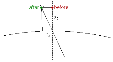
We first look to find an expression of $x$ and $t$ in terms of $\xi$ and $\zeta$ from Fig. 3. Figure 3) shows the region surrounding the pole face and a displaced particle with its corresponding position in both $(x,y,t)$ and $(\xi,y,\zeta)$. This image is centered around the origin of both coordinate systems (located at the pole face). Note that this graphic does not show the geometry of the magnet. For this reason, it should only be used for conceptualizing the relationship between coordinate systems.

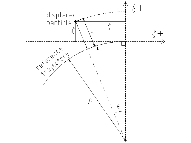
From the pythagorean theorem, we find that $(\rho+\xi)^{2}+\zeta^{2}=(\rho+x)^{2},$ or
$x=\sqrt{\zeta^{2}+(\rho+\xi)^{2}}-\rho$. To solve for $t$, we recognize that $t=\rho\theta$, where $\theta$ is the angle traversed in the path and $\rho$ is the radius of curvature. Then, $\tan\theta=\frac{\zeta}{\rho+\xi}$. Together,

		$\displaystyle x=\sqrt{\zeta^{2}+(\rho+\xi)^{2}}-\rho$
		$\displaystyle t=\rho\,\mathrm{arctan}\frac{\zeta}{\rho+\xi}.$		(1)

Solving for $\zeta$ and $\xi$, we have

	$\displaystyle\xi=\rho\left(\cos\frac{t}{\rho}-1\right)+x\cos\frac{t}{\rho}$
	$\displaystyle\zeta=(\rho+x)\sin\frac{t}{p}$		(2)

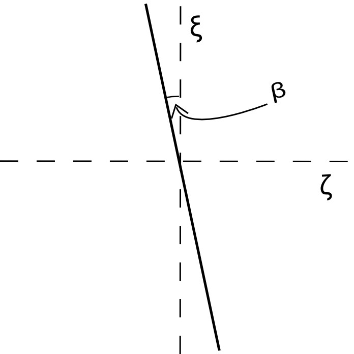
Now we construct an expression for the line that defines the exit pole-face in the $\xi\zeta$ coordinate system as seen in Fig. 4 with

$$\zeta=-\xi\tan\beta,$$

(3)

where $\beta$ is the pole-face rotation angle.

The component perpendicular to the bend plane, $y$, is identical in both coordinate systems. We retain the same coordinate name for clarity and convenience. A point in the curvilinear coordinate system is given by $(x,y,t)$ while a point in the rectilinear coordinate system is given by $(\xi,y,\zeta)$.

We begin the process of calculating the horizontal focusing effect of the fringe field. The initial position of the particle is given as $(x_{0},y_{0},0)$ in the $(x,y,t)$ coordinate system. This particle lies on the “reference plane” which is both the $xy$ plane and the $\xi y$ plane at $t=0$ and $\zeta=0$ respectively. This plane coincides with the pole face when $\beta=0$.

To calculate the horizontal effects, we must first trace the trajectory of a test particle²²2We designate an arbitrary particle off the reference trajectory as a “test particle.” It is distinct frommm the reference particle, which lies along the reference trajectory. This particle may or may not differ slightly in momentum from the reference particle. backwards in the $(x,y,t)$ coordinate system from the reference plane until it intersects the rotated pole-face. We then change to the rectilinear $(\xi,y,\zeta)$ coordinate system so that we can translate the particle through the wedge-shaped drift space. The net effect of this transformation removes the field’s effect on the particle through the region swept out by a rotation of the pole face. (Note that while this description assumes positive $\beta$ and $x_{0}$, the processes used can be rearranged for any condition. The final results are always the same.)

We know from established TRANSPORT documentation that the transformation through a dipole with radius of curvature $\rho$ and vertical magnetic field derivative $n$ (a unitless value equal to zero in the case of any relevant dipole magnet) is given as

	$\displaystyle x=x_{0}c_{x}(t)+x^{\prime}_{0}s_{x}(t)+\delta d_{x}(t)$
	$\displaystyle x^{\prime}=x_{0}c^{\prime}_{x}(t)+x^{\prime}_{0}s^{\prime}_{x}(t)+\delta d^{\prime}_{x}(t)$

where $c_{x}(t)=\cos(k_{x}t)$, $s_{x}(t)=\frac{1}{k_{x}}\sin(k_{x}t)$,
$d_{x}(t)=\frac{1}{k_{x}^{2}\rho}(1-\cos(k_{x}t))$, and $k_{x}^{2}=\frac{1-n}{\rho^{2}}$. Note that the prime indicates differentiation with respect to the longitudinal axis—in this case, $t$—for the remainder of this document. Expanding the trajectories about $t=0$, we have

	$\displaystyle x(t)$	$\displaystyle=x_{0}\left(1-\frac{k_{x}^{2}t^{2}}{2}+\dots\right)+\frac{x_{0}^{\prime}}{k_{x}}\left(k_{x}t-\frac{k_{x}^{3}t^{3}}{6}+\dots\right)$
		$\displaystyle+\frac{\delta}{k_{x}^{2}\rho}\left(1-1+\frac{k_{x}^{2}t^{2}}{2}-\dots\right)$		(4)

	$\displaystyle x^{\prime}(t)$	$\displaystyle=-x_{0}k_{x}\left(k_{x}t-\frac{k_{x}^{3}t^{3}}{6}+\dots\right)+x_{0}^{\prime}\left(1-\frac{k_{x}^{2}t^{2}}{2}+\dots\right)$
		$\displaystyle+\frac{\delta}{k_{x}\rho}\left(k_{x}t-\frac{k_{x}^{3}t^{3}}{6}+\dots\right).$		(5)

Note: We define $\delta$ as the percentage difference between the test particle’s momentum and the reference momentum.

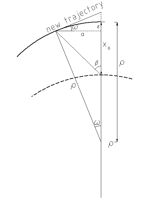
In order to transform the particle backwards through the magnetic field (described above), we evaluate $x(t_{0})$, $x^{\prime}(t_{0})$, where $t_{0}$ is the traversed longitudinal displacement from the reference plane to the pole face (see Fig. 5). Applying geometery and $x_{0}/\rho\ll 1$ from Approximation 1, we observe that $t_{0}/\rho\ll 1$. We can therefore treat it as a small quantity as we do with $x_{0}/\rho$. In fact, dividing both sides of Eq. (2.2) by $\rho$, we recognize there are several terms that contain a product of $t_{0}/\rho$ and some quantity mentioned in Approximation 1. Eliminating those terms and again multiplying through by $\rho$, we have $x=x_{0}$. Applying the same argument to Eq. (2.2), we eliminate the products of small terms, yielding $x^{\prime}=x_{0}^{\prime}$. Together,

	$\displaystyle x$	$\displaystyle=x_{0}$
	$\displaystyle x^{\prime}$	$\displaystyle=x_{0}^{\prime}.$		(6)

The above calculations show that tracing the particle backwards from the reference plane to the pole-face yields no first order changes.

The rotated pole-face geometrically yields a focusing or defocusing effect on horizontally displaced particles. Physically, the focusing effect is simply the result of passing through less (or more) field region. If a particle has a positive $x$ coordinate and the pole-face rotation angle $\beta$ is positive, then it will experience less field than the reference trajectory; likewise, if a particle has a negative $x$ coordinate and $\beta$ is positive, it will experience more field than the reference trajectory. The reverse occurs for a negative $\beta$. Thus, we can expect that a positive $\beta$ results in a defocusing effect (the horizontal exit slope of particles with negative $x_{0}$ decreases and the horizontal exit slope of particles with positive $x_{0}$ increases) and similarly a negative $\beta$ results in a focusing effect.

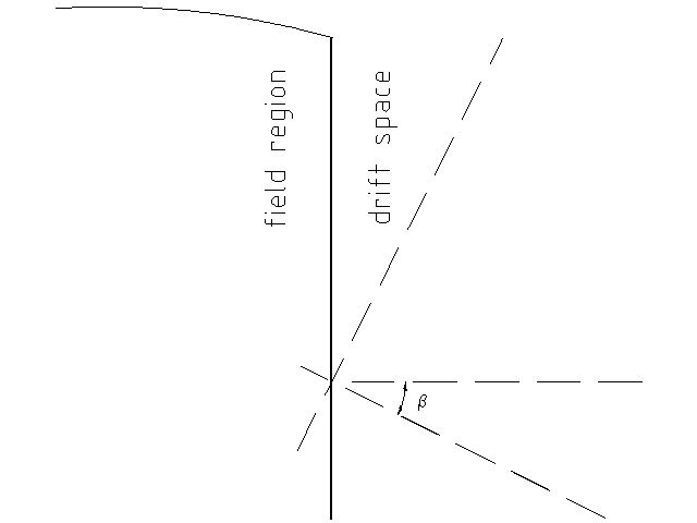
To express this behavior mathematically, we must change to the $\xi\zeta$ coordinate system to reflect the wedge-shaped, field-free region outside of the pole-face (see Fig. 6). This change in coordinate system reflects the physical fact that the particle’s direction does not change after exiting the field region: any ray will travel in a straight line once in the rectilinear coordinate system.

By Eq. (2), we recognize that when we expand $\xi$ in $t$ and evaluate it at $t=t_{0}$, Approximation 1 yields $\xi=x$. Because $x=x_{0}$ to first order at the pole face (see Eq. (6)), we conclude that, at the reference plane in the $\xi\zeta$ coordinate system, $\xi=x_{0}$. Therefore, we only look for effects in $\xi^{\prime}=\frac{d\xi}{d\zeta}$ due to the change in coordinate system.

To find these effects, we begin by applying the chain rule:

$\displaystyle\frac{d\xi}{d\zeta}=\frac{\frac{d\xi}{dt}}{\frac{d\zeta}{dt}}=\frac{\frac{\partial\xi}{\partial x}\frac{dx}{dt}+\frac{\partial\xi}{\partial t}}{\frac{\partial\zeta}{\partial x}\frac{dx}{dt}+\frac{\partial\zeta}{\partial t}}.$

From Eq. (2), we substitute in the appropriate derivatives to obtain

$$\frac{d\xi}{d\zeta}=\frac{\frac{dx}{dt}\cos\frac{t}{\rho}-\left(1+\frac{x}{\rho}\right)\sin\frac{t}{\rho}}{\frac{dx}{dt}\sin\frac{t}{\rho}+\left(1+\frac{x}{\rho}\right)\cos\frac{t}{\rho}}=\frac{x_{0}^{\prime}\cos\frac{t}{\rho}-\left(1+\frac{x_{0}}{\rho}\right)\sin\frac{t}{\rho}}{x_{0}^{\prime}\sin\frac{t}{\rho}+\left(1+\frac{x_{0}}{\rho}\right)\cos\frac{t}{\rho}}.$$

To simplify, we first expand in $t$ and evaluate at $t=t_{0}$, giving

$$\frac{d\xi}{d\zeta}=\frac{x_{0}^{\prime}\left(1-\frac{t_{0}^{2}}{2\rho^{2}}+\dots\right)-\left(1+\frac{x_{0}}{\rho}\right)\left(\frac{t_{0}}{\rho}-\frac{t_{0}^{3}}{6\rho^{3}}+\dots\right)}{x_{0}^{\prime}\left(\frac{t_{0}}{\rho}-\frac{t_{0}^{3}}{6\rho^{3}}+\dots\right)+\left(1+\frac{x_{0}}{\rho}\right)\left(1-\frac{t_{0}^{2}}{2\rho^{2}}+\dots\right)}.$$

Applying Approximation 1 yields

$$\frac{d\xi}{d\zeta}=\frac{x_{0}^{\prime}-\frac{t_{0}}{\rho}}{1+\frac{x_{0}}{\rho}}.$$

Now expanding in $x_{0}/\rho$, we find that

$$\frac{d\xi}{d\zeta}=\left(x_{0}^{\prime}-\frac{t_{0}}{\rho}\right)\left(1-\frac{x_{0}}{\rho}+\frac{x_{0}^{2}}{\rho^{2}}-\dots\right).$$

and, again applying Approximation 1,

$$\frac{d\xi}{d\zeta}=x_{0}^{\prime}-\frac{t_{0}}{\rho}.$$

Again recalling Eq. (2), we recognize that $\zeta=t$ to first order and, as before, $\xi=x$. Substituting these relations into Eq. (3), we have $t=-x\tan\beta$. Finally, substituting $-x_{0}\tan\beta$ for $t_{0}$ into the above equation yields

$$\xi^{\prime}=x_{0}^{\prime}+\frac{x_{0}}{\rho}\tan\beta.$$

To translate the particle through the wedge-shaped drift space, we apply the standard drift space transformation $\xi=\xi_{0}+\xi^{\prime}\zeta_{0}$ where, to first order, $(x_{0},t_{0})\equiv(\xi_{0},\zeta_{0})$ ($\zeta_{0}$ is the distance from the pole face to the reference plane in the $\zeta$ direction). Rewriting,

	$\displaystyle\xi=\xi_{0}+\xi^{\prime}\zeta_{0}$	$\displaystyle=x_{0}+\left(x_{0}^{\prime}+\frac{x_{0}}{\rho}\tan\beta\right)t_{0}$
		$\displaystyle=x_{0}+x_{0}^{\prime}t_{0}+t_{0}\frac{x_{0}}{\rho}\tan\beta.$

Noting from Fig. 5 that $\frac{t_{0}}{\rho}\ll 1$ and applying Approximation 1, we eliminate appropriate terms, yielding

$$\xi=x_{0}.$$

It is important to note that slopes do not change when traversing a drift space, so we still have

$$\xi^{\prime}=x_{0}^{\prime}+\frac{x_{0}}{\rho}\tan\beta.$$

Then, in order to conform to the standard coordinate system $(x,t)$, we rename $(\xi,\zeta)\equiv(x,t)$ once the particle reaches the reference plane (see Fig. 2). Thus we have

		$\displaystyle x=x_{0}$
		$\displaystyle x^{\prime}=x_{0}^{\prime}+\frac{x_{0}}{\rho}\tan\beta.$		(7)

This result is the complete transformation due to the fringe field in the horizontal direction. Figure 7 provides an intuitive geometric description of the transformation in the $x^{\prime}$ coordinate.

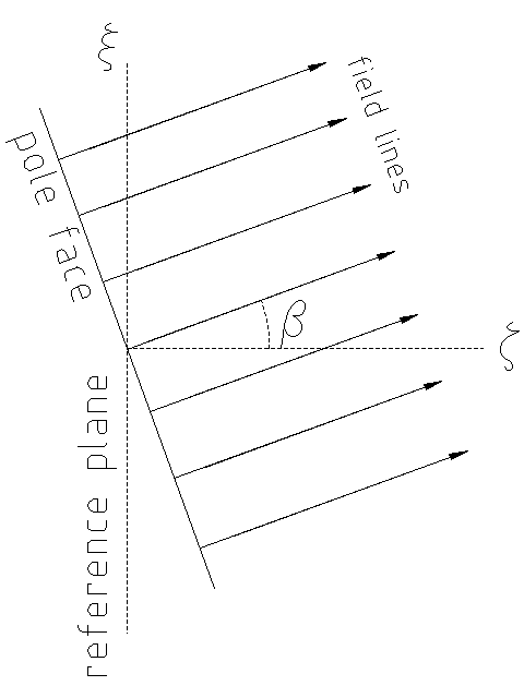
Vertical effects on rays passing through the fringe field of a dipole are caused by the element of the field perpendicular to the pole face. For the impulse approximation, if $\beta=0$, this element of the field will be in the direction of motion of the particle, causing no vertical forces on the particle and leaving the trajectory unchanged. To begin analysis, we suppose that the field $\mathbf{B}$ around the pole face also has some non-zero component in the direction perpendicular to the pole face, along with the typical field component $B_{y}$. It is important to clarify that specifics regarding the field are unnessesary for this mathematical consideration.

We begin with the trajectory coordinates before considering the effects of a vertical fringe field. Note that $y=y_{0}$ and $y^{\prime}=y_{0}^{\prime}$ before entering the fringe field.

We begin by considering the vertical component of the magnetic field in the magnet. On the interior of the magnet, the vertical component of the field has a value of $B_{0}$ and on the exterior of the magnet the vertical component of the field has a value of zero. We look to define a new axis that is perpendicular to the rotated pole-face of the magnet in order to express the field mathematically. We use the geometry of the $\xi$ and $\zeta$ axes and the pole face to construct this axis (see Fig. 9). Let us define the new axis $\sigma$ as

$$\sigma=\xi\sin\beta+\zeta\cos\beta.$$

In order to find the field components in the $\xi$ and $\zeta$ directions, we must reference one of Maxwell’s equations and see that $\nabla\times\mathbf{B}=\mathbf{0}$. That is,

$$\left|\begin{array}[]{ccc}{\hat{\xi}}&{\hat{y}}&{\hat{\zeta}}\\ \frac{\partial}{\partial\xi}&\frac{\partial}{\partial y}&\frac{\partial}{\partial\zeta}\\ B_{\xi}&B_{y}&B_{\zeta}\end{array}\right|=\mathbf{0}.$$

Hence, we have

	$\displaystyle\frac{\partial B_{\xi}}{\partial y}$	$\displaystyle=\frac{\partial B_{y}}{\partial\xi}=-B_{0}\delta(\xi\sin\beta+\zeta\cos\beta)\sin\beta$
	$\displaystyle\frac{\partial B_{\zeta}}{\partial y}$	$\displaystyle=\frac{\partial B_{y}}{\partial\zeta}=-B_{0}\delta(\xi\sin\beta+\zeta\cos\beta)\cos\beta,$

where $\delta(x)$ is the Dirac delta function.

Therefore, we can solve for $B_{\xi}$ and $B_{\zeta}$ by integrating from zero to $y_{0}$ in $y$. Because these functions are constant in $y$, this calculation is a simple process and yields, together with $B_{y}$,

	$\displaystyle B_{\xi}$	$\displaystyle=-B_{0}y_{0}\delta(\xi\sin\beta+\zeta\cos\beta)\cos\beta$
	$\displaystyle B_{y}$	$\displaystyle=B_{0}\,H(-\xi\sin\beta-\zeta\cos\beta)$
	$\displaystyle B_{\zeta}$	$\displaystyle=-B_{0}y_{0}\delta(\xi\sin\beta+\zeta\cos\beta)\sin\beta.$

As before, we write the equation of motion (see Eq. (2.3.1)) and substitute in the field components and the expression for $v_{\xi}$ (as in Eq. (11)). So, we now have

	$\displaystyle\left(y^{\prime\prime}v_{\zeta}+y^{\prime}\frac{dv_{\zeta}}{d\zeta}\right)v_{\zeta}$	$\displaystyle=\frac{q}{m}(\mathbf{v}\times\mathbf{B})_{y}$
		$\displaystyle=\frac{q}{m}(v_{\zeta}B_{\xi}-v_{\xi}B_{\zeta})$
		$\displaystyle=\frac{qB_{0}v_{\zeta}}{m}\left[\xi^{\prime}y_{0}\cos\beta-y_{0}\sin\beta\right]\,\delta(\xi\sin\beta+\zeta\cos\beta)$
	$\displaystyle y^{\prime\prime}$	$\displaystyle=\frac{1}{\rho}\left[\xi^{\prime}y_{0}\cos\beta-y_{0}\sin\beta-\frac{m}{q}y^{\prime}\frac{d}{dt}\left(\frac{d\zeta}{d\zeta}\right)\right]\,\delta(\xi\sin\beta+\zeta\cos\beta)$		(22)
	$\displaystyle y^{\prime\prime}$	$\displaystyle=\frac{1}{\rho}\left[\xi^{\prime}y_{0}\cos\beta-y_{0}\sin\beta\right]\,\delta(\xi\sin\beta+\zeta\cos\beta).$

By Approximation 1, we eliminate the second order term $\xi^{\prime}y/\rho$. We simplify the equation to

$$y^{\prime\prime}=-\frac{y_{0}}{\rho}\delta(\xi\sin\beta+\zeta\cos\beta)\sin\beta.$$

(23)

Integrating with respect to $\zeta$ across the pole-face from $-\xi\tan\beta-\epsilon$ to $-\xi\tan\beta+\epsilon$ (referencing Eq. (3)) for any $\epsilon>0$, we have

	$\displaystyle\Delta y^{\prime}$	$\displaystyle=-\frac{y_{0}\sin\beta}{\rho}\int_{-\xi\tan(\beta)-\epsilon}^{-\xi\tan(\beta)+\epsilon}\delta(\xi\sin\beta+\zeta\cos\beta)\,d\zeta$
	$\displaystyle\Delta y^{\prime}$	$\displaystyle=-\frac{y_{0}\tan\beta}{\rho}.$

This result is the total change of the slope $y^{\prime}$ from passing through the sharp cutoff field.

We then attempt to calculate the total change in the $y$ position from passing through the pole face. To do this, we take the antiderivative of both sides of Eq. (23) and integrate across the field boundary, as before, with the same bounds.

	$\displaystyle\int_{-\epsilon}^{\epsilon}\frac{dy}{d\zeta}d\zeta$	$\displaystyle=\int_{-\xi\tan(\beta)-\epsilon}^{-\xi\tan(\beta)+\epsilon}\left[-\frac{y_{0}\sin\beta}{\rho}\int\delta(\xi\sin\beta+\zeta^{*}\cos\beta)\,d\zeta^{*}\right]\,d\zeta$
	$\displaystyle\Delta y$	$\displaystyle=\int_{-\xi\tan(\beta)-\epsilon}^{-\xi\tan(\beta)+\epsilon}\left[c-\frac{y_{0}\tan\beta\,H(\xi\sin\beta+\zeta\cos\beta)}{\rho}\right]\,d\zeta$
	$\displaystyle\Delta y$	$\displaystyle=\left[c\zeta-\frac{y_{0}\tan\beta}{\rho}H(\xi\sin\beta+\zeta\cos\beta)(\zeta+\xi\sin\beta)\right]\bigg{|}_{-\xi\tan(\beta)-\epsilon}^{-\xi\tan(\beta)+\epsilon}$

We see as $\epsilon$ goes to zero,

$$\Delta y=0.$$

The above result shows that the total change of $y$ from passing through the sharp cutoff field is zero.

Thus, the transformation through the sharp cutoff field is:

	$\displaystyle y$	$\displaystyle=y_{0}$
	$\displaystyle y^{\prime}$	$\displaystyle=y_{0}^{\prime}-\frac{y_{0}\tan\beta}{\rho}.$

In this section, we look to get a better approximation than the previous impulse approximation. The impulse approximation’s sharp cutoff magnetic field cannot be physically realized. We look to find an approximation based on a finite vertical pole gap where the fringe field extends beyond that of the sharp cutoff case. Recall that the pole width is still treated as if it were infinite so that the field never has a non-zero horizontally transverse component. See Fig. 10.

We first look to define an axis perpendicular to the pole-face in the $y=0$ plane (see Fig. 9). The magnitude of the field $|\mathbf{B}|$ is then only a function of this coordinate $\sigma$ and the $y$ coordinate. That is,

$$\sigma=\frac{\zeta\cos\beta+\xi\sin\beta}{g},$$

(24)

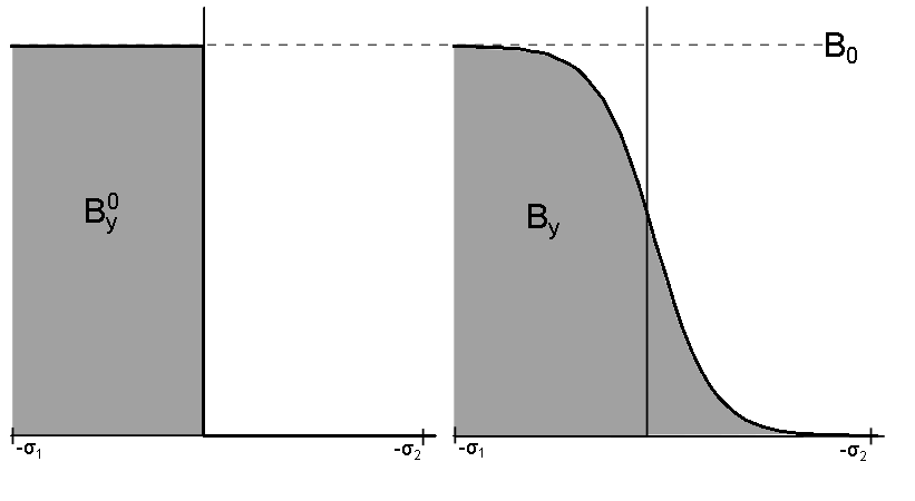
where $g$ is the vertical pole gap⁴⁴4The definition of $\sigma$ here differs from the definition given in the alternative derivation for the sharp cutoff field by a factor of $g$.. For sufficiently large positive $\sigma$, the magnitude of the field is zero. Conversely, for sufficiently large negative $\sigma$, the magnitude of the field is $B_{0}$, or the magnitude inside the magnet. We name these values $\sigma_{2}$ and $-\sigma_{1}$ respectively. Note that $\sigma_{2}$ is finite but large enough such that any remaining field is trivial.

Let $\sigma=0$ be the “effective field boundary,” or the point at which the sharp cutoff field drops to zero. Further, let $B^{0}_{y}$ be the function representing the sharp cutoff field. Consider the sharp cutoff field and the extended fringe field as functions of $\sigma$. We set the effective field boundary such that

$$\int_{-\sigma_{1}}^{\sigma_{2}}B_{y}\,d\sigma=\int_{-\sigma_{1}}^{\sigma_{2}}B_{y}^{0}\,d\sigma=\sigma_{1}B_{0},$$

(25)

where $B_{y}$ represents the magnitude of the field in the vertical direction at $y=0$ (see Fig. 11). While the definition is an approximation because $B_{y}$ does indeed vary with $y$, it is necessary and reasonable for small, practical values of $y$ (as can be seen in Fig. 10).

Finding the field components in the other two directions $\xi$ and $\zeta$ is necessary in order to apply the Lorentz force. Because $B_{y}=B_{y}(\sigma)$, we know that $B_{y}=B_{y}(\xi,\zeta)$. Applying Ampere’s Law,

$$\frac{\partial B_{\zeta}}{\partial y}=\frac{\partial B_{y}}{\partial\zeta},\,\,\,\frac{\partial B_{\xi}}{\partial y}=\frac{\partial B_{y}}{\partial\xi}.$$

Taking the antiderivative of both sides of each of the above equations with respect to $y$ yields

	$\displaystyle B_{\zeta}=\int\frac{\partial B_{y}}{\partial\zeta}dy$
	$\displaystyle B_{\xi}=\int\frac{\partial B_{y}}{\partial\xi}dy$

Evaluating the integrals on the right, we have

	$\displaystyle B_{\zeta}=y\frac{\partial B_{y}}{\partial\zeta}$
	$\displaystyle B_{\xi}=y\frac{\partial B_{y}}{\partial\xi}$

Finally, applying the chain rule from derivatives of Eq. (24),

		$\displaystyle B_{\zeta}=\frac{y\cos\beta}{g}\frac{dB_{y}}{d\sigma}$		(26)
		$\displaystyle B_{\xi}=\frac{y\sin\beta}{g}\frac{dB_{y}}{d\sigma}.$

From these expressions of the field in the three coordinate directions, we can determine the horizontal and vertical effects of the fringe field.

To calculate the horizontal trajectory, we begin with an expression of Newton’s second law in the $\xi$ direction,

	$\displaystyle m\left(\xi^{\prime\prime}v_{\zeta}+\xi^{\prime}\frac{dv_{\zeta}}{d\zeta}\right)v_{\zeta}$	$\displaystyle=q(\mathbf{v}\times\mathbf{B})_{\xi}$
		$\displaystyle=q(v_{y}B_{\zeta}-v_{\zeta}B_{y})$

From Eq. (26), we substitute in $B_{\zeta}$. Further we recognize that $v_{y}=v_{\zeta}y^{\prime}$ where the prime indicates differentiation with respect to $\zeta$ (the longitudinal axis in this coordinate system). So,

$$m\left(\xi^{\prime\prime}v_{\zeta}+\xi^{\prime}\frac{dv_{\zeta}}{d\zeta}\right)v_{\zeta}=q\left(v_{\zeta}y^{\prime}y\frac{\cos\beta}{g}\frac{dB_{y}}{d\sigma}-v_{\zeta}B_{y}\right)$$

After dividing by $mv_{\zeta}$, we use Approximation 2 and $p/q=B_{0}\rho$:

	$\displaystyle\xi^{\prime\prime}v_{\zeta}+\xi^{\prime}\frac{dv_{\zeta}}{d\zeta}$	$\displaystyle=\frac{q}{m}\left(y^{\prime}y\frac{\cos\beta}{g}\frac{dB_{y}}{d\sigma}-B_{y}\right)$
	$\displaystyle\xi^{\prime\prime}v_{\zeta}$	$\displaystyle=\frac{q}{m}\left(y^{\prime}y\frac{\cos\beta}{g}\frac{dB_{y}}{d\sigma}-B_{y}-\frac{m}{q}\xi^{\prime}\frac{d}{dt}\left[\frac{d\zeta}{d\zeta}\right]\right)$
	$\displaystyle\xi^{\prime\prime}$	$\displaystyle=\frac{1}{B_{0}\rho}\left(y^{\prime}y\frac{\cos\beta}{g}\frac{dB_{y}}{d\sigma}-B_{y}\right).$

Then, applying Approximation 1, we eliminate the term containing $y^{\prime}y/\rho$ and find

$\displaystyle\xi^{\prime\prime}=-\frac{1}{B_{0}\rho}B_{y}.$

(27)

Because $d\zeta/d\sigma=g/\cos\beta$ from Eq. (24), we multiply both sides of Eq. (27) by this quantity and apply the chain rule to both sides, yielding

$$\frac{d}{d\sigma}[\xi^{\prime}]=-\frac{g}{B_{0}\rho\cos\beta}B_{y}.$$

(28)

Integrating both sides from $-\sigma_{1}$ to $\sigma_{2}$,

$$\xi^{\prime}\big{|}_{\sigma_{2}}-\xi^{\prime}\big{|}_{-\sigma_{1}}=-\frac{g}{B_{0}\rho\cos\beta}\int_{-\sigma_{1}}^{\sigma_{2}}B_{y}d\sigma$$

(29)

We observe that Eq. (29) is valid for $B^{0}_{y}$ and $B_{y}$, the extended field case. We denote the slopes of the trajectories with subscripts $E$ and $S$ for the extended fringe field and sharp cutoff field cases respectively. Subtracting the two, we have

$$\left[\xi^{\prime}_{S}\big{|}_{\sigma_{2}}-\xi^{\prime}_{S}\big{|}_{-\sigma_{1}}\right]-\left[\xi^{\prime}_{E}\big{|}_{\sigma_{2}}-\xi^{\prime}_{E}\big{|}_{-\sigma_{1}}\right]=-\frac{g}{B_{0}\rho\cos\beta}\int_{-\sigma_{1}}^{\sigma_{2}}(B^{0}_{y}-B_{y})\,d\sigma.$$

Recognizing that the second and fourth terms on the left side both represent the slope well inside the magnet by the definition of $\sigma_{1}$, their difference is zero. Thus,

$$\xi^{\prime}_{S}\big{|}_{\sigma_{2}}-\xi^{\prime}_{E}\big{|}_{\sigma_{2}}=-\frac{g}{B_{0}\rho\cos\beta}\int_{-\sigma_{1}}^{\sigma_{2}}(B^{0}_{y}-B_{y})\,d\sigma.$$

This equation represents the difference of the slopes of the sharp cutoff case and the extended case at $\sigma_{2}$. Recalling Eq. (25),

$$\int_{-\sigma_{1}}^{\sigma_{2}}(B^{0}_{y}-B_{y})\,d\sigma=(B_{0}\sigma_{1}-B_{0}\sigma_{1})=0.$$

Then,

$$\xi^{\prime}_{S}\big{|}_{\sigma_{2}}-\xi^{\prime}_{E}\big{|}_{\sigma_{2}}=0.$$

Hence, the vertical slope of the trajectory in the bend plane in the case of the extended fringe field is equal to the slope in the sharp cutoff field. As such, $x^{\prime}=x_{0}^{\prime}+\frac{x_{0}}{\rho}\tan\beta$, just as in Eq. (2.2).

By using the process to achieve Eq. (28) twice, we find that

$$\frac{d^{2}}{d\sigma^{2}}[\xi]=-\frac{g^{2}}{B_{0}\rho\cos^{2}\beta}B_{y}.$$

We integrate twice with respect to $\sigma$ and subtract the sharp cutoff case and the extended case to find the difference in $\xi$ between the extended case and the sharp cutoff case, just as before. This process results in

	$\displaystyle\xi_{E}\big{|}_{\sigma_{2}}-\xi_{S}\big{|}_{\sigma_{2}}$	$\displaystyle=\frac{g^{2}}{B_{0}\rho\cos^{2}\beta}\int_{-\sigma_{1}}^{\sigma_{2}}\int_{-\sigma_{1}}^{\sigma^{*}}(B^{0}_{y}-B_{y})\,d\sigma\,d\sigma^{*}$
		$\displaystyle=\frac{g^{2}}{\rho\cos^{2}\beta}I_{1}$

where

$$I_{1}=\int_{-\sigma_{1}}^{\sigma_{2}}\int_{-\sigma_{1}}^{\sigma^{*}}\frac{B^{0}_{y}-B_{y}}{B_{0}}\,d\sigma\,d\sigma^{*}.$$

This difference represents the horizontal dispacement of a ray from the equivalent ray in the sharp cutoff case. This displacement affects any input ray equivalently. Therefore, the net effect is a shift in the entire beam, including the reference trajectory. Because this difference does not depend on any initial trajectory coordinates, we call this effect a “zeroth order” effect.

The final effects of the fringe field in the horizontal direction are

	$\displaystyle x=x_{0}+\frac{g^{2}}{\rho\cos^{2}\beta}I_{1}$
	$\displaystyle x^{\prime}=x_{0}^{\prime}+\frac{x_{0}}{\rho}\tan\beta.$		(30)

To adequately consider the vertical effects, we must consider the horizontal trajectory throughout the fringe field and how it affects the vertical motion. It is important to recognize that, due to the fringe field, not even the reference particle exits the magnet parallel to the $\zeta$ axis: because the fringe field is continuously decreasing to zero as opposed to a instantaneous change in the sharp cutoff case, both particles experience lesser horizontal bending effects but for longer periods of time. This phenomenon implies that particles are at an angle to the $\sigma$ axis, called $\gamma$, which continues to change until the particles are a significant distance from the pole face, at which point $\gamma(\sigma_{2})=\beta$. See Fig. 12.

Suppose a particle displaced in the $y$ direction. Because of the particle’s position along the $y$ axis, it will experience a field pointing in the $\sigma$ direction as well as the typical field in the $y$ direction while within the fringe field (see Fig. 10). The field component in the direction perpendicular to the trajectory within the bend plane is the direct cause of the vertical focusing/defocusing effects on the displaced particle. Thus, the vertical effects depend on the said field component and the speed of the particle projected into the bend plane, $v_{T}$. Let $(P,y,T)$ be a curvilinear coordinate system where the $P$ axis is always perpendicular to the particle’s trajectory $T$ in the bend plane.

References

- [1] Carey, David C. The Optics of Charged Particle Beams. Harwood Academic Publishers, 1992.
- [2] Fermilab Proposal P1021. ORKA: Measurement of the Decay at Fermilab. Fermilab, November 28, 2011.
- [3] Enge, Harald. Focusing of Charged Particles, Vol. 2. “Deflecting Magnets.”
- [4] Sagalovsk, Leonid. “Third-Order Charged Particle Beam Optics.” University of Illinois, 1989.