From Euclid to Riemann and Beyond111Dedicated to the memory of Marcel Berger (14 April 1927–15 October 2016).
– How to describe the shape of the universe –
The purpose of this essay is to trace the historical development of geometry while focusing on how we acquired mathematical tools for describing the “shape of the universe.” More specifically, our aim is to consider, without a claim to completeness, the origin of Riemannian geometry, which is indispensable to the description of the space of the universe as a “generalized curved space.”
But what is the meaning of “shape of the universe”? The reader who has never encountered such an issue might say that this is a pointless question. It is surely hard to conceive of the universe as a geometric figure such as a plane or a sphere sitting in space for which we have vocabulary to describe its shape. For instance, we usually say that a plane is “flat” and “infinite,” and a sphere is “round” and “finite.” But in what way is it possible to make use of such phrases for the universe? Behind this inescapable question is the fact that the universe is not necessarily the ordinary 3D (3-dimensional) space where the traditional synthetic geometry—based on a property of parallels which turns out to underly the “flatness” of space—is practiced. Indeed, as Einstein’s theory of general relativity (1915) claims, the universe is possibly “curved” by gravitational effects. (To be exact, we need to handle 4D curved space-times; but for simplicity we do not take the “time” into consideration, and hence treat the “static” universe or the universe at any instant of time unless otherwise stated. We shall also disregard possible “singularities” caused by “black holes.”)
An obvious problem still remains to be grappled with, however. Even if we assent to the view that the universe is a sort of geometric figure, it is impossible for us to look out over the universe all at once because we are strictly confined in it. How can we tell the shape of the universe despite that? Before Albert Einstein (1879–1955) created his theory, mathematics had already climbed such a height as to be capable to attack this issue. In this respect, Gauss and Riemann are the names we must, first and foremost, refer to as mathematicians who intensively investigated curved surfaces and spaces with the grand vision that their observations have opened up an entirely new horizon to cosmology. In particular, Riemann’s work, which completely recast three thousand years of geometry executed in “space as an a priori entity,” played an absolutely decisive role when Einstein established the theory of general relativity.
Gauss and Riemann were, of course, not the first who were involved in cosmology. Throughout history, especially from ancient Greece to Renaissance Europe, mathematicians were, more often than not, astronomers at the same time, and hence the links between mathematics and cosmology are ancient, if not in the modern sense. Meanwhile, the venerable history of cosmology (and cosmogony) overlaps in large with the history of human thought, from a reflection on primitive religious concepts to an all-embracing understanding of the world order by dint of reason. It is therefore legitimate to lead off this essay with a rough sketch of philosophical and theological aspects of cosmology in the past, while especially focusing on the image of the universe held by scientists (see Koyré [16] for a detailed account). In the course of our historical account, the reader will see how cosmology removed its religious guise through a long process of secularization and was finally established on a firm mathematical base. To be specific, Kepler, Galileo, Fermat, Descartes, Newton, Leibniz, Euler, Lagrange, and Laplace are on a short list of central figures who plowed directly or indirectly the way to the mathematization of cosmology.
The late 19th century occupies a special position in the history of mathematics. It was in this period that the autonomous progress of mathematics was getting apparent more than before. This is particularly the case after the notion of set was introduced by Cantor. His theory—in concord with the theory of topological spaces—allowed to bring in an entirely new concept of abstract space, with which one may talk not only about (in)finiteness of the universe in an intrinsic manner, an issue inherited since classical antiquity, but also about a global aspect of the universe despite that we human beings are confined to a very tiny and negligible planet in immeasurable space. In all these revolutions, Riemann’s theory (in tandem with his embryonic research of topology) became encompassed in a broader, more adequate theory, and eventually led, with a wealth of new ideas and methodology, to modern geometry.
It is not too much to say that geometry as such (and mathematics in general) is part of our cultural heritage because of the profound manifestations of the internal dynamism of human thought provoked by a “sense of wonder” (the words Aristotle used in the context of philosophy). Actually, its advances described in this essay may provide an indicator that reveals how human thought has been progressed over a long period of history.
In this essay, I do not deliberately engage myself in the cutting-edge topics of differential geometry which, combined with topology, analysis, and algebraic geometry, have been highly cultivated since the latter half of the 20th century. I also do not touch on the extrinsic study of manifolds, i.e., the theory of configurations existing in space—no doubt an equally significant theme in modern differential geometry. In this sense, the bulk of my historical commentary might be quite a bit biased towards a narrow range of geometry. The reader interested in a history of geometry (and of mathematics overall) should consult Katz [14].
Acknowledgement I wish to thank my colleague Jim Elwood whose suggestions were very helpful for the improvement of the first short draft of this essay. I am also grateful to Athanase Papadopoulos, Ken’ichi Ohshika, and Polly Wee Sy for the careful reading and for all their invaluable comments and suggestions to the enlarged version.
1 Ancient models of the universe
Since the inception of civilization that emerged in a number of far-flung places around the globe like ancient Egypt, Mesopotamia, ancient India, ancient China, and so on, mankind has struggled to understand the universe and especially how the world came to be as it is.222To know the birth and evolution of the universe is “the problem of problems” at the present day as seen in the Big Bang theory, the most prevailing hypothesis of the birth. Such attempts are seen in mythical tales about the birth of the world. “Chaos”, “water”, and the like, were thought to be the fundamental entities in its beginning that was to grow gradually into the present state. For example, the epic of Atrahasis written about 1800 BCE contains a creation myth about the Mesopotamian gods Enki (god of water), Anu (god of sky), and Enlil (god of wind). The Chinese myth in the Three Five Historic Records (the 3rd century CE) tells us that the universe in the beginning was like a big egg, inside of which was darkness chaos.333The term “chaos” (χάος) is rooted in the poem Theogony, a major source on Greek mythology, by Hesiod (ca. 750 BCE–ca. 650 BCE). The epic poet describes Chaos as the primeval emptiness of the universe.
The question of the origin is tied to the question of future. Hindu cosmology has a unique feature in this respect. In contrast to the didactics in monotheistic Christianity describing the end of the world as a single event (with the Last Judgement) in history, the Rig veda, one of the oldest extant texts in Indo-European language composed between 1500 BCE–1200 BCE, alleges that our cosmos experiences a creation-destruction cycle almost endlessly (the view celebrated much later by Nietzsche). Furthermore, some literature (e.g. the Bhagavata Purana composed between the 8th and the 10th century CE or as early as the 6th century CE) mentions the “multiverse” (infinitely many universes), which resuscitated as the modern astronomical theory of the parallel universes.
In the meantime, thinkers in colonial towns in Asia Minor, Magna Graecia, and mainland Greece, cultivated a love for systematizing phenomena on a rational basis, as opposed to supernatural explanations typified by mythology and folklore in which the cult of Olympian gods and goddesses are wrapped. Many of them were not only concerned with fundamental issues arising from everyday life, as represented by Socrates (ca. 470 BCE–399 BCE), but also labored to mathematically understand multifarious phenomena and to construct an orderly system. They appreciated purity, universality, a certainty and an elegance of mathematics, the characteristics that all other forms of knowledge do not possess. Legend has it that Plato (ca. 428 BCE–ca. 348 BCE) engraved the phrase “Let no one ignorant of geometry enter here” at the entrance of the Academeia (’Αϰαδημία) he founded in ca. 387 BCE in an outskirt of Athens. Whether or not this is historically real, Academeia indubitably put great emphasis on mathematics as a prerequisite of philosophy.444Among Plato’s thirty-five extant dialogues, there are quite a few in which the characters (Socrates in particular) discuss mathematical knowledge in one form or another; say, Hippias major, Meno, Parmenides, Theaetetus, Republic, Laws, Timaeus, Philebus. In the Republic, Book VII, Socrates says, “Geometry is fully intellectual and a study leading to the good because it deals with absolute, unchanging truths, so that it should be part of education.”
Eventually, Greek philosophers began to speculate about the structure of the universe by deploying geometric apparatus. Exemplary is the spherical model, with the earth at the center, proposed by Plato himself, and his two former students Eudoxus of Cnidus (ca. 408 BCE–ca. 355 BCE) and Aristotle from Stagira (384 BCE–322 BCE).555Pythagoras of Samos (ca. 580 BCE–ca. 500 BCE) was the first to declare that the earth is a sphere, and that the universe has a soul and intelligence. Plato was a devout Pythagorean, originally meaning the member of a mathematico-religious community created by Pythagoras (ca. 530 BCE) in Croton, Southern Italy. In his dialogue Timaeus, Plato explored cosmogonical issues, and deliberated the nature of the physical world and human beings. He referred to the demiurge (δημιουργ´ος) as the creator of the world who chose a round sphere as the most appropriate shape that embraces within itself all the shapes there are. Meanwhile, Eudoxus proposed a sophisticated system of homocentric spheres rotating about different axes through the center of the Earth, as an answer to his mentor who set the question how to reduce the apparent motions of heavenly bodies to uniform circular motions. This was stated in the treatise On velocities—now lost, but Aristotle knew about it. Eudoxus may have regarded his system simply as an abstract geometrical model; Aristotle took it to be a description of the real world, and organized it into a kind of fixed hierarchy, conjoining with his metaphysical principle (Metaphysics, XII).
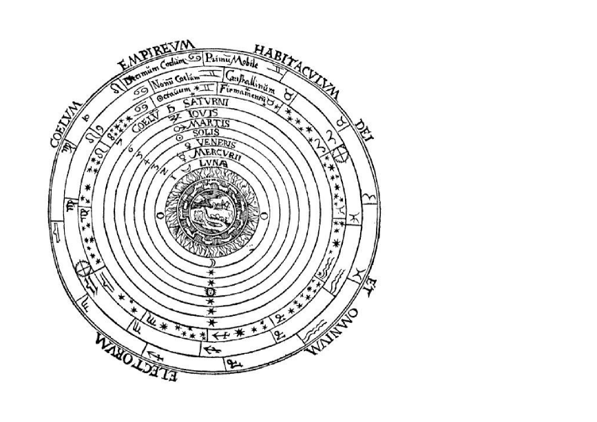
Aristotle’s spherical model (Fig. 1) was refined later as the sophisticated geocentric theory by the Alexandrian astronomer Ptolemy (ca. 100 CE–ca. 170 CE). His vision of the universe was set forth in his mathematico-astronomical treatise Almagest, and had been accepted for more than twelve hundred years in Western Europe and the Islamic world until Copernicus’ heliocentric theory emerged (Sect. 3) because his theory succeeded, up to a point, in describing the apparent motions of the sun, moon, and planets.666The title “Almagest” was derived from the Arabic name meaning “greatest.” The original Greek title is Mathematike Syntaxis (Μαϑηματιϰὴ Σ´υνταξις). It was rendered into Latin by Gerard of Cremona (ca. 1114–1187) from the Arabic version found in Toledo (1175), and became the most widely known in Western Europe before the Renaissance. What is notable in his system is the use of numerous epicycles (ἐπίϰυϰλος), where an epicycle is a small circle along which a planet is assumed to move, while each epicycle in turn moves along a larger circle (deferent).777The reasonable accuracy of Ptolemy’s system results from that an “almost periodic” motion (in the sense of H. A. Bohr)—a presumable nature of planetary motions—can be represented to any desired degree of approximation by a superposition of circular motions. This schema—a coinage of the Greek doctrine—was first set out by Apollonius of Perga (ca. 262 BCE–ca. 190 BCE), and developed further by Hipparchus of Nicaea (ca. 190 BCE–ca. 120 BCE).
At all events, an intriguing (and arguable) feature of their model is the idea of unreachable “outermost sphere.” In Aristotle’s concept (Physics, VIII, 6), it is the domain of the Prime Mover (τ`ο πρὼτη ἀϰίνητον), a variant of Plato’s notion in his cosmological argument unfolded in the Timaeus, which caused the outermost sphere to rotate at a constant angular velocity.
We shall come back to the spherical model in Sect. 3 after discussing a relevant issue, and recount at some length how this peculiar model had an effect on philosophical and religious aspects of cosmology.
2 What is infinity?
Besides the kinematical nature of celestial bodies, what seems to lie in the background of Aristotle’s view about the universe is his philosophical thought about infinity. Actually the issue of infinity was a favorite subject for Greek philosophers, dating back to the pre-Socratic period.888Anaximander of Miletus (ca. 610 BCE–ca. 546 BCE) was the first who contemplated about infinity, and employed the word apeiron (ἄπειρον meaning “unlimited”) to explain all natural phenomena in the world. Anaxagoras of Clazomenae (ca. 510 BCE–ca. 428 BCE) wrote the book About Nature, in which he says, “All things were together, infinite in number.” Assuming the infinite divisibility of matter, he avers, “There is no smallest among the small and no largest among the large, but always something still smaller and something still larger.”
Deliberating over his predecessors’ vision, Aristotle distinguished between actual and potential infinity. Briefly speaking, actual infinity is “things” that are completed and definite, thereby being transcendental in nature, while potential infinity is “things” that continue without terminating; more and more elements can be always added, but with no recognizable ending point, thus being what can be somehow corroborated within the scope of the capacity of human deed or thought. For a variety of possible reasons, Aristotle rejects actual infinity, claiming that only potential infinity exists, and captures space as something infinitely divisible into parts that are again infinitely divisible, and so on (Physics, III). His doctrine, which had satisfied nearly all scholars for a long time,999G. W. F. Hegel, a pivotal figure of German idealism, defended Aristotle’s perspective on the infinite in his Wissenschaft der Logik (1812–1816), though he used the terms “true (absolute) infinity” and “spurious infinity (schlecht Unendlichkeit)” instead. was employed by himself to find a way out of Zeno’s paradoxes, especially the paradox (παράδοξος) of Achilles and the Tortoise.101010Zeno of Elea (ca. 490 BCE–ca. 430 BCE) was a student of Parmenides (ca. 515 BCE–ca. 450 BCE) who contended that the true reality is absolutely unitary, unchanging, eternal, “the one.” To vindicate his teacher’s tenet, Zeno offered the four arguable paradoxes “The Dichotomy,” “Achilles and the Tortoise,” “The Arrow,” and “The Stadium.” During the Warring States period (476 BCE–221 BCE) in China, the School of Names cultivated a philosophy similar to Parmenides’. Hui Shi (ca. 380 BCE–ca. 305 BCE) belonging to this school says, “Ultimate greatness has no exterior, ultimate smallness has no interior.” This, in a rehashed form, says, “The fastest runner [Achilles] in a race can never overtake the slowest [tortoise], because the pursuer must first get to the point whence the pursued started, so that the slowest must always hold a lead” (Physics, VI; 9, 239b15). To quote Aristotle’s reaction in response to the quibble, Zeno’s argument exploits an ambiguity in the nature of ‘infinity’ because Zeno seems to insist that Achilles cannot complete an infinite number of his actions (getting the point where the tortoise was); that is, ‘complete’ is the word for actual infinity, but ‘infinite number of actions’ is the phrase for potential infinity.
Aristotle’s resolute rejection of actual infinity seems in part to come from the fact that mathematicians of those days had no adequate manner to treat continuous magnitude and could do, all in all, quite well without actual infinity. This is distinctively seen in the statement in Euclid’s Elements, Book IX, Prop. 20, about the infinitude of prime numbers, which deftly asserts, “Prime numbers are more than any assigned multitude of prime numbers.”111111Euclid does not seem to entirely refrain from the use of non-potential infinity. In the Elements, Book X, Def. 3, he says, “there exist straight lines infinite in multitude which are commensurable with a given one” ([7], Book X, p.10).
On the other hand, it appears that Archimedes of Syracuse (ca. 287 BCE–ca. 212 BCE) had a prescient view of infinity, as adumbrated in the Archimedes Palimpsest,121212In 1906, J. L. Heiberg, the leading authority on Archimedes, confirmed that the palimpsest, overwritten with a Christian religious text by 13th-century monks, included the Method of Mechanical Theorems, one of Archimedes’ lost works by that time. Our knowledge of Archimedes was greatly enriched by this fabulous discovery. a 10th-century Byzantine Greek copy housed at the Metochion of the Holy Sepulcher in Jerusalem. To our astonishment, in the 174-pages text (specifically in the Method, Prop. 14), he duly compared two infinite collections of certain geometric objects by means of a one-to-one correspondence (henceforth OTOC); see [21]. This is surely related to the concept of actual infinity that has been revived in 19th century (Sect. 18).
Archimedes was also a master of the method of exhaustion (or the method of double contradiction) which originated, however incomplete, with Antiphon the Sophist (ca. 480 BCE–ca. 411 BCE) and Bryson of Heraclea (born in ca. 450 BCE), and exploited by Eudoxus to avoid flaws that may happen when we treat infinity in a naive way. Such a flaw is found in the claim by the two originators; they contended that it is possible to construct, with compass and straightedge, a square with the same area as a given circle . Their argument (criticized roundly by Aristotle in the Posterior Analytics I, 9, 75b40) is as follows: From the correct fact that such a construction is possible for a given polygon (Euclid’s Elements, Book II, Prop. 14), they elicited the incorrect consequence that the same is true for on the grounds that the regular polygon with edges inscribed in eventually coincides with as we let increase endlessly (needless to say, a passage to a limit does not necessarily preserve the given properties).131313The approach taken by Antiphon and Bryson, however incorrect, was appropriately adopted by Archimedes, who obtained using two regular polygons of 96 sides inscribed and circumscribed to a circle (Measurement of the Circle).
Incidentally, the problem Antiphon and Bryson challenged is designated “squaring the circle”, one of the three big problems on constructions in Greek geometry; the other problems are “doubling the cube” and “trisecting the angle.” Anaxagoras is the first who worked on squaring the circle, while Hippocrates of Chios (ca. 470 BCE–ca. 410 BCE) squared a lune. This held out hope to square the circle for a time, but all attempts met with failure. It was in 1882 that this problem came to a conclusion; Ferdinand von Lindemann (1852–1939) proved the impossibility of such a construction by showing that is a transcendental number; i.e., is not a solution of an algebraic equation with integral coefficients (1882). Doubling the cube and trisecting the angle are also impossible as P. L. Wantzel showed (1837).
In the background of the method of exhaustion is the premise that a given quantity (not necessarily numerical) can be made smaller than another one given beforehand by successively halving . This, in modern terms, says that for any quantity , there exists a natural number with ; thus the premise goes along well with Anaxagoras’ view of “limitless smallness”141414The word “exhaustion” for this reasoning was first used by Grégoire de Saint-Vincent (1584–1667); Opus Geometricum Quadraturae Circuli et Sectionum Conti, 1647, p. 739. and is, though restricted to very special situations, regarded as a harbinger of the predicate calculus in modern logic—the branch of logic that deliberately deals with quantified statements such as “there exists an such that ” or “for any , ”— and particularly the - argument invented for the rigorous treatment of limits in the 19th century which adequately avoids endless processes (Remark 19.1). A variant of this premise is: “Given two quantities, one can find a multiple of either which will exceed the other.” This is what we call the Axiom of Archimedes since it was explicitly formulated by Archimedes in his work On the Sphere and Cylinder.151515The Elements, Book V, Def. 4 states, “Magnitudes (μέγεϑος) are said to have a ratio to one another which can, when multiplied, exceed one another.” A similar statement appears in Aristotle’s Physics VIII, 10, 266b 2. The name “Axiom of Archimedes” was given by O. Stolz in 1883, and was adopt by David Hilbert (1862–1943) in a modern treatment of Euclidean geometry (Remark 10.1 (2)). Eudoxus and Archimedes combined these premises with reductio ad absurdum (proof by contradiction) in a judicious manner,161616Reductio ad absurdum is a reasoning in the Eleatics philosophy initiated by Parmenides. Incidentally, the Chinese word for “contradiction” is “máodùn,” literally “spear-shield,” stemming from an anecdote in the Han Feizi, an ancient Chinese text attributed to the political philosopher Han Fei (ca. 280 BCE–ca. 233 BCE). The story goes as follows. A dealer of spears and shields advertised that one of his spears could pierce any shield, and at the same time said that one of his shields could defend from all spear attacks. Then one customer queried the dealer what happens when the shield and spear he mentioned would be used in a fight. and established various results on area and volume by highly sophisticated arguments. Noteworthy is that, in his computations of ratios of areas or volumes of two figures, Archimedes made use of infinitesimals in a way similar to the one in integral calculus at the early stage (e.g. Quadrature of the Parabola).
Some 1500 years later, the issue of infinity was examined by two scholars. Thomas Bradwardine (ca. 1290–ca. 1349)—a key figure in the Oxford Calculators (a group of mathematics-oriented thinkers associated with Merton College)—employed the principle of OTOC in discussing the aspects of infinite. His observation is construed, in modern terms, as “an infinite subset could be equal to its proper subset” (Tractatus de continuo, 1328–1335). This is a polemic work directed against atomistic thinkers in his time such as N. d’Autrécourt who, following the classical atomic concept, considered that matter and space were all made up of indivisible atoms, as opposed to Aristotle’s doctrine. After a while, Nicole Oresme (1320–1382), a significant scholar of the later Middle Ages, elaborated the thought that the collection of odd numbers is not smaller than that of natural numbers because it is possible to count the odd numbers by the natural numbers (Physics Commentary, around 1345).171717Oresme was in favor of the spherical model of the universe, but took a noncommittal attitude regarding the Aristotelian theory of the stationary Earth and a rotating sphere of the fixed stars (Livre du ciel et du monde and Questiones super De celo, Questiones de spera).
Meanwhile, the magic of infinity has bewildered Galileo Galilei (1564–1642). In his Discorsi e Dimostrazioni Matematiche Intorno a Due Nuove Scienze (1638), written during house arrest as the result of the Inquisition, he says, in a similar vein to Oresme’s claim, “Even though the number of squares should be less than that of all natural numbers, there appears to exist as many squares as natural numbers because any natural number corresponds to its square, and any square corresponds to its square root” (Galileo’s paradox).
Remark 2.1
(1) The principle of OTOC seems to have its roots deep in a fundamental faculty of human brain. Thinking back on how the species acquired “natural numbers” when they did not yet have any clue about numerals to count things, we are led to the speculation that they relied on the principle of OTOC. More specifically, ancient people are supposed to check whether their cattle put out to pasture returned safely to their shed, without any loss, by drawing on OTOC with some identical things such as sticks of twigs prepared in advance. They extended the same manner in counting things in various aggregations. This experience over many generations presumably made people aware that there is “something in common” behind, not depending on things, and they eventually got a way of identifying as an entity all aggregations among which there are OTOCs. This entity is nothing but a natural number.181818A. N. Whitehead said, “The first man who noticed the analogy between a group of seven fishes and a group of seven days made a notable advance in the history of thought” (Science and the Modern World, 1929).
Once reached this stage, it did not take much time for people to come up with assigning symbols and names, and evolving primitive arithmetic through empirical fumbling, especially the division algorithm, if not in the way we express it today. In fact, numerical notation systems allowing us to represent numbers with a few symbols evolved from the division algorithm. For instance, lining up rod-like symbols as is the most primitive way to represent numerals, as seen in the first few of the Babylonian and Chinese numerals. In the quinary system, we split up a given into several groups each of which consists of five rods together with a group consisting of rods less than five (this is an infantile form of the division algorithm). We then replace each by a new symbol, e.g. ; thus, for example, is exhibited as . We do the same for the symbol , and continue this procedure (this story is, of course, considerably simplified).
(2) The decimal system, contrived in India between the 1st and 4th centuries, made it possible to express every number by finitely many symbols .191919The explicit use of zero as a symbol more than a placeholder was made much later. In India, zero was initially represented by a point. The first record of the use of the symbol “0” is dated in 876 (inscribed on a stone at the Chaturbhuja Temple). The historical process leading to the term ”zero” is as follows: “sunya” in Hindu meaning emptiness “sifr” (cipher) in Arabic “zephirum” in Latin used in 1202 by Fibonacci “zero” in Italian (ca. 1600). This epochal format amplified arithmetic considerably, and was brought through the Islamic world to Europe in the 10th century. The names to be mentioned are Muhammad ibn Ms al-Khwrizmī (ca. 780 CE–ca. 850 CE), Gerbert of Aurillac (ca. 946 CE–1003), and Leonardo Fibonacci (ca. 1170 –ca 1250). In ca. 825 CE, al-Khwrizmī wrote a treatise on the decimal system. His Arabic text (now lost) was translated into Latin with the title Algoritmi de numero Indorum, most likely by Adelard of Bath (ca. 1080–ca. 1152). Gerbert is said to be the first to introduce the decimal system in Europe (probably without the numeral zero). Fibonacci, best known by the sequence with his name, travelled extensively around the Mediterranean coast, and assimilated plenty of knowledge including Islamic mathematics. His Liber Abaci (1202) popularized the decimal system in Europe.
The decimal notation—practically convenient and theoretically being of avail—is firmly planted in our brain as a mental image of numbers.
3 Is the universe infinite or finite?
Let us turn to the issue of the universe. Were Aristotle’s spherical model correct, there would be its “outside.” So the question at once arises as to what the outside means after all. Is it something substantial or just speculative fabrication? Defending this ridiculous image of the universe, Aristotle explained away by saying, “there is neither place, nor void outside the heavens by reason that the heaven does not exist inside another thing” (On the Heavens, I, 9).
Aristotle’s model continued to be employed even in the time when the Christian tenet dominated the scholarly world in Europe. Especially, influenced by Thomas Aquinas (1225–1274), who incorporated extensive Aristotelian philosophy throughout his own theology, the scientific substratum in Christianity was synthesized with the Aristotelian physics.202020In his masterwork Summa Theologiae, Aquinas asserts that God is perfect, complete, and embodies actual infinity. To reconcile his assertion with Aristotle’s doctrine, he says, “God is an infinite that has bounds.” After a while, the Florentine poet Dante Alighieri (1265–1321) reinforced Aristotle’s idea of “outside” in his unfinished work Convivio. He says, “in the supreme edifice of the universe, all the world is included, and beyond which is nothing; and it is not in space, but was formed solely in the Primal Mind.” He further offered an imaginal vision of an intriguing macrocosm in order to turn down the queer consequence of the Biblical concept of ascent to Heaven and descent to Hell which connotes that Hell is the center of the spherical universe (Sect. 21).
An exception is Nicolaus Cusanus (Nicholas of Cusa, 1401–1464), a first-class scientist of his time. He alleges, refuting the prevalent outlook of the world, “The universe is not finite in the sense of physically unboundedness since there is no special center in the universe, and hence the outermost sphere cannot be a boundary.” At the same time, he argued finiteness of the universe, by which he meant to say “privatively infinite” because “the world cannot be conceived of as finite, albeit it is not infinite” (De Docta ignorantia; 1440). This rather contradictory dictum elaborated in the ground-breaking book is a consequence of his analysis of conceivability and a parallelism between the universe and God.
A hundred years later, a dramatic turnabout took place. The heliocentric theory proposed by Nicolaus Copernicus (1473–1543) in his De revolutionibus orbium coelestium brings out the apparent retrograde motion of planets better than Ptolemy’s theory. He already got his ideas—relying largely on Arabic astronomy typified by al-Battnī212121His work Kitb az-Zīj (Book of Astronomical Tables), translated into Latin as De Motu Stellarum by Plato Tiburtinus in 1116, was quoted by Tycho Brahe, Kepler and Galileo. (ca. 858 CE–929 CE)—some time before 1541 (Commentariolus), but resisted, in spite of his friends’ persuasion, to make his theory public since he was afraid of being a target of contempt. It was in 1543, just before his death, that his work (with a preface which puts the accent on the hypothetical nature of the contents) was brought out.
Now, what did Copernicus think about the size of the universe? His model of the universe is spherical with the outermost consisting of motionless, fixed stars; thus being not much different from Aristotle’s model in this respect. Meanwhile, Giordano Bruno (1548–1600) argued against the outermost sphere (while accepting Copernicus’ theory), reasoning that the infinite power of God would not have produced a finite creation. He was quite explicit in his belief that there is no special place as the center of the universe (De l’infinito universo et mondi, 1584); thus indicating that the universe is endless, limitless, and homogeneous. His outspoken views, containing Hermetic elements, scandalized Catholics and Protestants alike.222222Some modern scholars consider him as a magus, not a pioneer of science because Hermeticism is an ancient spiritual and magical tradition. Others, however, have argued that the magical world-view in Hermeticism was a necessary precursor to the Scientific Revolution. Consequently, he was condemned as an impenitent heretic and eventually burned alive at the stake after 8 years’ solitary confinement.
Bruno’s view was partly shared by his contemporary Thomas Digges (1546–1595). He was the first to expound the Copernican system in English. In an appendix to a new edition of his father’s book A Prognostication everlasting, Digges discarded Copernicus’ notion of a fixed shell of immovable stars, presuming infinitely many stars at varying distances (1576)—a more tenable reasoning than Bruno’s. What should be thought over here is that the religious atmosphere in England in his time was different from that in the Continent because of the English Reformation that started in the reign of Henry VIII..
Interrupting the chronological account, we shall go back to ancient Greece, where we find forerunners of Cusanus, Copernicus, and Bruno. Among them, Archytas of Tarentum (428 BCE–347 BCE) is a precursor of Bruno. He inferred that any place in our space looks the same, and hence no boundary can exist; otherwise we have a completely different sight at a boundary point. He thus concluded infiniteness of the universe.232323Anaximander, belonging to the previous generation, conceived a mechanical model of the world based on a non-mythological explanatory hypothesis, and alleged that the Earth has a disk shape and is floating very still in the center of the infinite, not supported by anything, while Anaxagoras portrayed the sun as a mass of blazing metal, and postulated that Mind (νου̃ς, Nous) was the initiating and governing principle of the cosmos (ϰ´οςμος). The Pythagorean Philolaus (ca. 470 BCE–ca. 385 BCE) relinquished the geocentric model, saying that the Earth, Sun, and stars revolve around an unseen central fire. As alluded to in Archimedes’ work Sand Reckoner, Aristarchus of Samos (ca. 310 BCE–ca. 230 BCE)—apparently influenced by Philolaus—had speculated that the sun is at the center of the solar system for the reason that the geocentric theory is against his conclusion that the sun is much bigger than the moon. In his work On the Sizes and Distances, he figured out the distances and sizes of the sun and the moon, under the assumption that the moon receives light from the sun. In the Sand Reckoner, Archimedes himself harbored the ambition to estimate the size of the universe in the wake of Aristarchus’ heliocentric spherical model. To this end, he proposed a peculiar number system to remedy the inadequacies of the Greek one and expressed the number of sand grains filling a cosmological sphere. The presupposition he made is that the ratio of the diameter of the universe to the diameter of the orbit of the earth around the sun equals the ratio of the diameter of the orbit of the earth around the sun to the diameter of the earth.
Aristarchus’ heliocentric model was espoused by Seleucus of Seleucia, a Hellenistic astronomer (born ca. 190 BCE), who developed a method to compute planetary positions. In the end, however, the Greek heliocentrism had been long forgotten. Even Hipparchus who undertook to find a more accurate distance between the sun and the moon took a step backwards.
Now in passing, we shall make special mention of Alexandria founded at the mouth of the Nile in 332 BCE by Alexander the Great, after his conquest of Egypt. It was Ptolemy I, the founder of the Ptolemaic dynasty, who raised the city to a center of Hellenistic culture, an offspring of Greek culture that flourished around the Mediterranean after the decline of Athens. He and his son Ptolemy II—both held academic activities in high esteem—established the Great Museum (Μουςει̃ον), where many thinkers and scientists from the Mediterranean world studied and collaborated with each other. Archimedes stayed there sometime in adolescence.
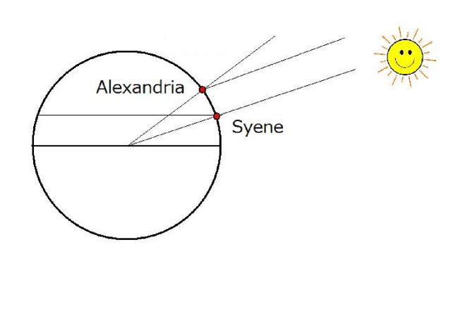
Prominent among them is Eratosthenes of Cyrene (ca. 276 BCE–ca. 195 BCE), the third chief librarian appointed by Ptolemy II and famous for an algorithm for finding all prime numbers.242424Archimedes’ Method mentioned in fn. 12 takes the form of a letter to Eratosthenes. Pushing further the view about the spherical earth, he adroitly calculated the meridian of the earth. The outcome was 46,620 km, about 16% greater than the actual value. His work On the measurement of the earth was lost, but the book On the circular motions of the celestial bodies by Cleomedes (died ca. 489 CE) explains Eratosthenes’ deduction relying on a property of parallels and the observation that at noon on the summer solstice, the sun casts no shadow in Syene (now Aswan), while it casts a shadow on one fiftieth of a circle ( degree) in Alexandria on the same degree of longitude as Syene (Fig. 2). His resulting value is deduced from the distance between the two cities (5040 stades925 km), which he inferred from the number of days that caravans require for travelling between them.
The Ptolemaic dynasty lasted until the Roman conquest of Egypt in 30 BCE, but even afterwards Alexandria maintained its position as the center of scientific activity (see Sect. 11).
Finishing the excursion into ancient times, we shall turn back to the later stage of the Renaissance, the age that science was progressively separated from theology, and scientists came to direct their attention to scientific evidence rather than to theological accounts (thus science was becoming an occasional annoyance to the religious authorities). Representative in this period (religiously tumultuous times) are the Catholic Galileo and the Protestant Johannes Kepler (1571–1630); both gave a final death blow to Aristotelian/Ptolemaic theory.
Kepler discovered the three laws of planetary motion, based on the data of Mars’ motion recorded by Tycho Brahe (1546–1601).252525Tycho Brahe, the last of the major naked-eye astronomers, rejected the heliocentricism. His model of the universe is a combination of the Ptolemaic and the Copernican systems, in which the planets revolved around the Sun, which in turn moved around the stationary Earth. His first and second laws were elaborated in the Astronomia nova (1609). The first law asserts that the orbit of a planet is elliptical in shape with the center of the sun being located at one focus. The second law says that a line segment joining the sun and a planet sweeps out equal areas in equal intervals of time. The third law stated in the Epitome Astronomiae Copernicanae (1617–1621) and the Harmonices Mundi (1619) maintains that the square of the orbital period of a planet is proportional to the cube of the semi-major axis of its orbit.
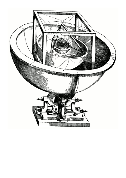
Before this epoch-making discovery, however, he attempted to explain the distances in the Solar system by means of “regular convex polyhedra” inscribing and circumscribed by spheres, where the six spheres separating those solids correspond to Saturn, Jupiter, Mars, Earth, Venus, and Mercury (Mysterium Cosmographicum, 1596; Fig. 3). He also rejected the infiniteness of the universe, on the basis of an astronomical speculation on the one hand, and on the traditional scholastic doctrine on the other (for this reason, Kepler is portrayed as the last astronomer of the Renaissance, and not the first of the new age).
Galileo was not affected by Aristotelian prejudice that an experiment was an interference with the natural course of Nature. Without performing any experiment at all, medieval successors of Aristotle insisted, for instance, that a projectile is pushed along by the force they called “impetus,” and if the impetus is expended, the object should fall straight to the ground. At the apogee of his scientific career, Galileo had conducted experiments on projectile motion, and observed that their trajectories are always parabolic (1604–1608). He further investigated the relation between the distance an object (say, a ball) falls and the time that passes during the fall, and found the formula (in modern terms), where , the gravitational acceleration (Discorsi). The crux of this formula is that the drop distance does not depend on the mass of a falling object, contrary to Aristotle’s prediction (Physics, IV, 8, 215a25).262626The mean speed theorem due to the Oxford Calculators (nothing but the formula for the area of a trapezoid from today’s view) is a precursor of “the law of falling bodies.”
Galileo turned his eyes on the universe. With his handmade telescope, he made various astronomical observations and confirmed that four moons orbited Jupiter. This prompted him to defend the heliocentricism, for provided that Aristotle were right about all things orbiting earth, these moons could not exist (Sidereus Nuncius, 1610). As an inevitable consequence, his Copernican view led to the condemnation at the Inquisition (1616, 1633). After being forced to racant, he was thrown into a more thorny position than Kepler, and had to avoid dangerous issues that may provoke the Church. Regarding the size of the universe, he denied the existence of the celestial sphere as the limit, while he was reluctant to say definitely that the universe is infinite, because of censorship by the Church. In a letter to F. Liceti on February 10, 1640, Galileo says, “the question about the size of the universe is beyond human knowledge; it can be only answered by the Bible and a divine revelation.”
Next to Kepler and Galileo are Descartes and Pascal, the intellectual heroes of 17th-century France, who laid the starting point of the Enlightenment with their inquiries into truth and the limits of reason.
René Descartes (1596–1650), whose natural philosophy agrees in broad lines with Galileo’s one, defended the heliocentrism, by saying that it is much simpler and distinct, but hesitated to make his opinion public upon the news of the Inquisition’s conviction of Galileo (1633). As regards the size of the universe, he maintained at first that the universe is finite; but later became ambivalent. In a letter in 1649 to the rationalist theologian H. More of Cambridge, he conceded, after a long dispute, that the universe must have infinite expanse because one cannot think of the limit; for if the limit exists, one cannot help but think of the outside of space which must be the same as our space.
While, for Descartes, the self is prior and independent of any knowledge of the world, Blaise Pascal (1623–1662) pronounced that the order is reversed; that is, knowledge of the world is a prerequisite to knowledge of the self. In the Pensées (1670), in comparison with the disproportion between our justice and God’s, he writes, “Unity added to infinity does not increase it at all [….]: the finite is annihilated in the presence of the infinite and becomes pure nothingness” (fragment 418). Further, he says, “Nature is an infinite sphere of which the center is everywhere and the circumference nowhere” (fragment 199).272727This sentence, reminiscent of Cusanus’ view, may be from the Liber XXIV philosophorum (Book of the 24 Philosophers), an influential philosophical and theological medieval text, usually attributed to Hermes Trismegistus, the purported author of the Corpus Hermeticum.
As described hitherto, the posture to pay attention to the universe is a steady tradition of European culture. In its background, philosophy was nurtured in the bosom of cosmogony, and could not be separated from religion because of the intimacy between them. Especially after the rise of Christianity, Western scholars had to be confronted, at the risk of their life in the worst case, with God as a creator. Even after the tension between science and religion was eased, scientists could not be entirely free from God, whatever His image is. Such milieu led quite naturally to probing questions about our universe in return.
In summary, “whether the universe is finite or infinite,” whatever it means, is an esoteric issue in religion, metaphysics, and astronomy in Europe that had intrigued and baffled mankind since dim antiquity. What matters most of all is whether the outside is necessary when we talk about finiteness of the universe.
4 From Descartes to Newton and Leibniz
Intuition for space surrounding us was the driving force for people to puff up their image of the universe. Needless to say, from the ancient times to the Middle Ages and even the early modern times, the mental image that nearly all people had is, if not being particularly conscious about it, the one described by Euclidean space, the model of our space named after the Alexandrian Euclid (Ε’υϰλείδης; ca. 300 BCE; see Sect. 9 for the details). Even the advocates of the spherical model of the universe imagined Euclidean space as the entity embracing all. Synthetic geometry executed on this model is what we call Euclidean geometry. It started with a collection of geometrical results acquired in Egypt and Mesopotamia by empirical investigations or experience of land surveys and constructions of magnificent and imposing structures, and had been systemized, as the search of universals, through the efforts of Greek geometers.
Putting it briefly, Euclidean space is homogeneous in the sense that there is no special place, and it is isotropic; i.e., there is no special direction.282828Euclidean space holds one more significant aspect expressed by a property of parallels, but its true meaning had not been comprehended for quite a while; see Sect. 10. These features are not expressly indicated in Greek geometry, but are guaranteed by a property of congruence;292929 Prop. 4 in the Elements, Book I, is the first of the congruence propositions. namely any geometric figure can be rotated and moved to an arbitrary place while keeping its shape and size. What should be pinpointed here is that it was not until the 19th century that people explicitly conceptualized Euclidean space (or space as a mathematical object which fits in with our spatial intuition). Until then, geometry meant only Euclidean geometry, and the space where geometry is performed was considered as an a priori entity, or what amounts to the same thing, our space—a place of storage in which objects are recognized, and a place of manufacture in which objects are constructed—was not an entity for which we investigate whether our understanding of it is right or wrong, thereby all the propositions of geometry being considered “absolute truth.”
As stated above, Euclidean geometry had been a lofty edifice for nearly 2000 years that nobody could break down. Only the appearance changed when Descartes invented the so-called algebraic method. This epoch-making method is elucidated in his La Géométrie [5], one of the three essays attached to the philosophical and autobiographical treatise Discours de la méthode pour bien conduire sa raison, et chercher la vérité dans les sciences (1637).303030La Géométrie consists of Book I (Des problèmes qu’on peut construire sans y employer que des cercles et des lignes droites), Book II (De la nature des lignes courbes), and Book III (De la construction des problèmes solides ou plus que solides). The other two essays are La Dioptrique and Les Météores.
Descartes’ prime concern was, though he was trained in religion with the still-authoritarian nature, to find principles that one can know as true without any scruples. In the self-imposed search for certainty, he linked philosophy with science, and had the confidence that certainty could be found in the mathematical proofs having the apodictic character. Upon his emphasis on lucid methodology and dissatisfaction with the ancient arcane method, as already glimpsed in his Regulae ad Directionem Ingenii (1628), he attempted to create “universal mathematics” by bridging the gap between arithmetic and geometry that used to be thought of as different terrains. Indeed, the Greeks definitely distinguished geometric quantities from numerical values, and even thought that length, area, and volume belong to different categories, thus lumping them together makes no sense. Under such shackles (and being devoid of symbolic algebra), the “equality,” “addition/subtraction,” and the “large/small relation” for two figures in the same category were defined by means of geometric operations.313131The Greeks had difficulty to handle irrationals in their arithmetic and were forced to replace algebraic manipulations by geometric ones ([22]). Actually, geometry had been thought of as far more general than arithmetic as seen in Aristotle’s words, “We cannot prove geometric truths by arithmetic” (Posterior Analytics, I, 7; see also Plato’s Philebus, 56d). The word “algebra,” stemmed from the Arabic title al-Kit al-mukhtasar fi hisb al-jabr walmuqbala (The Compendious Book on Calculation by Completion and Balancing) of the book written approximately 830 CE by al-Khwrizmī (ca. 780–ca. 850) (Remark 2.1 (2)), was first imported into Europe in the early Middle Ages as a medical term, meaning “the joining together of what is broken.” In addition, algorithm, meaning a process to be followed in calculations, is a transliteration of his surname al-Khwrizmī. Specifically, they considered that two polygons (resp. polyhedra) are “equal” if they are scissors-congruent; i.e., if the first can be cut into finitely many polygonal (resp. polyhedral) pieces that can be reassembled to yield the second.
Remark 4.1
Any two polygons with the same numerical area are scissors-congruent as shown independently by W. Wallace in 1807, Farkas Bolyai in 1832, and P. Gerwien in 1833. Gauss questioned whether this is the case for polyhedra in two letters to his former student C. L. Gerling dated 8 and 17 April, 1844 (Werke, VIII, 241–42). In 1900, Hilbert put Gauss’s question as the third problem in his list of the 23 open problems at the second ICM. M. W. Dehn, a student of Hilbert, found two tetrahedra with the same volume, but non-scissors-congruent (1901); see [37].
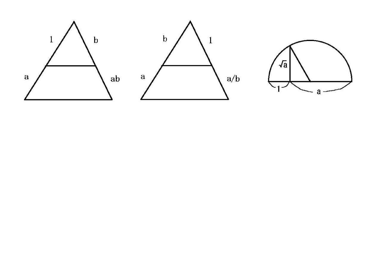
In his essay La Géométrie, Descartes made public that all kinds of geometric magnitude can be unified by representing them as line segments, and introduced the fundamental rules of calculation in this framework.323232A letter dated March 26, 1619 to I. Beeckman indicates that Descartes already held a rough scheme at the age of 22. Pierre de Fermat (1601–1665) argued a similar idea in his Ad locos plano et solidos isagoge (1636), though not published in his life time. His idea is to fix a unit length, with which he defines addition, subtraction, multiplication, division, and the extraction of roots for segments, appealing to the proportional relations of similar triangles and the Pythagorean Theorem, as indicated in Fig. 4. Then he adopts a single axis to represent these operations; thereby replacing the Greek geometric algebra by “numerical” algebra. On this basic format, he handles various problems for a class of algebraic curves. Priding himself on his invention, he says, in a fond familiar letter dated November 1643 to Elisabeth (Princess Palatine of Bohemia), that extra effort to make up the constructions and proofs by means of Euclid’s theorems is no more than a poor excuse for self-congratulation of petty geometers because such effort does not require any scientific mind.
Afterwards, Franciscus van Schooten (1615–1660), who met Descartes in Leiden (1632) and read the still-unpublished La Géométrie, translated the French text into Latin, and endeavored to disseminate the algebraic method to the scientific community (1649). In the second edition (1659–61), he added annotations and transformed Descartes’ approach into a systematic theory, which made it far more accessible to a large number of audience.
Descartes’ method, along with algebraic notations dating back to François Viète (1540–1603) who made a momentous step towards modern algebra,333333Viète, In artem analyticem isagoge (1591). was inherited as analytic geometry afterwards. With this progression, geometric figures were to be transplanted to algebraic objects in the coordinate plane or the coordinate space .343434It was Leibniz who first introduced the “coordinate system” in its present sense (De linea ex lineis numero infinitis ordinatim ductis inter se concurrentibus formata, easque omnes tangente, ac de novo in ea re Analysis infinitorum usu, Acta Eruditorum, 11 (1692), 168–171). Incidentally, Oresme used constructions similar to rectangular coordinates in the Questiones super geometriam Euclidis and Tractatus de configurationibus qualitatum et motuum (ca. 1370), but there is no evidence of linking algebra and geometry. What is more, this new discipline was integrally connected with the calculus initiated by Issac Newton (1642–1726) and Gottfried Wilhelm von Leibniz (1646–1716), independently and almost simultaneously, which is to be a vital necessity when we talk about the shape of our universe.
Newton learnt much from the Exercitationes mathematicae libri quinque (1657) by van Schooten and Clavis Mathematicae (1631) by William Oughtred (1574–1660) when he was a student of Trinity College, Cambridge. “Fluxion” is Newton’s underlying term in his differential calculus, meaning the instantaneous rate of change of a fluent, a varying (flowing) quantity. His idea, to which Newton was led by personal communication with Issac Barrow (1630–1677) and also by Wallis’ book Arithmetica infinitorum (1656),353535John Wallis (1616–1703) propagated Descartes’ idea in Great Britain through his work. is stated in two manuscripts; one is of October 1666 written when he was evacuated in a neighborhood of his family home at Woolsthorpe during the Great Plague, and another is the Tractatus De Methodis Serierum et Fluxionum (1671). In his calculus, Newton made use of power series in a systematic way.
Meanwhile, Leibniz almost completed calculus while staying in Paris (1673–1676) as a diplomat of the Electorate of Mainz in order to get Germany back on its feet from the exhaustion caused by the Thirty Years’ War. Although the aspired end of diplomacy was not attained, he had an opportunity to meet Christiaan Huygens (1629–1695), a leading scientist of his time, who happened to be invited by Louis XIV as a founding member of the Académie des Sciences. Very helpful for him was the suggestion by Huygens to read Pascal’s Lettre de Monsieur Dettonville (1658). Further, his perusal of Descartes’ work was an assistance in strengthening the basis of his thought. Around the time when Leibniz returned to Germany, he improved the presentation of calculus, and brought it out as two papers; Nova methodus pro maximis et minimis, and De geometria recondita et analysi indivisibilium atque infinitorum.363636His papers were published in Acta Eruditorum, 3 (1684), 467–473 and 5 (1686), 292–300. In the second paper, he states, “With this idea, geometry will make a far more greater strides than Viète’s and Descartes’.”
Their calculus, though still something of mystery (Remark 15.1 (2)), provided a powerful tool which enabled to handle more complicated geometric figures than the ones that Greek geometers treated in an ad hoc manner.373737In the Elements, Book III, Def. 2, Euclid says, “a straight line is said to touch a circle which, meeting the circle and being produced, does not cut the circle.” Curiously, in the Metaphysics, III, 998a, Aristotle reports that Protagoras (ca. 490 BCE–ca. 420 BCE) argued against geometry that a straight line cannot be perceived to touch a circle at only one point. Indeed, differential calculus provides a unified recipe to find tangents of a general curve (say, transcendental curves Descartes did not deal with), and integral calculus (called the “inverse tangent problem” by Leibniz) allows more latitude in calculating the area of a general figure without any ingenious trick. Paramountly important is the discovery that tangent (a local concept) and area (a global concept) are linked through the fundamental theorem of calculus (FTC).383838I. Barrow, who strongly opposed to Descartes’ method in contrast with Wallis, knew the FTC in a geometric form (Prop. 11, Lecture 10 of his Lectiones Geometricae delivered in 1664–1666). A transparent proof was given by Leibniz in his De geometria, 1686.
There are other lines of evolution of Descartes’ method and its offspring. Analytic geometry paved the way for higher-dimensional geometry (Sect. 14), which was to be incorporated into Riemann’s theory of curved spaces (Sect. 15). Algebraic geometry is regarded as the ultimate incarnation of Cartesian geometry, which came of age from the late 19th century to the early 20th century. Descartes’ method also prompted to set up mathematical theories in a strictly logical manner, not relying on geometry, but relying on arithmetic wherein concepts involved are entirely framed in the language of real numbers or systems of such (Sect. 16). This signifies in some sense that mathematicians eventually become aware of mathematical reality—a sort of Plato’s world of Forms (είδος or its cognates)—distinguished from physical reality or the empirical world.
Remark 4.2
(1) Symbols and symbolization has played a significant role in the history of mathematics. Prior to Viète, the symbols were used by H. Grammateus in Ayn new Kunstlich Buech (1518). Actually, these symbols already appeared in 1489 to indicate surplus and deficit for the mercantile purpose. In 1525, the symbol was invented by C. Rudolff, a student of Grammateus. Subsequently, R. Recorde adopted the equal sign in 1557. After Viète, Oughtred innovated the symbol for multiplication in his Clavis Mathematicae (1631). In the same year, the book Artis analyticae praxis ad aequationes algebraicas resolvendas by Thomas Harriot (ca. 1560 –1621), which left a great mark on the history of symbolic algebras, was brought out posthumously, wherein the symbols “” representing the magnitude relation appear. For all of this, the usage of symbols in Descartes’ time was almost in agreement with that of today.
(2) When integral calculus was still in its nascent stage, Kepler computed the volumes of solids of revolution.393939Nova stereometria doliorum vinariorum (1615). After a while, Bonaventura Cavalieri (1598–1647), a disciple of Galileo, proposed a naive but a systematic method, known as Cavalieri’s principle, to find areas and volumes of general figures, which is thought of as intermediating between the Greek quadrature and integral calculus.404040Geometria indivisibilibus continuorum nova quadam ratione promota (1635, 1653). The linchpin of his innovation is the notion of indivisibles; he regards, for instance, a plane region as being composed of an infinite number of parallel lines, each considered to be an infinitesimally thin rectangle.
(3) Although calculus initiated by Newton and Leibniz was the same in essence, their styles differed in a crucial way. The difference was reflected in the notation they used. For instance, Leibniz invented the symbol , while Newton employed the dot notation . This difference arose, as often said, that the British mathematics under a baneful influence of Newton’s authority had fallen seriously behind the Continental counterpart. They were jolted by the Mécanique Céleste by Pierre-Simon Laplace (1749–1827) which was affiliated with the “Leibnizian school.” John Playfair (1748–1819) says, “We will venture to say that the number of those in this island who can read the Mécanique Céleste with any tolerable facility is small indeed” (1808).
(4) Until the 19th century through a pre-classical theory implicit in the work of Newton, Leibniz and their successors, real numbers had been grasped as points on a straight line—the vision that dates back to Descartes and is credited to J. Wallis—or “something” (without telling what they are) approximated by rational numbers.414141Simon Stevin (1548-1620) renovated the notation for decimal fractions to make all computations easier, which contributed to the apprehension of the nature of real numbers. In the 35-page booklet De Thiende (1585), he expressed by 27847 for instance.
Thus calculus had been built on a fragile base. In a letter to his benefactor dated March 29, 1826, Niels Henrik Abel (1802–1829) writes, “the tremendous obscurity one undoubtedly finds in analysis today. It lacks all plan and system [] The worst of it is, it has never been treated with rigor. There are very few theorems in advanced analysis that have been demonstrated with complete rigor” (Remark 19.1).
An entrenched foundation to calculus was furnished by Richard Dedekind (1831–1916). He constructed the real number system by appealing to what we now call the method of Dedekind cuts, partitions of the rational numbers into two sets such that all numbers in one set are smaller than all numbers in the other (1872).424242 In the same year, Cantor arrived at another definition of the real numbers (fn. 147). To say the least, this understanding heralds the emancipation of analysis from geometry.
Long ago, Eudoxus developed an idea similar to Dedekind’s in essence. Before that, Greek geometers had tacitly assumed that two magnitudes , are always commensurable (ς´υμμετρος); i.e., there exist two natural numbers such that . Thus, with the discovery of incommensurable magnitudes which results from the Pythagorean Theorem, the issue arose as to how to define equality of two ratios. The impeccable definition attributed to Eudoxus is : “Magnitudes are said to be in the same ratio, the first to the second and the third to the fourth, when, if any equimultiples whatever are taken of the first and third, and any equimultiples whatever of the second and fourth, the former equimultiples alike exceed, are alike equal to, or alike fall short of, the latter equimultiples respectively taken in corresponding order” ([7], Book V, p.114). In modern terminology, this is expressed as “Given four magnitudes , the two ratios and are said to be the same if for all natural numbers , it be the case that according as , so also is .”
Related to the theory of proportions is the anthyphairesis (ἀνϑυφαίρεςις), a method to find the ratio of two magnitudes. A special case is Euclid’s algorithm used to compute the greatest common divisors of two numbers (Elements, Book VII, Prop. 2; see [20]). Specifically, for two magnitudes , it proceeds as (Book X, Prop. 2). Here, and are commensurable if and only if this process terminates after a finite number of steps (i.e., for some ). This idea was handed down to us as the technique to obtain continued-fraction expansions afterward. Namely, for positive real numbers , eliminating in the above, we have
.
5 A new approach in classical geometry
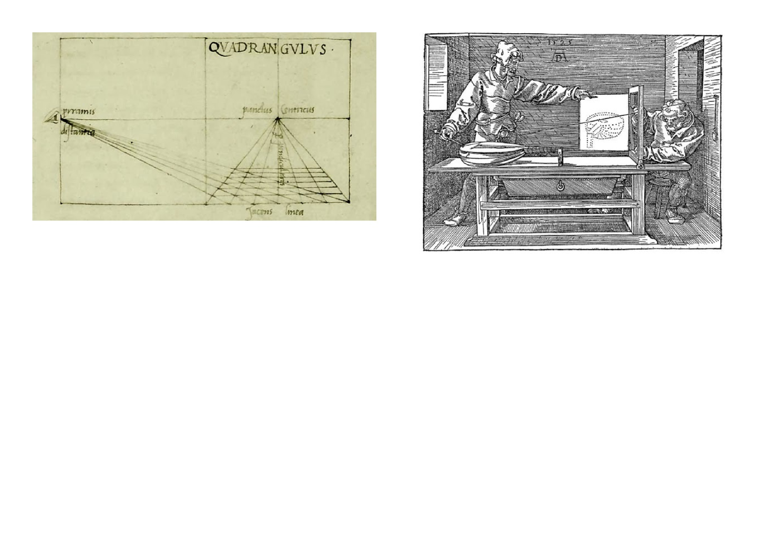
Leaving Euclidean geometry aside for a moment, we shall touch on projective geometry, the embryonic subject that came up during the Renaissance period and had matured in the 19th century. This new approach is exclusively concerned with quantity-independent properties such as “three points are on a line” (collinearity) and “three lines intersect at a point” (concurrency) that are invariant under projective transformations (the left of Fig. 5).434343 Imitating this wording, one may say that Euclidean geometry is a geometry that treats invariant properties under congruence transformations. Such a perspective is ascribed to Christian Felix Klein (1849–1925), who promulgated his scheme in the booklet Vergleichende Betrachtungen über neuere geometrische Forschungen (“Erlangen Program” in short) in 1872.
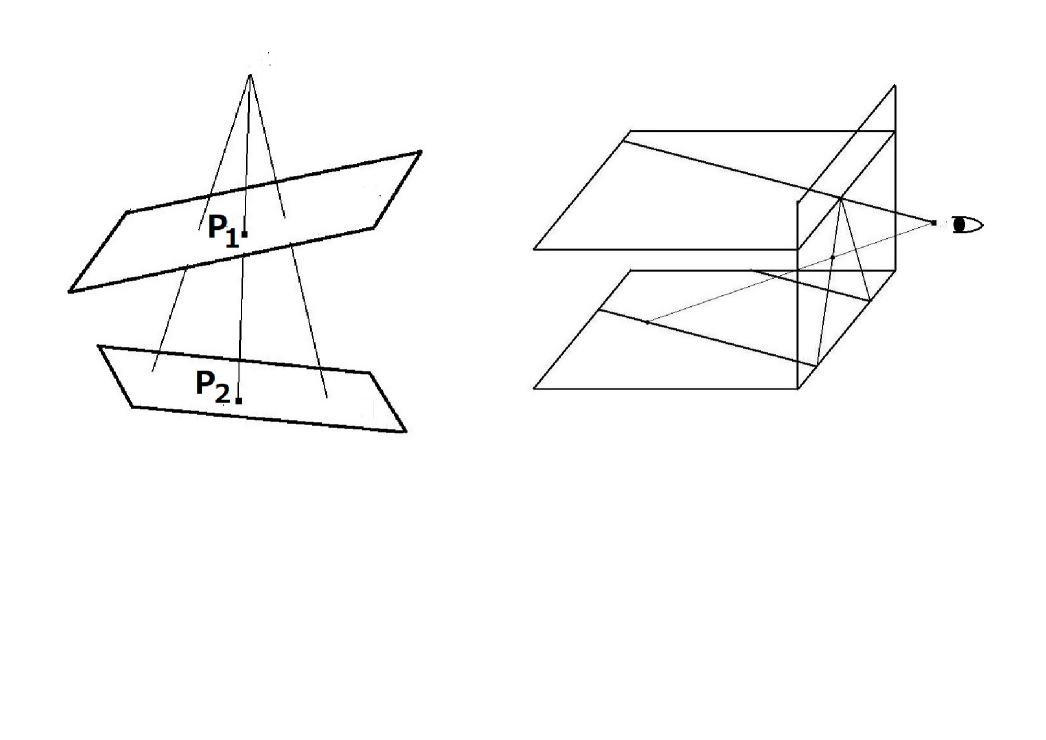
Projective geometry has a historical link to (linear) perspective, an innovative skill in drawing contrived by Filippo Brunelleschi(1377–1446), which allowed Renaissance artists to portray a thing in space and landscapes as someone actually might see them.444444One of the earliest who have used perspective is Masaccio. He limned the San Giovenale Triptych (1422) based on the principles he learned from Brunelleschi, which emblematizes the transition from medieval mysticism to the Renaissance spirit. The theoretical aspect of perspective was investigated by Leon Battista Alberti (1404–1472) and Piero della Francesca (1416–1492). In the preface of his book Della Pittura (1435) dedicated to Brunelleschi, Alberti emphatically writes, “I used to marvel and at the same time to grieve that so many excellent and superior arts and sciences from our most vigorous antique past could now seem lacking and almost wholly lost. Since this work [due to Brunelleschi] seems impossible of execution in our time, if I judge rightly, it was probably unknown and unthought of among the Ancients” (translated by J. R. Spencer). Piero’s book De Prospectiva Pingendi (1475) exemplifies the effective symbiosis of geometry and art; he actually had profound knowledge of Greek geometry and made a transcription of a Latin translation of Archimedes’ work.
The “Renaissance Man” Leonardo da Vinci (1452–1519)—stimulated by Alberti’s book—fully deserves his reputation as a true master of perspective. His technique is particularly seen in his study for A Magis adoratur (ca. 1481). He says, “Perspective is nothing else than seeing a place or objects behind a plane of glass, quite transparent, on the surface of which the objects behind the glass are to be drawn” ([30]). Albrecht Dürer (1471–1528), a weighty figure of the Northern Renaissance who shared da Vinci’s pursuit of art, discussed in his work Underweysung der Messung (1525) an assortment of mechanisms for drawing in perspective from models (the right of Fig. 6). This work, in which he touched on “Doubling the cube,” is the first on advanced mathematics in German.
Subsequently, Federico Commandino (1506–1575) published the work entitled Commentarius in planisphaerium Ptolemaei (1558). This, a commentary on Ptolemy’s work Planisphaerium, includes an account of the stereographic projection of the celestial sphere, and is a work on perspective from a mathematical viewpoint (concurrently, he translated several work of ancient scholars).
Remark 5.1
Da Vinci drew the illustrations of the regular polyhedra in the book De divina proportione (1509) by Fra Luca Bartolomeo de Pacioli (ca. 1447–1517), a pupil of Piero. The theme of the book is mathematical and artistic proportions, especially the golden ratio—the positive solution of the equation —and its application in architecture. The golden ratio appears in the Elements, Book II, Prop. 11; Book IV, Prop. 10–11; Book XIII, Prop. 1-–6, 8-–11, 16-–18,454545In Book VI, Def. 3, Euclid says, “A straight line is said to have been cut in extreme and mean ratio (ἄϰρος ϰαὶ μέςος λ´ογος) when, as the whole line is to the greater segment, so is the greater to the less.” In today’s terms, “the segment is cut at in extreme and mean ratio when .” Note that equals the golden ratio. Kepler, who proved that is the limit of the ratio of consecutive numbers in the Fibonacci sequence, described it as “a fundamental tool for God in creating the universe” (Mysterium Cosmographicum). and is commonly represented by the Greek letter after the sculptor Pheidias (Φειδίας, ca. 480 BCE–ca. 430 BCE) who is said to have employed it in his work.
The origin of projective geometry can be traced back to the work of Apollonius of Perga on conic sections and Pappus of Alexandria (ca. 290 CE–ca. 350 CE).464646The first who studied conic sections is Menaechmus (ca.380 BCE–ca.320 BCE), who used them to solve “doubling the cube.” The names ellipse (ἔλλειψις), parabola (παραβολη) and hyperbola (´υπερβολη) for conic curves were introduced by Apollonius. In his Collection, Book VII, where Pappus enunciated his hexagon theorem, he made use of a concept equivalent to what we call now the cross-ratio, which was to enrich projective geometry from the quantitative side since it is invariant under projective transformations. Here the cross-ratio of collinear points , , and is defined as , where each of the distances is signed according to a consistent orientation of the line.474747The cross-ratio of real numbers is defined by . The projective invariance of cross-ratios amounts to the identity , where .
Projective geometry as a solid discipline was essentially initiated by Girard Desargues (1591–1661), a coeval of Descartes. In 1639, motivated by a practical purpose pertinent to perspective, he published the Brouillon project d’une atteinte aux événemens des rencontres du Cone avec un Plan.484848The celebrated Desargues’ theorem showed up in an appendix of the book Exemple de l’une des manières universelles du S.G.D.L. touchant la pratique de la perspective published in 1648 by his friend A. Bosse. Pascal took a strong interest in Desargues’ work, and studied conic sections in depth at the age of 16. Philippe de La Hire (1640–1718) was affected by Desargues’ work, too. He is most noted for the work Sectiones Conicae in novem libros distributatae (1685). However, partly because Descartes’ method spread among the mathematical community in those days and because of his peculiar style of writing, his work remained unrecognized until his work was republished in 1864 by Noël-Germinal Poudra. Without being aware of Desargues’ work, Jean-Victor Poncelet (1788–1867) laid a firm foundation for projective geometry in his masterpiece Traité des propriétés projectives des figures (1822).
In any case, projective geometry falls within classical geometry at this moment; but it has an interesting hallmark in view of infiniteness. Guidobaldi del Monte (1505–1607) in the Perspectivae Libri VI (1600) and Kepler in his Astronomiae pars optica (1604) proposed the idea of points at infinity. Subsequently, having in mind the “horizon” in perspective drawing (Fig. 5), Desargues appends points at infinity to the plane as idealized limiting points at the “end,” and argues that two parallel lines intersect at a point at infinity. Later, the “plane plus points at infinity” came to be termed the projective plane (Sect. 16).
6 Euclid’s legacy in physics and philosophy
Not surprisingly, Euclidean geometry predominated in physics for a long time. Salient is Newton who adopted Euclidean geometry as the base of his grand work Philosophiae Naturalis Principia Mathematica (1687, 1713, 1726; briefly called the Principia), in which he formulated the law of inertia,494949The law of inertia was essentially discovered by Galileo during the first decade of the 17th century though he did not understand the law in the general way (the term “inertia” was first introduced by Kepler in his Epitome Astronomiae Copernicanae). The general formulation of the law was devised by Galileo’s pupils and Descartes (the Principles of Philosophy, 1644). the law of motion, the law of action-reaction and the law of universal gravitation.
It was in 1666, exactly the same year when he worked out calculus, that Newton found a clue leading to the law of universal gravitation. Hagiography has it that he was inspired, in a stroke of genius, to formulate the law while watching the fall of an apple from a tree. Leaving aside whether this is a fact or not, all we can definitely say is, he concluded that the force acting on objects on the ground (say, apples) acts on the moon as well; he thus found the extraordinarily significant connection between the terrestrial and celestial which had been thought of as being independent of each other.
To go further with his subsequent observation, let be the center of the earth, and let be the position of the moon. We denote by and the speed and acceleration of , respectively. The acceleration is directed towards , and , where is the distance between and . If the orbital period of the moon is , then , so that . Next, applying Kepler’s third law to a circular motion, we have . Hence and , which is the force acting on in view of the law of motion, and the law of universal gravitation follows. Conversely, based on his laws, Newton derived Kepler’s laws through far-reaching deductions.505050Newton tried to reconfirm his theory of gravitation by explaining the motion of the moon observed by J. Flamsteed, but the 3-body problem for the Moon, Earth and Sun turned out be too much complicated to accomplish his goal (he planned to carry a desired result as a centerpiece in the new edition of the Principia).
Remark 6.1
We let be the position of a point mass (particle) in motion at time . The law of motion is expressed as , where is the inertial mass of the particle, and stands for a force. The law of universal gravitation says that a point mass fixed at the origin attracts the point mass at by the force ,515151Throughout, and stand for norm and inner product, respectively. where is the gravitational constant, and is the gravitational mass at the origin. What should be stressed is, as stated in the opening paragraph of the Principia, that the inertial mass coincides with the gravitational mass under a suitable system of units (this is by no means self-evident), so that the Newtonian equation is expressed as , namely, the acceleration does not depend on the mass as Galileo observed for a falling object. Kepler’s laws of planetary motion are deduced from this equation.
The Newton’s cardinal importance in the history of cosmology lies in his understanding of physical space. According to him, Euclidean space is an “absolute space,” with which one can say that an object must be either in a state of absolute rest or moving at some absolute speed. To justify this, he assumed that the fixed stars can be a basis of “inertial frame.” His bucket experiment,525252When a bucket of water hung by a long cord is twisted and released, the surface of water, initially being flat, is eventually distorted into a paraboloid-like shape by the effect of centrifugal force. This shape shows that the water is rotating as well, despite the fact that the water is at rest relative to the bucket. From this, Newton concluded that the force applied to water does not depend on the relative motion between the bucket and the water, but it results from the absolute rotation of water in the stationary absolute space (fn. 187). elucidated in the Scholium to Book 1 of the Principia, is an attempt to support the existence of absolute motion.
Setting aside the theoretical matters, what is peculiar about the Principia is that Newton adhered to the Euclidean style, and used laboriously the traditional theory of proportions in Book V of the Elements and the results in Apollonius’ Conics even though he was well acquainted with Descartes’ work, which was, as a matter of course, more appropriate for the presentation. He testified, writing about himself in the third person, “By the help of the Analysis, Mr. Newton found out most of Propositions of his Principia Philosophiae: but because the Ancients for making things certain admitted nothing into Geometry before it was demonstrated synthetically, he demonstrated the Propositions synthetically, that the System of Heavens might be founded upon good Geometry. And this makes it now difficult for unskillful Men to see the Analysis by which those Propositions were found out” (Phil. Trans. R. Soc., 29 (1715), 173–224).
Apart from the style of the Principia, this epoch-making work (and its offspring) was “the theory of everything” in the centuries to follow as far as the classical description of the world is concerned. Indeed, Newton’s laws seemed to tap all the secrets of nature, and hence to be the last word in physics. It was in the 19th century that physical phenomena inexplicable by the Newtonian mechanics were discovered one after another. A notable example is electromagnetic phenomena which are in discord with his mechanics in the fundamental level; see Remark 17.2 (4). Moreover various physicochemical phenomena called for entirely new explanations as well, and eventually led to quantum physics.
Newton was a pious Unitarian. His theological thought had him say, “Space is God’s boundless uniform sensorium.”535353The medieval tradition had so much effect on Newton that he was deeply involved in alchemy and regarded the universe as a cryptogram set by God. As J. M. Keynes says, he was not the first of the age of reason, but the last of the magicians (Newton the Man, 1947). This gratuitous comment to his own comprehensive theory provoked a criticism from Leibniz, who said that God does not need a sense organ to perceive objects. Moreover, on the basis of “the principle of sufficient reason” and “the principle of the identity of indiscernibles,” Leibniz claimed that space is merely relations between objects, thereby no absolute location in space, and that time is order of succession. His thought was unfolded in a series of long letters between 1715 and 1716 to a friend of Newton, S. Clarke.545454Clarke (1717), A Collection of Papers, which passed between the late Learned Mr. Leibniz, and Dr. Clarke, In the Years 1715 and 1716. Having said that, however, the existence of God is an issue which Leibniz could not sidestep. To be specific, his principle of sufficient reason made him assert that nothing happens without a reason, and that all reasons are ex hypothesi God’s reasons. One may ask, for instance, “Why would God have created the universe here, rather than somewhere else?” That is, when God created the universe, He had an infinite number of choices. According to Leibniz, He would choose the best one among different possible worlds. As will be explained later (Sect. 12), his insistence, though having a strong theological inclination, is relevant to a fundamental physical principle.
At all events, the period that begins with Newton and Leibniz corresponds to the commencement of the close relationship between mathematics and physics. From then on, both disciplines have securely influenced each other.
Immanuel Kant (1724–1804), who stimulated the birth of German idealism, was influenced by the rationalist philosophy represented by Descartes and Leibniz on the one hand, and troubled by Hume’s thoroughgoing skepticism on the other.555555The empiricist David Hume is a successor of F. Bacon, T. Hobbes, J. Locke, and G. Berkeley. He says that an orderly universe does not necessarily prove the existence of God (An Enquiry Concerning Human Understanding, 1748). Hobbes, an Aristotle’s critic, described the world as mere “matter in motion,” maybe the most colorless depiction of the universe since the ancient atomists, but he did not abandon God in his cosmology (Leviathan, 1651). He felt the need to rebuild metaphysics to argue against Hume’s view. Being also dissatisfied with the state of affairs surrounding metaphysics, in contrast to the scientific model cultivated in his days, Kant strove to lay his philosophical foundation of reason and judgement on secure grounds.
He was an enthusiast of Newtonian physics framed on Euclidean geometry, and asked himself, “Are space and time real existences? Are they only determinations or relations of things as Leibniz insists?” His inquiry brought him to the conclusion that Euclidean geometry is the inevitable necessity of thought and inherent in nature because our space (as an “absolute” entity) is a “sacrosanct” framework for all and any experience. He also held that space (as a “relative” entity) is the “subjective constitution of the mind” (see Sect. 22), He stressed further that mathematical propositions are formal descriptions of the a priori structures of space and time.565656Affected by the science in his time, Kant developed further the nebular hypothesis proposed by E. Swedenborg in 1734 (this hypothesis that the solar system condensed from a cloud of rotating gas was discussed later by Laplace in 1796).
In the work Allgemeine Naturgeschichte und Theorie des Himmels (1755), Kant discussed infiniteness of the universe. He believed that the universe is infinite, because God is the “infinite being,” and creates the universe in proportion to his power (recall Bruno’s view). In turn, he argues that it is not philosophically possible to decide whether the universe is infinite or finite; that is, we are incapable of perceiving so large distance, because the mind is finite.575757Hegel dismissed the claim that the universe extends infinitely.
As Kant emphasized in the Kritik der reinen Vernunft (1781), abstract speculation must be pursued without losing touch with reality grasped by intuition; otherwise the outcome could be empty. This is not least the case for scientific knowledge. Yet intuition about our space turned out to be a clinging constraint on us; it was not easy to free ourselves from it.
7 Gauss –Intrinsic description of the universe
In Christianity, God is portrayed to be omnipresent, yet His whereabouts is unknown. Nonetheless, the laity usually personify God (if not a person literally), and believe that He “dwells” outside the universe (or empyrean). Imagining such a deity is not altogether extravagant from the view that we will take up in investigating a model of the universe though we do not posit the existence of God. What is available in place of God is, of course, mathematics.585858Robert Grosseteste (ca. 1175–1253) in medieval Oxford says, “mathematics is the most supreme of all sciences since every natural science ultimately depends on it” (De Luce, 1225). He maintained, by the way, that stars and planets in a set of nested spheres around the earth were formed by crystallization of matter after the birth of the universe in an explosion. Thus, we pose the question, “Is it mathematically possible to tell how the universe is curved without mentioning any outside of the universe?”
The answer is “Yes.” To explain why, let us take a look at smooth surfaces as 2D toy models of the universe.595959Throughout, “smooth” means “infinite differentiable.” That is, we human beings are supposed to be confined in a surface. Here space in which the surface is located is thought of as the “outside,” and is called the ambient space. A person in the outside plays the role of God incarnate. In our story, we allow him to exist for the time being; that is, we investigate surfaces in an extrinsic manner. At the final stage, we are disposed to remove him (and even the outside) from the scene, and to let the inhabitants in the surface find a way to understand his universe. In other words, what we shall do is, starting from an extrinsic study of surfaces, to look for some geometric concepts with which one can talk about how surfaces are curved without the assistance of the outside. Such concepts will be called intrinsic, one of the most vital key terms in this essay.
A few words about intrinsicness. Imagine that an inhabitant confined in a surface wants to examine the structure of his universe. The only method he holds is, like us, measuring the distance between two points and the angle between two directions. In our universe, we use the light ray to this end, which in a uniform medium propagates along shortest curves (straight lines) in space; a very special case of Fermat’s principle of least time saying that the path taken between two points by a light ray is the path which can be traversed in the least time.606060This principle was stated in a letter (January 1, 1662) to M. C. de la Chambre. Employing it, he deduced the law of refraction. The first discoverer of the law is Harriot (July 1601), but he died before publishing. W. Snellius rediscovered the law (1621). Descartes derived the law in La Dioptrique under a wrong setup; actually he believed that light’s speed was instantaneous. The finite propagation of light was demonstrated by O. Rømer in 1676. Hence shortest curves on a surface are regarded as something similar to paths traced by light rays (see Sect. 12), and it is reasonable to say that a quantity (or a concept) attached to a surface is “intrinsic” if it is derived from distance and angle measured by using shortest curves.
The progenitor of the intrinsic theory of surfaces is Johann Carl Friedrich Gauss (1777–1855). In 1828, he brought out the memoir Disquisitiones generales circa superficies curvas, where he formulated bona fide intrinsic curvature, which came to be called Gaussian curvature later.
Just for the comparison purpose, let us primarily look at the curvature of plane curves. Subsequent to the pioneering studies by Kepler (Opera, vol. 2, p. 175) and Huygens (1653-4), Newton used his calculus to compute curvature.616161Tractus de methodis serierum et fluxionum (1670-1671). His approach is to compare a curve with uniformly curved figures; i.e., circles or straight lines. To be exact, given a point on a smooth curve , he singles out the circle (or the straight line) that has the highest possible order of contact with at , and then defines the curvature of at to be the reciprocal of the radius of (when is a straight line, the curvature is defined to be ); thus the smaller the circle is, the more curved is. To simplify his computation, take a coordinate system such that the -axis is the tangent line of at , and express around as the graph associated with a smooth function with and . Compare (Taylor’s theorem) with the function corresponding to the circle of radius , tangent to the -axis at . Thus has the second order of contact with at if and only if . Therefore the curvature is equal to .
Remark 7.1
For an oriented curve (a curve with a consistent direction defined along the curve), we select a coordinate system such that the direction of -axis coincides with that of at . Then is possibly negative. We call the signed curvature of at . If is a parameterization of with , then is perpendicular to , and , where is the unit vector obtained by the counterclockwise rotation of . Writing , we have , and .
In the 18th century, Continental mathematicians polished calculus as an effectual instrument to handle diverse problems in sciences. Leonhard Euler (1707–1783) was among those who helped to brings calculus to completion and employed it as a tool for the extrinsic geometry of surfaces. His particular interest was the curvature of the curve obtained by cutting a surface with the plane spanned by a tangent line and the normal line. This study brought him to the notion of principal curvature.626262Recherches sur la courbure des surfaces, Mém. Acad. R. Sci. Berlin, 16 (1767), 119-143. Then in 1795, Gaspard Monge (1746–1818) published the book Application de l’analyse à la géométrie, an early influential work on differential geometry containing a refinement of Euler’s work. However neither Euler nor Monge arrived at intrinsic curvature. Here came Gauss, who found how to formulate it with absolute confidence in its significance.
What comes to mind when defining the curvature of a surface at is the use of a coordinate system with origin such that the -plane is tangent to at ,636363Gauss’s original definition uses the map (Gauss map) from to the unit sphere which associates to each point on its oriented unit normal vector (Disquisitiones generales, Art. 6). with which is locally expressed as a graph of a smooth function defined around with , where and . Then we obtain , where , , , and is of higher degree than the second. The shape of the graph (and hence the shape of around ) is roughly determined by the quantity ; it is paraboloid-like (resp. hyperboloid-like) if (resp. ) (Fig. 7). Given all this, we define the curvature to be , which is independent of the choice of a coordinate system. For example, for the sphere of radius .
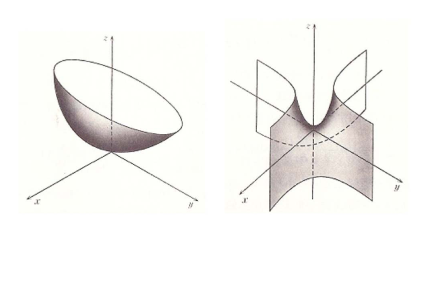
To account the exact meaning of intrinsicness of the Gaussian curvature, we consider another surface , and let be a one-to-one correspondence from to preserving the distance of two points and the angle between two directions (such is called an isometry in the present-day terms; see Sect. 20). If we would adopt the approach mentioned above on intrinsicness, Gauss’s outcome could be rephrased as “.” In particular, for a cylindrical surface , since , which is ostensibly curved, is deformed without distortion to a strip in the plane. This example articulately signifies that the Gaussian curvature could be possibly defined without the aid of the outside.
Executing lengthy computations, Gauss confirmed the intrinsicness of (see Sect. 17).646464Crucial in his argument is the commutativity of partial differentiation. Euler and A. C. Clairaut knew it, but the first correct proof was given by K. H. A. Schwarz in 1873. Since the goal is more than a pleasing astonishment, Gauss named his outcome “Theorema Egregium (remarkable theorem)” (Disquisitiones generales, Art. 12). Actually, it is no exaggeration to say that this theorem is a breakthrough not only in geometry, but also in cosmology. The following is his own words (1825) unfolded in a letter to the P. A. Hansen:
This research is deeply entwined with much else, I would like to say, with metaphysics of space and I find it difficult to shake off the consequences of this, such as for instance the true metaphysics of negative or imaginary quantities (Werke, XII, p. 8. See [3]).656565Even in the 18th century, there were a few who did not accept negative number. For example, F. Maseres said, “[negative numbers] darken the very whole doctrines of the equations and make dark of the things which are in their nature excessively obvious and simple” (1758). Although limited to the practical use, negative numbers already appeared in the Jiuzhang Suanshu (The Nine Chapters on the Mathematical Art) written in the period of the Han Dynasty (202 BCE–8 CE). The reason why the Chinese accepted negative numbers is, in all likelihood, that they had the concept of yin (negative or dark) and yang (positive or bright).
Although the Theorema Egregium has a deep metaphysical nature as Gauss put it, his incipient motivation came from the practical activity pertaining to the geodetic survey of Hanover to link up with the existing Danish grid that started in 1818 and continued for 8 years. He traveled across the state in order to cover the whole country. Fueled by this arduous activity, he brought out many papers on the geometry of curves and surfaces from about 1820 onwards. The Theorema Egregium is a culmination of his intensive study in this field.
Remark 7.2
In her study of elasticity (1831), M.-S. Germain introduced the mean curvature , which appears in a characterization of minimal surfaces; that is, the surface area of is locally minimized if and only if . Putting , we have and . The eigenvalues of are called the principal curvatures of . Obviously (Disquisitiones generales, Art. 8) and .
8 Number systems
It is off the subject, but while looking at the background behind Gauss’s opinion about complex numbers quoted above, we shall prepare some material related to what we shall describe later (Sect. 21).
Gerolamo Cardano (1501–1576), who stood out above the rest at that time as an algebraicist, acknowledged the existence of complex numbers in his Ars Magna (1545) that contains the first printed solutions to cubic and quartic equations. He observed that his formula may possibly involve complex numbers even when applied to a cubic equation possessing only real solutions.666666For example, his formula applied to the cubic equation yields a solution . Yet, he did not understand the nature of complex numbers and even thought that they are useless. Subsequently, Rafael Bombelli (1526–1572) took down the rules for multiplication of complex numbers (binomio) in his Book I of L’Algebra, while Descartes used the term “imaginary number” (nombre imaginaire) with the meaning of contempt. Wallis insisted that imaginary numbers are not unuseful and absurd when properly understood by using a geometric model just like negative numbers (Algebra, Vol. II, Chap. LXVI, 1673). Meanwhile, Euler persuaded himself that there is an advantage for the use of imaginary numbers (1751), and introduced the symbol for the imaginary unit (1755). It was around 1740 that he found the earth-shaking formula .
In 1799, Gauss gained his doctorate in absentia from the University of Helmstedt. The subject of his thesis is the fundamental theorem of algebra,676767Demonstratio nova theorematis omnem functionem algebraicam rationalem integram unius variabilis in factores reales primi vel secundi gradus resolvi posse. However, his proof had a gap. He gave three other proofs (1816, 1849) (see Sect. 21 for a “topological” proof). which, with a long history of inspiring many mathematicians, says that every polynomial equation with complex coefficients has at least one complex root.686868Albert Girard (1595–1632) was the first to suggest the fundamental theorem of algebra (FTA) (Invention Nouvelle en l’Algèbre, 1629). Meanwhile, Leibniz claimed that affords a counterexample for the FTA (1702). He assumed that the square root of should be a more complicated “imaginary” entity, not able to be expressed as ; but the truth is that (any double sign). Euler (1742) and D’Alembert (1746) counted on the FTA when they dealt with indefinite integrals of rational functions. As the title of his thesis indicates, he shied away from the use of imaginary numbers, notwithstanding that Gauss already had a tangible image. In a letter to F. W. Bessel, dated December 18, 1811, he communicated, “first I would like to ask anyone who wishes to introduce a new function into analysis to explain whether he wishes it to be applied merely to real quantities, and regard imaginary values of the argument only as an appendage, or whether he agrees with my thesis that in the realm of quantities the imaginaries have to be accorded equal rights with the reals. Here it is not a question of practical value; analysis is for me an independent science, which would suffer serious loss of beauty and completeness, and would have constantly to impose very tiresome restrictions on truths which would hold generally otherwise, if these imaginary quantities were to be neglected…” (Werke, X, p. 366–367; see [15]).
In 1833, William Rowan Hamilton (1805-1865) conceived the idea to express a complex number by the point in the coordinate plane ,696969Gauss had been in possession of the geometric representation of complex numbers since 1796. In 1797, C. Wessel presented a memoir to the Copenhagen Academy of Sciences in which he announced the same idea, but it did not attract attention. In 1806, J. R. Argand went public with the same formulation. which motivated him to construct 3D “numbers” with arithmetical operations similar to complex numbers, but the quest was a dead end. Alternatively, he discovered quaternions, the 4D numbers at the expense of commutativity of multiplication (1843). Specifically, the multiplication is defined by
| (8.1) |
In Hamilton’s notations, , , , so that quaternions are represented in the form: . A fact deserving special mention is that putting for , we have , the identity similar to for complex numbers, which agrees with the four-square identity discovered by Euler in 1748 during his investigation on sums of four squares (see Remark 14.1).
It may be said, incidentally, that Gauss had already discovered quaternions in 1818 (Mutationen des Raumes, Werke, VIII, 357–361). What he observed is, though his original expression is slightly different, that the rotation group is parameterized by with as
and . Note here that quaternions with form a group, which is identified with the spin group , pertinent to the quantum version of angular momentum that describes internal degrees of freedom of electrons. Additionally, the kernel of the homomorphism is a homomorphism of onto whose kernel is (Remark 21.1).
Remark 8.1
Euler discovered his formula while studying differential equations with constant coefficients (1748). Previously, de Moivre derived a formula that later brought on what we now call de Moivre’s theorem (1707), a precursor of Euler’s formula. Subsequently, R. Cotes had given the formula in 1714, but overlooked that the complex logarithm assumes infinitely many values, differing by multiples of , as found by Euler (1746).707070The logarithmic function originated from the computational demands of the late 16th century in observational astronomy, long-distance navigation, and geodesy. The main contributors are John Napier (1550–1617), Joost Bürgi, Henry Briggs, Oughtred, and Kepler. The term logarithm, literally “ratio-number” from λ´ογος and ὰριϑμ´ος, was coined by Napier in his pamphlet Mirifici Logarithmorum Canonis Descriptio (1614). Kepler studied Napier’s pamphlet in 1619, and published the logarithmic tables Chilias Logarithmoria (1624), which he used in his calculations of the Tabulae Rudolphinae Astronomicae (1627), a star catalog and planetary tables based on the observations of Tycho Brahe.
Before the problem of the complex logarithm was settled by Euler, there were arguments between Leibniz and Johann Bernoulli (1667–1748) in 1712 and then between Euler and Jean-Baptiste le Rond d’Alembert (1717–1783) around 1746 about for a negative . Leibniz says that does not exist, while Bernoulli alleges that . In the above-mentioned letter to Bessel in 1811, Gauss renewed the question about the multivaluedness of the complex logarithm, representing as the complex line integral , where is a curve in joining and (see Sect. 21). He further referred to what we now call Cauchy’s integral theorem.717171Augustin-Louis Cauchy defined complex line integrals in 1825 and established his theorem in 1851.
9 Euclid’s Elements
Gauss is one of the discoverers of non-Euclidean geometry (a geometry consistently built under the assumption that there are more than one line through a point which do not meet a given line), but he did not publish his work and only disclosed it in letters to his friends.727272For instance, his discovery was mentioned in a letter to F. A. Taurinus dated November 8, 1824 (Werke, VIII, p. 186). His hesitation in part came from the atmosphere in those days; that is, his new geometry was entirely against the predominant Kantianism. He wanted to avoid controversial issues,737373In a letter to Bessel dated January 27, 1829, Gauss writes, “I fear the cry of the Boetians [known as vulgarians] if I were to voice my views” (Werke, VIII, p. 200). and requested his friends not to make it public.
The other discoverers of the new geometry are Nikolai Ivanovich Lobachevsky (1792–1856) and János Bolyai (1802–1860).747474Strictly speaking, both Lobachevsky and Bolyai discovered the 3D geometry, while Gauss dealt only with the 2D case (Sect. 11). In 1826, Lobachevsky stated publicly that the new geometry exists.757575Lobachevsky, Exposition succincte des principes de la géométrie avec une démonstration rigoureuse du théorème des parallèles;O nachalakh geometrii, Kazanskii Vestnik, (1829–1830). Fourteen years later, as this research did not draw attention, he issued a small book in German containing a summary of his work to appeal to the mathematical community,767676Geometrischen Untersuchungen zur Theorie der Parallellinien (1840). and then put out his final work Pangéométrie ou précis de géométrie fondée sur une théorie générale et rigoureuse des parallèles, a year before his death (1855); see [17]. Meanwhile, in a break with tradition, Bolyai independently began his head-on approach to the non-Euclidean properties as early as 1823. In a letter to his father Farkas, on November 3, 1823, János says with confidence, “I discovered a whole new world out of nothing,” and made public his discovery in a 26-pages appendix Scientiam spatii absolute veram exhibens to his father’s book.777777 Tentamen juventutem studiosam in elementa Matheseos Purae (1832).
Gauss was a perfectionist by all accounts. He did not publish many outcomes, fearing that they were never perfect enough; his motto was “pauca sed matura—few, but ripe.” After his death it was discovered that many results credited to others had been already worked out by him (remember Cauchy’s integral theorem; Remark 8.1). The extraordinariness of Gauss may be narrated by the joke: Suppose you discovered something new. If Gauss would be still alive and would browse your result, then he would say, “Ah, that’s in my paper,” and surely would take an unpublished article out of a drawer in his desk. This was no joke for János Bolyai. Gauss received a copy of his father’s book in 1832, and endorsed the discovery in the response. To János’ disappointment, his cool reply reads, “The entire contents of your son’s work coincides almost exactly with my own meditation, which has occupied my mind for from thirty to thirty-five years” (Werke, VIII, p. 220). So much disappointed, János wholly withdrew from scientific activity, though Gauss wrote to Gerling (February 14, 1832), “I consider the young geometer Bolyai a genius of the first rank” (see [4]). As regards Lobachevsky, it was not until 1841 that his work was recognized by Gauss who looked over the Geometrischen Untersuchungen by chance. Gauss was very impressed with it, and praised Lobachevsky as a clever mathematician in a letter to his friend J. F. Encke (February 1841; Werke, VIII, p. 232).787878F. K. Schweikart, a professor of law and an uncle of Taurinus, had a germinal idea of non-Euclidean geometry (“astral geometry” in his term), and asked for Gauss, through Gerling, to comment on the idea in 1818. In response to the request (March 16, 1819), Gauss communicated, with compliments, that he concurred in Schweikart’s observation (Werke, VIII, p. 181). However Schweikart neither elaborated his idea nor published any result.
Now, what is known about Euclid and his Elements? It is popularly thought that Euclid was attached to Plato’s Academeia or at least was affiliated with it, and that he was temporarily a member of the Great Museum during the reign of Ptolemy I. Truth to tell, very little is known about his life. Archimedes, whose life, too, overlapped the reign of Ptolemy I, mentioned briefly Euclid in his On the Sphere and the Cylinder I.2, though being a fiction made by the posterity. In the Collection VII, Pappus records that Apollonius spent a long time with the disciples of Euclid in Alexandria. Apollonius himself referred to Euclid’s achievement with the statement that his method surpasses Euclid’s Conics. Proclus Diadochus (412 CE–485 CE) and Joannes Stobabeing (the 5th century CE) recorded the oft-told (but not trustworthy) anecdotes about Euclid. The sure thing is that he is the author of the definitive mathematical treatise Elements (Στοιχει̃α),797979Besides the Elements, at least five works of Euclid have survived to today; Data, On Divisions of Figures, Catoptrics, Phaenomena, Optics. There are a few other works that are attributed to Euclid but have been lost: Conics, Porisms, Pseudaria, Surface Loci, Mechanics. which is a crystallization of the plane and space geometry known in his day (ca. 300 BCE) and was so predominant that all earlier texts were driven out. It is solely to the Elements, one of the most influential books in long history, which Euclid owes his abiding fame in spite of his shadowy profile.
The Elements, consisting of thirteen books, starts with the construction of equilateral triangles and ends up with the classification of the regular solids; tetrahedron, cube, octahedron, dodecahedron, and icosahedron (Book XIII, Prop. 465). This suggests the influence of Pythagorean mysticism that put great emphasis on aesthetic issues, which, nowadays, are described in terms of symmetry (ςυμμετρία).808080“Symmetry” is explicated by group actions, with which both spatial homogeneity and isotropy are described. Klein’s Erlangen Program is also explained in this framework. Aetius (1st- or 2nd-century CE) says that Pythagoras discovered the five regular solids (De Placitis), while Proclus argues that it was the historical Theaetetus (ca. 417 BCE–ca. 369 BCE) who theoretically constructed the five solids. Plato’s Timaeus (53b5–6) provides the earliest known description of these solids as a group. Nowadays, regular polyhedra are discussed often in relation to finite subgroups (polyhedral groups) of or . For example, the icosahedral group is the rotational symmetry group of the icosahedron (see Remark 21.1). Moreover, it has an orderly organization consisting of 23 fundamental definitions, 5 postulates, 5 axioms, and 465 propositions. The “reductio ad absurdum” is made full use of as a powerful gambit (Prop. 6 in Book I is the first one proved by reductio ad absurdum).
As often said, only a few theorems are thought of having been discovered by Euclid himself. The theorem of angle-sum (Book I, Prop. 32), the Pythagorean Theorem (Book I, Prop. 47), and perhaps the triangle inequality (Book I, Prop. 20) are attributed to the Pythagoreans. The theory of proportions (Book V) and the method of exhaustion (Book X, Prop. 1, Book XII) are, as we mentioned before, greatly indebted to Eudoxus.
We shall talk about a checkered history of the Elements, originally written on fragile papyrus scrolls.818181In the tiny fragment “Papyrus Oxyrhynchus 29” housed in the library of the University of Pennsylvania, one can see a diagram related to Prop. 5 of Book II, which can be construed in modern terms as . The book survived in Alexandria and Byzantium under the control of the Roman Empire. In contrast, Roman people—the potentates of the world during this period—by and large expressed little interest in pure sciences as testified by Marcus Tullius Cicero (BCE 106–BCE 43), who confesses, “Among the Greeks, nothing was more glorious than mathematics. We, however, have limited the usability of this art to measuring and calculating” (Tusculanae Disputationes, ca. 45 BCE). Luckily, Alexandria is far away from the central government of the Empire, disintegrating in scandal and corruption. Situated as it was and thanks to the Hellenistic tradition, pure science flourished there. The people involved were Heron (ca. 10 CE–ca. 70 CE), Menelaus (ca. 70 CE–ca. 140 CE), Ptolemy, Diophantus (ca. 215 CE–ca. 285 CE), Pappus, Theon Alexandricus (ca. 335 CE–ca. 405 CE), and Hypatia (ca. 350 CE–415 CE).828282Diophantus stands out as unique because he applied himself to some algebraic problems in the time when geometry was still in the saddle. Theon is known for editing the Elements with commentaries. His version was the only Greek text known, until a hand-written copy of the Elements in the 10th century was discovered in the Vatican library (1808). Hypatia, a daughter of Theon, is the earliest female mathematician in history, and is far better known for her awful death; she was dragged to her death by fanatical Christian mobs.
But even in the glorious city, scientific attitude declined with the lapse of time, as the academic priority had been given, if anything, to annotations on predecessor’s work, and eventually fell into a state of decadence. This was paralleled by the steady decay of the city itself that all too often suffered overwhelming natural and manmade disasters. After a long tumultuous times, the great city was finally turned over to Muslim hands (641 CE).
In the Dark Ages, Europeans could no longer understand the Elements. In this circumstance, Anicius Manlius Boethius (ca. 480 CE–524 CE) and Flavius Magnus Aurelius Cassiodorus Senator (ca. 485 CE–ca. 585 CE) are very rare typical scholars in this period who were largely influential during the Middle Ages. Meanwhile, the Elements was brought from Byzantium to the Islamic world in ca. 760 CE, and was taught in Bagdad, Cordova, and Toledo where there were large-scale libraries comparable with the Great Museum in Alexandria.838383Worthy to mention is the House of Wisdom (Bayt al-Hikma) in Bagdad. It was founded by Caliph Harun al-Rashid (ca. 763 CE–809 CE) as an academic institute devoted to translations, research, and education, and was culminated under his son Caliph al-Mamoon. Al-Khwrizmī was a scholar at this institute.
After approximately 400 years of blank period in Europe, Adelard of Bath (Remark 2.1 (2)), who undertook a journey to Cordova around 1120 to delve into Arabic texts of Greek classics, obtained a copy of the book and translated it into Latin. Later on, Gerard (fn. 6) translated it into Latin from another Arabic version procured in Toledo. His translation is considered being close to the Greek original text. Then, in the mid-renaissance, only 27 years later from the type printing of the Bible by Johannes Gutenberg in Mainz, the first printed edition—based on the Latin version from the Arabic by Campanus of Novara who probably had access to Adelard’s translation—was published in Venice. Thereafter, versions of the Elements in various languages had been printed. The first English-language edition was printed in 1570 by H. Billingsley. Then in 1607, Matteo Ricci and Xu Guangqi translated into Chinese the first six volumes of the Latin version published in 1574 by Christopher Clavius.
One of the first multicolored books The First Six Books of the Elements of Euclid by O. Byrne was printed in 1847 in London. A. De Morgan was very critical of its non-traditional style embellished by pictorial proofs, and judged this inventive attempt to be nonsense (A Budget of Paradoxes, 1872). At that time, there was considerable debate about how to teach geometry; say, the pros and cons of whether to adopt a new approach to Euclidean geometry in teaching. C. Dodgson in Oxford, known as Lewis Carroll, assumed a critical attitude to his colleague Playfair who tried to simplify the Euclid’s proofs by introducing algebraic notations. In the little book Euclid and his Modern Rivals printed in 1879, he argues, “no sufficient reasons have yet been shown for abandoning [Euclid’s Elements] in favour of any one of the modern Manuals which have been offered as substitutes.” G. B. Halsted says, in the translator’s introduction to J. Bolyai’s Scientiam spatii, “Even today (1895), in the vast system of examinations carried out by the British Government, by Oxford, and by Cambridge, no proof of a theorem in geometry will be accepted which infringes Euclid’s sequence of propositions.” As a matter of course, it is now seldom to make direct use of Euclid’s propositions for university examinations, but the book went through more than 2000 editions to date, and has been (and still is) the encouragement and guide of scientific thought. Furthermore, modern mathematics inherits much of its style from the Elements; in particular, many mathematical theories, even if not all of them, begin with axiomatic systems (Sect. 18).
What about the original Greek text? It was Heiberg (fn. 12) who tracked down all extant manuscripts—the aforementioned Greek Vatican manuscript is one of them—to produce a definitive Greek text together with its Latin translation and prolegomena (Euclidis Opera Omnia, 8 vols, 1883–1916). This is a trailblazing achievement that has become the basis of later researches on Euclid.
10 The Fifth Postulate
Euclid’s greatest contribution is his daring selection of a few postulates as major premises (if not completely adequate from today’s view), of which Greek geometers thought as self-evident truth requiring no proof. He built up a deductive system in which every theorem is derived from these postulates. Among his five postulates, the last one, called the Fifth Postulate (FP henceforward), constitutes the core of our story on non-Euclidean geometry. It says:
If a straight line falls on two straight lines in such a manner that the interior angles on the same side are together less than two right angles, then the straight lines, if produced indefinitely, meet on that side on which are the angles less than the two right angles ([7], Book I).
The theorem of angle-sum and the Pythagorean Theorem rely on this postulate. For example, what is required for the former is the fact that “if a straight line fall upon two parallel straight lines it will make the alternate angles equal to one another” (Prop. 29 in Book I), which is a consequence of the FP.848484In contrast to these two theorems, the triangle inequality is proved without invoking the FP (Book I, Prop. 20).
The first four postulates have fairly simple forms; say, the first one declares, in today’s terms, that given two points, there exists a straight line through these points, whereas the necessity of the last postulate is by no means overt, owing not only to the intricacy of its formulation, but also to the fact that the converse of Prop. 29 is proved without an appeal to the last postulate (Prop. 27). Actually the last one had been believed to be redundant and hence to be a “proposition” all through modern times until the second decade of the 19th century ([2]).
An elaborate and stalwart attempt to vindicate Euclidean geometry by “proving” the FP was done by Girolamo Saccheri (1667-1733), an Italian Jesuit priest, who explored the consequences under the negation of the postulate, hoping to reach a contradiction. For this sake, he made use of quadrilaterals of which two opposite sides are equal to each other and perpendicular to the base, and set up the following three hypotheses (Fig. 8);858585Omar Khayyam (1048–1131) dealt with the FP in his Explanation of the Difficulties in the Postulates of Euclid. He is considered a predecessor of Saccheri.
(i) the hypothesis of the right angle: ,
(ii) the hypothesis of the obtuse angle: , and
(iii) the hypothesis of the acute angle: ,
where the first hypothesis is equivalent to the FP. Examining these hypotheses meticulously, he concluded that hypothesis (ii) contradicts the infinite extent of plane, and is false, but could not exclude hypothesis (iii). At the final stage of his argument, Saccheri appeals to intuition about our space, and says, “Hypothesis anguli acuti est absolute falsa; quia repugnans naturae liniae rectae” [“the hypothesis of the acute angle is absolutely false; because it is repugnant to the nature of the straight line”] ([2]). In summary, he virtually proved that, under the negation of the FP, the angle-sum of any triangle is less than (thus the existence of a triangle with angle-sum of implies the FP).868686Saccheri, Euclides ab omni naevo vindicatus sive conatus geometricus quo stabiliuntur prima ipsa geometriae principia (1733). See [32].
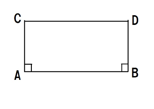
Johann Heinrich Lambert (1728–1777)—conceivably familiar with Saccheri’s work because, in his Theorie der Parallellinien (1766), he quoted the work of G. S. Klügel who listed nearly 30 attempts to prove the FP including Saccheri’s work878787Conatuum praecipuorum theoriam parallelarum demonstrandi recensio (1763).—investigated the FP in alignment with an idea resembling that of Saccheri ([2], p. 44).888888Lambert proved that the transfer time from to along a Keplerian orbit is independent of the orbit’s eccentricity and depends only on and (Über die Eigenschaften der Kometenbewegung, 1761). He was the first to express Newton’s second law of motion in the notation of differential calculus (Vis Viva, 1783). His work, published after the author’s death, bristles with far-sighted observations and highly speculative remarks (see [26]). One of his revelations is that, under the negation of the FP, the angular defect for a triangle is proportional to the area of the triangle. This is inferred from the fact that if we define for a polygon with sides by setting , then and the area functional share the “additive property”; i.e., for a polygon composed of two polygons , . With this observation in hand, he ratiocinated that non-Euclidean plane-geometry (if it exists) has a close resemblance to spherical geometry.
Let us briefly touch on spherical geometry, which is nearly as old as Euclidean geometry, and was developed in connection with geography and astronomy. In his Sphaerica, extant only in an Arabic translation, Menelaus introduced the notion of spherical triangle, a figure formed on a sphere by three great circular arcs intersecting pairwise in three vertices. He observed that the angle-sum of a spherical triangle is greater than ([28]). Greek spherical geometry gave birth to spherical trigonometry that deals with the relations between trigonometric functions of the sides and angles of spherical triangles. At a later time, it was treated in Islamic mathematics and then by Viète, Napier, and others. A culmination is the following fundamental formulas given by Euler.898989Trigonometria sphaerica universa, ex primis principiis breviter et dilucide derivata, Acta Academiae Scientarum Imperialis Petropolitinae, 3 (1782), 72–86 (see [25]). The spherical cosine law (10.2) is seen in al-Battnī’s work Kitb az-Zīj (fn. 21).
| (10.1) | ||||
| (10.2) |
where is a spherical triangle on the sphere of radius , and are the arc-length of the edges corresponding to , respectively.
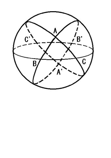
Now, what Lambert paid attention to is the formula , a refinement of Menelaus’ observation on spherical triangles discovered by Harriot (1603) and Girard (Invention nouvelle en algebra, 1629), and probably known by Regiomontanus.909090The Latin name of Johannes Müller von Königsberg (1436–1476), the most important astronomer of the 15th century who may have arrived at the heliocentricism. Replacing the radius by in this formula, we obtain , which fits in with his outcome on the angular defect, and brought him to the speculation that an “imaginary sphere” (under a suitable justification) provides a model of “non-Euclidean plane,” but he did not pursue this idea any further.
Remark 10.1
(1) Here is a list (by no means exhaustive) of people who tried to deduce the FP from other propositions: Posidonius of Apameia (ca. 135 BCE–ca. 51 BCE), Geminus of Rhodes (the 1st century BCE), Ptolemy, Proclus, Nasīr al-Dīn Tsī(1201–1274), C. Clavius (1538–1612), P. A. Cataldi (1548–1626), G. A. Borelli (1608–1679), G. Vitale (1633–1711), Leibniz, Wallis, J. S. König (1712–1757), Adrien-Marie Legendre (1752–1833), B. F. Thibaut (1775–1832), and F. Bolyai. Gauss, J. Bolyai, and Lobachevsky were, for that matter, no exception at the beginning of their studies of parallels. What is in common to their arguments (except for the great trio) is that they beg the question; that is, they assume what they intend to prove.
(2) The system of postulates in the Elements is not complete. An airtight system was provided by Hilbert in the text Grundlagen der Geometrie (1899). His system consists of five main axioms; I. Axioms of Incidence, II. Axioms of Order, III. Axioms of Congruence, IV. Axiom of Parallels, V. Axioms of Continuity.919191 Moritz Pasch (1843–1930), Giuseppe Peano (1858–1932), and Mario Pieri (1860–1913) contributed to the axiomatic foundation of Euclidean geometry. The Axiom of Parallels says, “Given a line and a point outside it, there is exactly one line through the given point which lies in the plane of the given line and point so that the two lines do not meet.” This statement, clearly given by Proclus in his commentary, was adopted by Playfair in his edition of the Elements (1795) as an alternative for the FP. Hilbert’s Axioms of Continuity consists of the axiom of completeness related to Dedekind cuts (Remark 4.2 (4)) and the Axiom of Archimedes.
11 Discovery of non-Euclidean geometry
We now go back to Gauss’s discovery of non-Euclidean geometry. In his letter to Taurinus in 1824, Gauss mentions, “The assumption that angle-sum [of triangle] is less than leads to a curious geometry, quite different from ours [the euclidean] but thoroughly consistent, which I have developed to my entire satisfaction. The theorems of this geometry appear to be paradoxical, and, to the uninitiated, absurd, but calm, steady reflection reveals that they contain nothing at all impossible” (see [1]).
Now, when did Gauss become aware of the new geometry? A few tantalizing pieces of evidence are in Gauss’s Mathematisches Tagebuch, a record of his discoveries from 1796 to 1814 (Werke, X).929292Gauss’s diary—which contains 146 entries written down from time to time, and most of which consist of brief and somewhat cryptical statements—was kept by his bereaved until 1899. The 80th entry (October, 1797) announces the discovery of the proof of the FTA. The 72nd item written on July 28, 1797 says, “Plani possibilitatem demostravi” [“I have demonstrated the possibility of a plane”]. This seems to indicate Gauss’s interest in the foundation of Euclidean geometry, of which he never lost sight from that time onward. Following that, in the 99th entry dated September 1799, he wrote, “In principiis Geometriae egregios progressus fecimus” [“On the foundation of geometry, I could make a remarkable progress”]. It is difficult to imagine what this oblique statement means, but it could have something to do with non-Euclidean geometry.939393In a letter to F. Bolyai, March 6, 1832 (Werke VIII, p. 224), Gauss alluded that Kant was wrong in asserting that space is only the form of our intuition. In the same year, Gauss confided to F. Bolyai to the effect that he had doubt about the truth of geometry.949494In the letter, he also said, “If one could prove the existence of a triangle of arbitrarily great area, all Euclidean geometry would be validated” (see [4]). However, his letter to F. Bolyai in 1804 witnessed that he was still suspicious of the new geometry (Werke, VIII, p. 160). All of the available witnesses point to the possibility that it is in 1817 at the latest that Gauss disengaged himself from his preconceptions, and began to deal seriously with the new geometry. In a letter to his friend H. Olbers (April 28, 1817), he elusively says, “I am becoming more and more convinced that the necessity of our geometry cannot be proved” (Werke, VIII, p. 177).
In all likelihood, Gauss had a project to bring out an exposition of the “Nicht-Euklidische Geometrie”. His unpublished notes about the new theory of parallels might be part of this exposition (Werke, VIII, p. 202–209). A letter addressed to Schumacher on May 17, 1831 says, “In the last few weeks, I have begun to write up a few of my own meditations, which in part are already about 40 years old.”959595In a letter to Schumacher of July 12, 1831, Gauss said that the circumference of a non-Euclidean circle of radius is where is a positive constant (Werke, VIII, p. 215), which turns out to coincide with the radius of the imaginary sphere. His project was, however, suspended upon the receipt of a copy of J. Bolyai’s work. Accordingly, the detailed study of the new geometry was put in the hands of Bolyai and Lobachevsky, who established, under the negation of the FP, an analogue of trigonometry, with which they could be confident of the consistency of the new geometry ([17] and [24]).
The fundamental formulas in non-Euclidean trigonometry are given by
| (11.1) | |||
| (11.2) |
These are obtained from the trigonometric formulas established by Bolyai and Lobachevsky.969696The non-Euclidean formulas were found by Taurinus (Geometriae Prima Elementa, 1826), but the outcome did not wholly convince him of the possibility of a new geometry. Notice here that, thanks to Euler’s formula, we get (11.1) and (11.2) by transforming into in (10.1) and (10.2), thereby justifying Lambert’s anticipation of a new geometry on the imaginary sphere.
We should underline here that non-Euclidean geometry involves a positive parameter just like spherical geometry involving the radius of a sphere. As Lambert took notice of it, this implies that, once is selected, the absolute unit of length is determined.979797In the ordinary geometry, only a relative meaning is attached to the choice of a particular unit in the measurement. The concept of “similarity” arises exactly from this fact. Actually, the non-existence of an absolute unit of length is equivalent to the FP. Failing to notice this fact, Legendre believed that he succeeded in proving the FP.989898Léflexions sur différentes manières de démontrer la théorie des paralléles ou le théorème sur la somme des trois angles du triangle, 1833. In his futile attempt to prove the FP, Legendre rediscovered Saccheri’s result. The error in his “proof” was pointed out by Gauss in a letter to Gerling (1816; Werke, VIII, p.168, 175). (By 1808, Gauss realized that the new geometry must have an absolute unit of length; Werke VIII, p.165.)
Thus the issue of the FP, which had perplexed many able scholars for more than 2000 years, was almost settled down (the reason why we say “almost” will become clear later). More than that, mathematicians grew to realize that postulates in general are not statements which are regarded as being established, accepted, or self-evidently true, but a sort of predefined rules.
On reflection, Euclid’s choice of the FP shows his keen insight and deserves great veneration. Thomas Little Heath (1861–1940), a leading authority of Greek mathematics, remarked that “when we consider the countless successive attempts made through more than twenty centuries to prove the Postulate, many of them by geometers of ability, we cannot but admire the genius of the man who concluded that such a hypothesis, which he found necessary to the validity of his whole system of geometry, was really indemonstrable” ([7], p. 202).
12 Geodesics
In Sect. 7, we stressed the role of shortest curves in the intrinsic measurement in a surface. In order to outline another work of Gauss related to non-Euclidean geometry, we shall take a look at such curves from a general point of view.
The length of a curve , , on a surface is given by . Thus our issue boils down to finding a curve that minimizes among all curves on satisfying the boundary condition , . Johann Bernoulli raised the problem of the shortest distance between two points on a convex surface (1697). Following his senescent teacher Johann, Euler obtained a differential equation for shortest curves on a surface given by an equation of the form (1732).
Finding shortest curves is a quintessential problem in the calculus of variations, a central plank of mathematical analysis originated by Euler, which deals with maximizing or minimizing a general functional (i.e., a function whose “variable” is functions or maps). A bud of this newly-born field is glimpsed in Fermat’s principle of least time, but the derivation of Snell’s law is a straightforward application of the usual extreme value problem. The starting point in effect was the brachistochrone curve problem raised by Johann Bernoulli (1696);999999“Brachistochrone” is from the Greek words βράχιςτος (shortest) and χρ´ονος (time). The first to consider the brachistochrone problem is Galileo (Two New Sciences). the problem of finding the shape of the curve down which a sliding particle, starting at rest from and accelerated by gravity, will slip (without friction) to a given point in the least time. To be exact, the problem is to find a function which minimizes the integral .
In the paper Elementa Calculi Variationum read to the Berlin Academy on September 16, 1756, Euler unified various variational problems. At about the same time, Joseph-Louis Lagrange (1736–1813) simplified Euler’s earlier analysis and derived what we now call the Euler-Lagrange equation (E-L equation). Especially, his letter to Euler dated August 12, 1755 (when he was only 19 years old!) contains the technique used today. Here in general (however restricted to the case of one-variable), the E-L equation associated with the functional of the form
| (12.1) |
is given by
| (12.2) |
What Lagrange proved is that minimizing is a solution of (12.2).
Applying the E-L equation to length-minimizing curves on a surface, we obtain an ordinary differential equation for . What should be aware of is that a solution of this equation is only a locally length-minimizing curve; not necessarily shortest. Such a curve is called a geodesic, the term (coming from geodesy) coined by Joseph Liouville (1809–1882).100100100De la ligne géodésique sur un ellipsoide quelconque, J. Math. Pures Appl., 9 (1844), 401–408. Strictly speaking, as a parameter of a geodesic, we adopt the one proportional to arc-length. We should note that is left invariant under a parameter change.
A geodesic may be defined as a trajectory of force-free motion. To explain this, we regard a curve in a surface as the trajectory of a particle in motion. The velocity vector is a vector tangent to at , but the acceleration vector is not necessarily tangent to . If the constraint force confining the particle to is the only force, then must be perpendicular to the tangent plane of at because the constraint force always acts vertically on . Such a curve turns out to be a geodesic. Hence, if we denote by the tangential part of , then is a geodesic if and only if . Since this is a second-order ordinary differential equation (see (17.5) and Sect. 20), we have a unique geodesic defined on an interval containing such that , for given a point and a vector tangent to at .
There is an alternative derivation of the equation , based on the principle of least action that was enunciated by Pierre Louis Moreau de Maupertuis (1698–1759) and occupies its position in the physicist’s pantheon,101101101Accord de différentes loix de la nature qui avoient jusqu’ici paru incompatibles, read to the French Academy on April 15, 1744. His paper Loi du repos des corps, Histoire Acad. R. Sci. Paris (1740), 170–176, is its forerunner. according to which a particle travels by the action-minimizing path between two points. The action he defined is the “sum of ” along the entire trajectory of a particle with mass , where is the length of a tiny segment on which the velocity of the particle is .102102102On reflection, the principle of least action seems to tell us that present events are dependent on later events in a certain manner; so, though a bit exaggerated, a natural occurrence seems to be founded on an intention directed to a certain end. For such a teleological and purposive flavor (dating back to Aristotle), Maupertuis thought that his cardinal principle proves a rational order in nature, and buttresses the existence of a rational God.
The obscurity of Maupertuis’ formulation was removed by Euler (1744)and Lagrange (1760). Specifically the action integral applied to a particle in motion under a given potential energy (the concept conceived by Lagrange in 1773) is: . The E-L equation for reduces to the Newtonian equation: . (For example, the gravitational potential energy generated by the mass distribution is .) This suggests us to define the action integral for a curve in by . Indeed, the E-L equation for this functional coincide with .
The minimum (maximum) problems come up in various scenes in geometry. For instance, the (classical) isoperimetric theorem whose origin goes back to ancient Greece states, “Among all planar regions with a given perimeter, the circle encloses the greatest area.” Needless to say, minimal surfaces are solutions of a minimum problem. In particular, finding a surface of the smallest area with a fixed bounday curve is known as Plateau’s problem, the problem raised by Lagrange in 1760 and investigated in depth in the 20th century onward.103103103 Plateau conducted experiments with soap films to study their configurations (1849). Minimum/maximum principles hold emphatic importance even in different fields; say, in potential theory (Remark 15.1 (1)), in statistical mechanics, in information science, in the design of crystal structures ([38]), and much else besides. Even more surprisingly, so too does in the characterization of the “shape” of the universe as will be explained later.
Remark 12.1
(1) Hamilton reformulated the E-L equation in the context of mechanics as follows (1835). For simplicity, suppose that the integrand in (12.1) (called a Lagrangian) does not involve the time variable . Making the change of variables where , and defining the function (the Hamiltonian) with the new variables by , we may transform (12.2) into what we call the Hamiltonian equation:
A general form of the law of the conservation of energy is then embodied by the fact that is constant for any solution . In the case where , we have and . Hence in this case is the momentum, and is the total mechanical energy; that is, the sum of the kinetic energy and the potential energy. Hamilton’s formulation gained further prominence with the advent of statistical mechanics and quantum mechanics.
(2) To outline a maximum principle in statistical mechanics, consider a simple quantum mechanical system with possible microscopic states whose energies are .104104104A quantum mechanical system is described by a self-adjoint operator acting on a Hilbert space. A unit eigenvector of with eigenvalue represents a state with energy . A (macroscopic) state of the system is described by a probability distribution , where is the probability that the microscopic state occurs during the system’s fluctuations. In this setting, the internal energy and the entropy are defined by , respectively, where is Boltzmann’s constant. Among all states with , there is a unique with the maximum entropy; i.e. . It is given by the Gibbs distribution105105105The term “entropy,” from Greek εν (“in”) + τροπή (“a turning”), was coined in the early 1850s by R. J. E. Clausius. In the 1870s, L. Boltzmann gave its statistical definition. representing the equilibrium state , where is the temperature, determined by the equation .
The second law of thermodynamics (formulated by Clausius) says that entropy of an isolated system invariably increases because the system evolves towards equilibrium. Therefore the total entropy of the universe is continually increasing.
13 Curvature and non-Euclidean geometry
In a nutshell, what Gauss discovered during his study of the new geometry is that homogeneity and isotropy are not enough to characterize Euclidean space; namely, his discovery suggests that there is another “space” with these properties, which is to be called “non-Euclidean space”. However, we have to stress that the way Gauss and others searched for their new geometry was synthetic. At this stage, therefore, the “new space” has not yet been explicitly described.
Gauss did not refer to the non-Euclidean space, but perhaps he was aware that the “new space” may yield an alternative model of the universe. In truth, the moment when he perceived this is by far the most significant turning point in cosmology.106106106In the Disquisitiones generales (Art. 28), Gauss refers to the numerical data for the triangle formed by the three mountain peaks Brocken, Hohenhagen, and Inselsberg. Some say that with these data Gauss wished to determine whether the universe is Euclidean. What we can say at the very least is that he compared a geodesic triangle on the earth surface with a plane rectilinear triangle. Meanwhile, Lobachevsky attempted to measure the angle sum of a triangle by analyzing data on the parallax of stars (Exposition succincte; see [19]). What is more, Gauss seemed to know an intimate relation between his intrinsic theory of surfaces and non-Euclidean (plane) geometry because he obtaind the arresting formula (Disquisitiones generales, Art. 20):
| (13.1) |
where is a geodesic triangle (a triangle on formed by the arcs of three geodesics segments; Fig. 10), and is the surface element of (Sect. 15). Note that this is a generalization of Harriot-Girard’s formula.
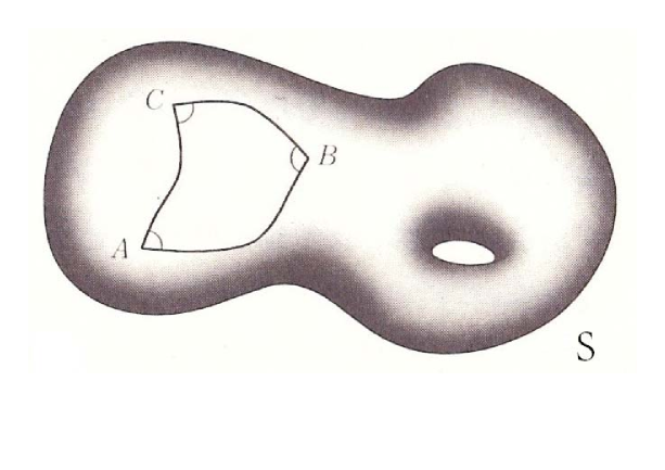
From (13.1), a “plane-like surface” of constant negative curvature (if exists) is expected to be a non-Euclidean plane-model, and hence finding such a surface became an urgent issue. In a note dated about 1827, Gauss jotted down his study about the surface of revolution generated by the tractrix (Fig. 11),107107107The tractrix is the graph of the function , which shows up as a locus of an object obtained from dragging it along a line with an inextensible string. The architect C. Perrault proposed a problem related to the tractrix (1670) for the first time. The appellation “tractrix” was coinded by Huygens in 1692. which he called “das Gegenstück der Kugel” (the opposite of the sphere).108108108This was to be called the pseudosphere by Eugenio Beltrami (1835–1900); see fn. 126. This is an example of a surface with constant negative curvature, but he did not mention clearly that it has to do with the new geometry (Werke, VIII, p. 265).109109109F. Minding found that the trigonometry for geodesic triangles on this surface enjoys analogy to spherical trigonometry (1840). However he did not notice that his finding is equivalent to the non-Euclidean trigonometric relations. The reason might be because he could not construct such a surface with a planar shape. The truth is that the non-Euclidean plane cannot be realized as an ordinary surface in space as Hilbert showed in 1901. In order to apprehend its true identity, we need the notion of manifold (Sect. 16).
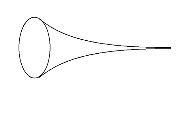
Gauss may have known (13.1) as early as 1816, so it may have served as a forerunner to the Theorema Egregium. In his Disquisitiones generales, Art. 20, he says, “This formula, if I am not wrong, should be counted among the most elegant ones of the theory of surfaces.”
Behind (13.1), there seems to be his commitment to electromagnetism;110110110The rapid progress of electromagnetism originated with H. C. Oersted who verified by experiment that electricity and magnetism are not independent (1820). in 1813, he proved a special case of what we call now Gauss’s flux law that correlates the distribution of electric charge with the resulting electric field. The law is expressed by a formula connecting an integral inside a closed surface with a surface integral over the boundary (divergence theorem; Werke, V, p. 5–7).
Remark 13.1
The divergence theorem asserts that
for a vector field defined on a domain with boundary , where is the outer unit normal of the surface . A special case was treated by Lagrange (1762), and by Gauss (1813). It was M. V. Ostrogradsky who gave the first proof for the general case (1826). The 2D version is known as Green’s theorem (1828):
| (13.2) |
where is the domain surrounded by a piecewise smooth, simple closed counterclockwise oriented curve . Another important formula is Stokes’ formula for a bordered surface with a normal unit vector field :
where we represent the boundary curve of by an arc-length parameterization in such a way that points towards the interior of .111111111The statement of Stokes’ formula appeared as a postscript to a letter (July 2, 1850) from William Thomson (Lord Kelvin, 1824–1907) to G. Stokes. Stokes set the theorem as a question on the 1854 Smith’s Prize Examination at Cambridge.
A formula that deserves to be mentioned is derived from (13.1).For a closed surface with a division by a collection of geodesic triangles such that each triangle side is entirely shared by two adjacent triangles, we have
| (13.3) |
where are the number of vertices, edges, and faces, respectively. This formula, due to Walther Franz Anton von Dyck (1856–1934), is called the Gauss-Bonnet formula, though they never referred to (13.3) in their work.112112112von Dyck, Beiträge zur Analysis situs I. Aufsatz. Ein- und zweidimensionale Mannigfaltigkeiten, Math. Ann., 32 (1888), 457–512. Pierre Ossian Bonnet (1819–1892) generalized (13.1) to triangles with non-geodesic sides (1848). It tells us that (the Euler characteristic of ) is independent of the choice of a triangulation. In particular, applying to the unit sphere , we get the polyhedron formula discovered by Euler in 1750 (Sect. 21).
The proof of (13.3) goes as follows. The sum of the interior angles gathering at each vertex is , so that
while because each edge is counted twice when we count edges of all triangles. Consequently, the left-hand side of (13.3) is equal to , as desired.
The Gauss-Bonnet formula opened the doorway to global analysis that knits together three fields; differential geometry, topology, and analysis (Sect. 21).
After Gauss’s monumental feat, cosmology began to remove itself from religion and even philosophy, and to snuggle up to higher mathematics which is unconstrained by perceptual experience; thus God walked away from the center stage. However the outside of space still remains as a backdrop. It was Riemann, the next protagonist in our story, who at last erased the outside.
14 The dimension of space
Deferring the account of Riemann’s achievement to the next section, we shall pause for a moment to discuss higher-dimensional spaces.
Dimension is, in a naive sense, a measurable extent of a particular kind, such as length, breadth and depth, or the maximum number of independent directions in a refined sense. Physically it is the number of degrees of freedom available for movement in a space. Aristotle was among the earliest who contemplated dimension; he says, “magnitude which is continuous in one dimension is length; in two breadth, in three depth, and there is no magnitude besides these” (Metaphysics, V, 11-14). Ptolemy likewise asserted in his book On Distance that one cannot consider “space of dimension more than three,” and even gave its proof as testified by Simplicius of Cilicia (ca. 490 CE–ca. 560 CE).
In Sect. 7, we speculated what the inhabitants in a surface would do when they want to know the shape of their universe. Surfaces are 2D, whilst our universe is 3D. Why are we in the 3D space, not in another?113113113Closely related to this question is the anthropic principle (Brandon Carter, 1973), the philosophical deliberation that the universe is inseparable from mankind’s very existence. However difficult it may have been to furnish a definite answer to this question, there is no barrier to thinking of higher-dimensional models of space. Actually we have a clue in analytic geometry to formulate coordinate spaces of general dimension.114114114Analytic geometry acquired its whole range in the 18th century with A. Parent, Clairaut, Euler, G. Cramer, Lagrange and many others. La Hire’s work Nouveaux élémens des sections coniques, les lieu géométriques (1679) summarized the progress of analytic geometry during a few decades since Descartes. His work contains some ideas leading to the extension of space to more than three dimensions.
It was in the 18th century that mathematicians began to contemplate the possibility of the use of as a gadget to develop mechanics. As Lagrange and D’Alembert suggested, it is natural to add the time parameter as the fourth dimension. Moreover, it is technically convenient to describe a mass system of particles located at as the single point in . Then, around the 1830s, the theory of -ple integrals was evolved. For instance, Carl Gustav Jacob Jacobi (1804–1851) computed the volume of a higher-dimensional sphere in connection with quadratic forms though he deliberately avoided geometrical language (1834).
Certain it is that, by the early 19th century, the time was ripe for developing higher-dimensional geometry. In 1843, Arthur Cayley published a small memoir on , however the paper is characteristically algebraic. In the same year, Hamilton conceived the 4D number system (Sect. 7). A year later, Die Lineale Ausdehnungslehre, ein neuer Zweig der Mathematik, a pioneer work on vector spaces of general dimension, was published by Hermann Grassmann (1809–1877).115115115In this book, he created what we now call the exterior algebra (or Grassmann algebra), which, denigrated at the time, was to exert a profound influence on the formation of algebra and geometry; see Sect. 20. In this sense, he was quite ahead of his time.
A point at issue is how to imagine as a higher-dimensional analogue of plane and space. A lighthearted way is to execute a geometry in by mimicking geometry in and (thus geometric terminology may be of psychological assistance when we imagine ). It is to the credit of Ludwig Schläfli (1814–1895) to have inaugurated the study of the geometry of along this line. In his magnum opus, Theorie der vielfachen Kontinuität, worked out from 1850 to 1852,116116116It was in 1901, after his death, that the entire manuscript was published in Denkschriften Der Schweizerischen Naturforschenden Gesellschaft, 38 (1901), 1–237. Schläfli defined the distance between and in by .
As expected, many results in are just direct generalizations of the facts that hold in plane and space, but there are several results depending heavily on dimension. Schläfli’s classification of higher-dimensional convex regular polytopes is such an example. Specifically, there are six regular polytopes in , while there are only three regular polytopes in , (the analogues of the tetrahedron, the cube and the octahedron). Another dimension-dependent example—rather recent one originating with Newton’s curiosity regarding celestial bodies—is the maximum possible kissing number for , where the kissing number is the number of non-overlapping unit spheres that can be arranged in such a way that each of them touches another given unit sphere. For example, , and , but curiously is unknown for except for and .117117117The fact was conjectured by Newton, while D. Gregory, a nephew of James Gregory, insisted that in a discussion taking place at Cambridge in 1694. A proof in favor of Newton was given by K. Schütte and van der Waerden (1953). Such phenomena enrich geometry; thereby, as opposed to Kant’s dictum, higher-dimensional geometry turns out to be non-empty and fruitful.
Remark 14.1
As mentioned in Sect. 7, there exists no 3D number system that inherits, in part, the arithmetic properties of real numbers, while a 4D system exists. Hence a dimension-dependence phenomenon occurs in number systems. In 1843, J. T. Graves discovered the octonions, a non-associative 8D number system, inspired by Hamilton’s discovery of quaternions.118118118Slightly before the publication of his paper, Cayley discovered the octonions. Octonions are often referred to as Cayley numbers. We thus have four number systems. These systems share the following properties; writing for multiplication of , we have , , and . Here . Interestingly, if has multiplication having these properties, then must be 1,2,4, or 8 as A. Hurwitz showed in 1898.
Quaternions and octonions—the products of pure thought— have applications in modern physics; thus being more than mathematical fabrications.
15 Riemann –The universe as a manifold
Gauss brought about a revolution in geometry as he envisaged. Indeed, his study of surfaces turned out to be the germ of a “science of generalized spaces” that was essentially embodied by Georg Friedrich Bernhard Riemann (1826–1866) in his Habilitationsschrift Über die Hypothesen welche der Geometrie zu Grunde liegen presented to the Council of Göttingen University.119119119Habilitationsschrift is a postdoctoral thesis required for qualification as a lecturer. This is his second stage of the procedure (see fn. 158 for his thesis at the first stage). The title of Riemann’s thesis is an implicit criticism of Kant.
It was Gauss—only one year before the death at the age of 78—who asked his brilliant disciple to prepare a thesis on the foundations of geometry, out of the three possible topics that Riemann proposed. The two other topics were on electrical theory, and unlike the one chosen by his mentor, he was well-prepared for them. So Riemann had to work out the topic Gauss recommended, and in a matter of months he could bring it to completion without qualm.
The aged Gauss, albeit being sick at that time, attended Riemann’s probationary lecture delivered on 10 June 1854 in anticipation of hearing something new related to his old work. “Among Riemann’s audience, only Gauss was able to appreciate the depth of Riemann’s thoughts. … The lecture exceeded all his expectations and greatly surprised him. Returning to the faculty meeting, he spoke with the greatest praise and rare enthusiasm to W. Weber about the depth of the thoughts that Riemann had presented” ([19]).
In his lecture aimed to a largely non-mathematical audience, Riemann posed profound questions about how geometry is connected to the world we live in. The thrust being as such, the content was much more philosophical than mathematical though he humbly denied this (Part I).
At the outset, he says that the traditional geometry assumes the notion of space and some premises which are merely nominal, while the relation of these assumptions remains in darkness because the general notion of multiply extended magnitude remained entirely unworked. He thus sets himself the task of constructing the notion of manifold of general dimension.
There is something of note here. In his setup, Riemann does not set a limit to the dimension of space. Remember that, when he inaugurated his study, higher-dimensional geometry as an abstract theory was just formulated. This might be a precipitating factor for his commitment to higher-dimensional curved spaces. His general treatment of space was, however, not a mere idea or pipe dream, and had truly a decisive influence on modern cosmology that employs manifolds of dimension more than four (in superstring theory, space-time is 10D).
Riemann continues his deliberation on manifolds, which is bolstered by his immense insight into the principles behind the proper understanding of our space; but to go straight to the heart of his scheme, let us take a shortcut at the expense of his true motive.
To single out a reasonable model of the universe, we must take into account the fact that our universe looks Euclidean in so far as we examine our vicinity. In the light of this observation, we define a -dimensional manifold to be a “generalized space” on which one can set up a curvilinear coordinate system around each point , so that we may indicate each point near by its coordinates . In addition, the higher-dimensional Pythagorean Theorem is supposed to hold in the infinitesimal sense. To explore what this means, we recall that the distance between and its displacement in is given by . When a skew coordinate system is taken instead of the Cartesian one, this expression is modified as . Here if the coordinate transformation between and is given by , then , and hence . The square matrix is a positive symmetric matrix. Since in the infinitesimally small scale, the curvilinear coordinate system is regarded as a skew coordinate system, it is natural to express the “infinitesimal” Pythagorean Theorem as
| (15.1) |
where the “line element” stands for the “distance between infinitesimally nearby points” and , and is, in turn, a function of the variables with values in positive symmetric matrices. The right-hand side is called the first fundamental form (or Riemannian metric in today’s term; Sect. 20), which is literally fundamental in Riemann’s theory of manifolds. With it, one can calculate the length of a curve by the integral
| (15.2) |
In imitation of the case of surfaces, we say that is a geodesic if it is locally length-minimizing. The distance of two points is defined to be the infimum of the length of curves joining .
The next task—a highlight of his thesis—is to define “curvature” in his setting. To this end, Riemann takes a union of geodesics passing through a given point to form a surface , and then defines what we now call the “sectional curvature” to be (Part II, §3; see Sect. 20 for a modern definition).
The manifold is said to have constant curvature if does not depend on the choice of and . He observes that a manifold with constant curvature has a coordinate system around each point such that
| (15.3) |
In particular, the curvature of a manifold covered by a single coordinate system with the fundamental form vanishes everywhere. Obviously this manifold, for which he used the term “flat,” is the -dimensional coordinate space with the distance introduced by Schläfli.
Related to the curvature is a question about unboundedness (Unbegrenzheit) and infinite extent (Unendlichkeit) of the universe (Part III, §2). He said that this kind of inquiry is possible even when our empirical determination is beyond the limit of observation. For example, if the independence of bodies from positions could be assumed, then the universe is of constant curvature, and hence must be finite provided that the curvature is positive (see Sect. 18 for the exact meaning of finiteness). He justifies his argument by saying that a manifold with positive constant curvature has a sphere-like shape.120120120Riemann’s claim should be phrased as “a -dimensional manifold with positive constant curvature is locally a portion of the sphere .” A typical example besides is the projective space obtained from by identifying with , on which projective geometry is developed (see Sect. 16). In the 3D case, the classification of such manifolds is related to polyhedral groups. We will come across an example in Sect. 21.
Riemann’s consideration is not limited to finite dimensions; he suggests the possibility to contrive the theory of infinite-dimensional manifolds which may allow to handle spaces of functions or mappings en bloc from a view similar to the finite-dimensional case (Part I, §3). Thus, at this point of time, he might already had an inspiration that variational problems are regarded as extreme value problems on infinite-dimensional manifolds which a little later led to his use of what he called Dirichlet’s principle in complex analysis (1857).121121121Theorie der Abel’schen Funktionen, J. für die Reine und Angew. Math., 54, 115–155.
At the end of his lecture, Riemann ponders on the question of the validity of the hypotheses of geometry in the infinitely small realm. He says that the question of the validity of the hypotheses of geometry in the infinitely small is bound up with the question of the ground of the metric relations of space, and concluded the lecture with the following confident statement.
Researches starting from general notions, like the investigation we have just made, can only be useful in preventing this work from being hampered by too narrow views, and progress in knowledge of the interdependence of things from being checked by traditional prejudices. This leads us into the domain of another science, of physics, into which the object of this work does not allow us to go to-day (translated by W. K. Clifford, Nature, Vol. VIII, 1873; see also [34]).
Remark 15.1
(1) Dirichlet’s principle was already conceived by Gauss in 1839 to solve a boundary value problem for harmonic functions by means of a minimum principle.122122122Kelvin used the principle in 1847 in his study of electric fields. The most complete formulation was given by Johann Peter Gustav Lejeune Dirichlet (1805–1859) around 1847 in his lectures on potential theory at Berlin. Specifically, it says that a solution of the Laplace equation on a domain of with boundary condition on can be obtained as the minimizer of the functional . Yet, as pointed out by Karl Theodor Wilhelm Weierstrass (1815–1897) in 1870, the existence of the minimizer is not obvious. It was in 1899 that Riemann’s use of the principle was warranted (Hilbert).
(2) An “infinitesimal” that shows up as the symbol in (15.1) is paradoxically thought of as an object which is smaller than any feasible measurement. The symbol (called the differential and exploited by Leibniz for the first time) is convenient when expressing tidily formulas that involve differentiation and integration. For example, the expression (see (13.2)) for a line integral along a curve is originally . Because of such a background, calculus had been referred to as the infinitesimal analysis. Typical are the Analyse des infiniment petits (1696) by Guillaume François Antoine Marquis de L’Hôpital (1661–1704), which contributed greatly to the dissemination of calculus in the Continent, and Euler’s Introductio in Analysin Infinitorum, the first systematic exposition of calculus of several variables.
The paradoxical nature of infinitesimal was criticized as incorrect by Berkeley who described “” in differentiation as the “ghost of departed quantities,”123123123The analyst, or a discourse addressed to an infidel mathematicians (1734). Berkeley denied the material existence of the world; he says, “Esse est percipi (To be is to be perceived).” and provoked controversy among the successors of Leibniz. For instance, for Euler, infinitely small quantities are actually equal to zero, and differential calculus is simply a heuristic procedure for finding the value of the expression ” (Institutiones Calculi Differentialis ([8]). Yet, with the hindsight of modern geometry, infinitesimals are not altogether absurd and could survive today as “duals” of certain “operations” (Sect. 20).
It is a significant progress in the history, however inconspicuous, that differentiation was recognized as an operation that can be manipulated independently of functions to which they are applied. L. F. A. Arbogast was one of the first to make such a conceptual leap (Calcul des dérivations, 1800). It goes without saying that the Leibnizian notations played a key part in this comprehension.
To appreciate Riemann’s work, we shall step back into Gauss’s work, wherein we see the elements of continuity between them as forthrightly expressed in Riemann’s words, “In the comprehension of the geometry of surfaces, the data on how a surface sits in space is incorporated with the intrinsic measure-relation in which only the length of curves on the surface is considered” (Part II, §3).
We let be a local parametric representation of a surface in space; that is, is a smooth one-to-one map from a domain of into such that and are linearly independent for each (thus span the tangent plane of at ). Note that the inverse map of yields a curvilinear coordinate system of .
Consider a curve on whose coordinates are , and differentiate both sides of to obtain
so the length of is given by
Putting and comparing this formula with (15.2), we see that the first fundamental form is .
Besides, Gauss introduced the coefficients of what we now call the second fundamental form by setting , where is the unit normal defined by . Then (Disquisitiones generales, Art. 10). To show this, we employ the coordinate system and the function introduced in Sect. 7. We may assume that and the direction of the -axis coincides with that of . Let be the -coordinate of the orthogonal projection of onto the tangent plane, so that .124124124For the local parametric representation of given by the map , the second fundamental form at is given by . We then have
From the assumption on the vector , it follows that the coefficients are the -coordinates of , , , respectively, so that . In matrix form, these formulas together may be written as
Therefore, taking the determinant of both sides, we have , while, noting that and , we find that , from which the claim follows.
We add a few words about the surface element (Sect. 13). For a point , define by setting , which is a parametric representation of the tangent plane at . Consider the small parallelogram . This approximates . Hence, the surface area of is approximated by , so the surface area of is given by , and (Disquisitiones generales, Art. 17).
The reader might suspect that Riemann’s approach is more or less a direct generalization of Gauss’s one. That is not quite correct since Riemann’s formulation is entirely intrinsic; therefore, the universe can exist without the outside (in particular, we may consider surfaces not realized in space, thereby providing a possibility of constructing a model of the non-Euclidean plane). This should be the point that Gauss spoke of with the greatest praise and rare enthusiasm.
16 Hyperbolic and projective spaces
Soon after Riemann passed away at the age of 39 on June 28, 1866, his recondite thesis was published by his friend Dedekind,125125125Abhandlungen der Königlichen Gesellschaft der Wissenschaften zu Göttingen, 13 (1868), 133–152. and was taken up by Beltrami to put an end to the argument on non-Euclidean geometry. In fact, most people at that time were reluctant to accept the unaccustomed geometry because it might very well be possible to fall in with inconsistency after a more penetrating investigation. So as to convince incredulous people, a model of non-Euclidean geometry needed to be constructed, resting on well-established geometric ingredients, with which inconsistency can be kept at bay.
In 1868, the Italian journal Giornale di Mathematiche carried Beltrami’s article Teoria fondamentale degli spazii de curvatura constante,126126126This is his second paper on a non-Euclidean model. He did not know Riemann’s work when writing the first paper Saggio di Interpretazione della Geometrica Non-euclidea (1868), wherein the pseudosphere (fn. 108) is exploited in a tricky manner. in which it was shown that the non-Euclidean space is realized as the 3D open ball with , where geodesics are circular arcs in space crossing perpendicularly . The apparent boundary is at infinity, so that the universe modeled by has infinite extent.127127127In the Teoria fondamentale, it is indicated that with has constant negative curvature. This manifold, together with other ones, was later to be called the hyperbolic space (F. Klein, 1871); see [35]. In the same vein, the non-Euclidean plane is represented by the 2D open disk with .128128128Thinking back over Riemann’s thesis, we wonder why he did not refer to the non-Euclidean geometry since (15.3) for is connotative of Beltrami’s model. In a letter to J. Hoüel dated April 4, 1868, Beltrami says, “What amazes me is that for all the time I talked with Riemann (during the two years he spent in Pisa, shortly before his sad end), he never mentioned these ideas to me, though they must have occupied him for quite a long time, for a fine draft cannot be the work of a single day, even for such a brilliant genius” (see [11]).
Here, a short comment is in order. Regarding geodesics as straight lines, one may logically build up a theory that satisfies all premises of non-Euclidean geometry. What should be emphasized is that straight lines are not necessarily the ones that we visualize on a piece of paper. Actually, as postulated by Hilbert (Remark 10.1 (2)), “point” and “straight line” are undefined objects, and only the relations between them such as “a point is on a straight line ” and “there is a unique line passing through given two points” are a vital necessity. Of great significance in this comprehension is that all the non-Euclidean objects are described in the Euclidean terminology. Thus the logical consistency of non-Euclidean geometry reduces to that of Euclidean geometry, and then to that of the real number system because is a model of Euclidean space.129129129At the ICM 1900, Hilbert proposed to prove the consistency of the real number system within his formalistic framework. Yet, this turns out to be not feasible as Gödel showed (1931).
In Sect. 5, we touched on projective geometry as a branch of classical geometry. For the pedagogical sake, we shall present an alternative perspective that was developed in the same period as Poncelet and Jakob Steiner (1796–1863) embarked on it in view of synthetic geometry. We owe the idea in the main to August Ferdinand Möbius (1790–1868).130130130Möbius, Der barycentrische Calcül, 1827. A similar approach was taken by J. Plücker. Meanwhile, Steiner stuck to the synthetic method. It provides another exemplar of the transition to a “geometry of space itself.”
A “plane” that one assumes a priori in projective geometry is called today the projective plane. Plane projective geometry is, if we distill its content down to a few essential premises, built on the following simple system of axioms that are stated in terms of relations between points and lines:
(i) Any two distinct points are contained in one and only one line.
(ii) Any two distinct lines have one and only one point in common.
(iii) there exists four points, no three of which are contained in one line.
Although this might cause a sense of discomfort at first, a concrete model of the projective plane with “points” and “lines”, symbolically indicated by , is given by the totality of lines in passing through the origin . Here a “point” is just an element of . A “line” is defined to be an ordinary plane in space passing through . We say that a “point” is contained in a “line” if the line is contained in the plane in the usual sense. The axioms (i), (ii), (iii) above are easy consequences of the facts that hold for lines and planes.
In Sect. 5, we said that, in plane projective geometry, points at infinity are adjoined to the Euclidean plane. To confirm this in our setting, select a plane not containing , and to take the line containing both and . We let be the collection of lines not parallel to , and let be the plane passing through and parallel to . Then is a one-to-one correspondence between and , which allows us to identify with . Fig. 12 illustrates that, as a point in tends to infinity, the line converges to a line parallel to . Accordingly, one may regards as the line at infinity.
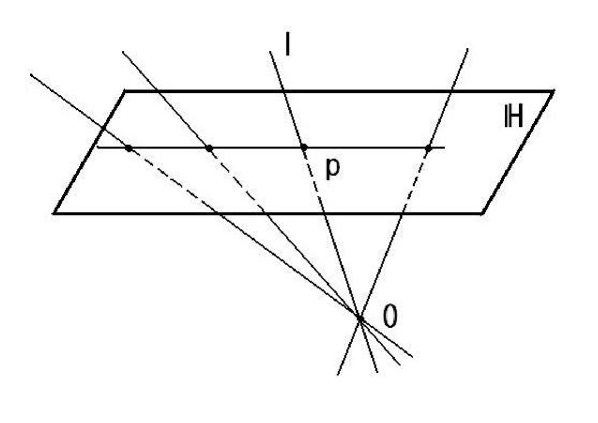
Now, is identified with in a natural manner. We call the homogeneous coordinate of the “point” when passes through , and write by convention. This concept is immediately generalized to , and also to the realm of complex numbers.131131131One can consider the projective planes over quaternions and octonions as well. It is interesting to point out that Desargues’ theorem holds for quaternions, but does not for octonions, and that Pappus’ hexagon theorem does not hold for quaternions. The simplest case is the complex projective line , which coincides with the Riemann sphere, the complex plane plus a point at infinity, introduced by Riemann (fn. 121). A projective transformation in this case is represented as .
Henri Poincaré (1854–1912) observed a conflation of and non-Euclidean geometry in his study of Fuchsian functions (a sort of “periodic” functions of one complex variable). Indeed, the above with satisfying preserves not only , but also . Since is a model of the non-Euclidean plane (fn. 126), is a non-Euclidean congruent transformation.132132132Poincaré, Sur les Fonctions Fuchsiennes, Acta Math., 1 (1882), 1–62. For this reason, is called the Poincaré half plane. The line element was previously obtained by Liouville through transformation of the line element on the pseudosphere (1850). More conspicuously, this idea led up to an entirely new phase of analytic number theory (initiated by Euler and definitively established by Dirichlet) through the notion of automorphic form, a generalization of Fuchsian functions.
Another non-Euclidean model that is cross-fertilized by projective geometry was given by Beltrami in his Saggio and independently by F. Klein (1871). This model, called the Klein model and first constructed in 1859 by A. Cayley in the context of real projective geometry without reference to non-Euclidean geometry (1859), is realized as the open unit disk , in which the “line segments” are chords in . Worthy of mention is that the cross-ratio pops up in the distance between two points. To be exact, the distance between two points and in can be expressed as , where are the points of intersection on the circle with the line connecting (see Remark 17.2 (5)). This distance is the one associated with .
17 Absolute differential calculus
Riemann’s work was evolved further by Elwin Bruno Christoffel (1829–1900) and Rudolf Lipschitz (1832–1903). The significance of Christoffel’s work lies in his introduction of the concept later called covariant differentiation and of the curvature tensor which crystallizes the notion of Riemann’s curvature (1869).133133133Über die Transformation der homogenen Differentialausdrücke zweiten Grades, J. für die Reine und Angew. Math., 70 (1869), 46–-70; Über ein die Transformation homogener Differentialausdrücke zweiten Grades betreffendes Theorem, ibid., 241–245. After a while, Gregorio Ricci-Curbastro (1853–1925) and Tullio Levi-Civita (1873-1941) initiated “absolute differential calculus”134134134Méthodes de calcul différentiel absolu et leurs applications, Math. Ann., 54 (1900), 125–201.—calculus, in line with Christoffel’s work, dealing with “invariant” geometric quantities (called tensor fields). Levi-Civita further brought in parallel transports as a partial generalization of parallel translations.135135135Nozione di parallelismo in una varietàqualunque e consequente specificazione geometrica della curvatura Riemanniana, Rend. Circ. Mat. Palermo, 42 (1917), 73–205. Before long, absolute differential calculus was renamed “tensor calculus” and used effectively by Einstein for his general relativity.136136136Die Feldgleichungen der Gravitation. Sitzungsberichte der Preußischen Akademie der Wissenschaften zu Berlin: 844–847 (November 25, 1915). In this groundbreaking theory, a slight modification of Riemann’s theory is required; namely, the matrix associated with the first fundamental form is a four-by-four symmetric matrix with three positive and one negative eigenvalue. A manifold with such a fundamental form is called a curved space-time, or a Lorentz manifold after Hendrik Anton Lorentz (1853–1928).
We shall now plunge ourselves into tensor calculus. Henthforth the matrix is supposed to be invertible, so that our discussion includes the case of Lorentz manifolds. A tensor field (in the classical sense) is roughly a system of multi-indexed functions depending on the choice of a coordinate system and satisfying a certain transformation rule under coordinate transformations so as to yield a coordinate-free quantity. Tensor fields thus defined fit in with the principle of relativity which Einstein set up to claim that the laws of physics should have the same form in all admissible coordinate systems of reference.
An example is the coefficients of the first fundamental form (called the metric tensor). Here we should note that is a coordinate-free quantity. If we take another coordinate system , we have a different expression . The chain rule for differentiation applied to the coordinate transformation is written as . So substituting this for (15.1), we obtain . Comparing this with , we have the transformation rule .
Another example is a contravariant vector obeying the rule . For instance, for a curve is a contravariant vector because . Hence, a contravariant vector is reckoned as a vector tangent to the manifold.
A general tensor field (of type ) is a system of multi-indexed functions satisfying the transformation formula
Hence is a tensor field of type . For the inverse matrix , we have , so that is a tensor field of type .
The covariant derivative of is a tensor field of type given by
where
| (17.1) |
is what we call the Christoffel symbol.137137137The symbol Christoffel used is . R. Lipschitz (reputable for “Lipschitz continuity”) brought in a simiar symbol in his Untersuchungen in Betreff der ganzen homogenen Functionen von n Differentialen, J. für die Reine und Angew. Math., 70 (1869), 71-102. The terms involving the Christoffel symbols is thought of as making the derivation intrinsic. The curvature tensor is then defined to be a tensor that measures non-commutativity of covariant differentiation; namely, , where
Although being implicit, the curvature tensor turns up in Riemann’s paper submitted to the Académie des Sciences on July 1, 1861 (remained unknown until 1876).138138138Commentatio Mathematica, qua respondere tentatur quaestioni ab , Academia Parisiensi propositae. In the second half of this paper, which was his answer to the prize question on heat distribution posed by the Academy in 1858, he gave a condition in order that is flat, or equivalently that there exists a curvilinear coordinate system such that . His condition can be transliterated into (see [9] for the detail).
We defer the details of how the curvature tensor is linked with Riemann’s sectional curvature (see Sect. 20), and only cite the fact that the Gaussian curvature of a surface is expressed as , so that is a rational function (not depending on ) in and their derivatives up to second order as shown by Gauss with “bare hands” (Disquisitiones generales, Arts. 9-11). More specifically (in the present notation),
Now take this for granted. For an isometry , the composition gives a local parametric representation of such that , , because preserves . Therefore the derivatives of of any order coincide with the corresponding derivatives of , from which Gauss’s Theorema Egregium follows.
Remark 17.1
The following formulas are due to Gauss, K. M. Peterson, G. Mainardi, and D. Codazzi:
| (17.3) | |||
| (17.4) |
In 1867, Bonnet proved the converse (the fundamental theorem of surface theory): if functions and in variables and satisfy (17.3), (17.4), (17), while , then there exists a unique surface (up to motion) in space which admits and as the coefficients of the first and second fundamental forms.
In terms of the Christoffel symbol, the equation of a geodesic is expressed as
| (17.5) |
This expression in a curved space-time—in alliance with imaginary experiments carried out within a closed chamber in interstellar space to confirm the equivalence of gravity and acceleration139139139The freely floating chamber produces a gravity-free state inside, while the accelerated chamber produces a force indistinguishable from gravitation.—is the starting point of Einstein’s theory; that is, we think of (17.5) as an analogue of the Newtonian equation of motion under gravitational potential (i.e., the equation for “free fall”).140140140Grundlage der allgemeinen Relativitätstheorie, Ann. der Physik, 49 (1916), 769–822. Pursuing this analogy, he concluded that the first fundamental form may be loosely regarded as a generalization of the gravitational potential,141141141In his thesis (Part III, §3), Riemann prophetically says, “We must seek the ground of its metric relations outside it, in binding forces which act upon it.” and that the fundamental interaction of gravitation as a result of space-time being curved by matter and energy is manifested by the field equations:
| (17.6) |
where is the Ricci tensor, is the scalar curvature (note that for a surface ), is the cosmological constant,142142142This constant is used to explain the observed acceleration of the expansion of the universe. (In 1929, E. Hubble discovered that the universe is expanding.) is the speed of light in vacuum, and is the stress–energy tensor (an attribute of matter, radiation, and non-gravitational force fields).
The left-hand side of (17.6) as an operator acting on is a non-linear generalization of the d’Alembertian showing up in the description of wave propagation with speed . This observation brought Einstein to the prediction of gravitational waves, which was successfully detected by the Laser Interferometer Gravitational-Wave Observatory (11th February, 2016).
What is remarkable is, as observed by Hilbert (1915), that the vacuum field equations () are the E-L equation associated with the action integral: .
Remark 17.2
(1) D’Alembert showed that solutions of the wave equation are of the form , where and are any functions (1747). On the other hand, Daniel Bernoulli (1700–1782), a son of Johann Bernoulli and a friend of Euler, came up with trigonometric series for the first time, when he tried to solve the wave equation (1747). The two ways to express solutions stirred up controversy on the nature of “arbitrary” functions (Remark 19.1).
(2) The Laplacian named after Laplace appears in the theory of heat conduction by Jean Baptiste Joseph Fourier (1768–1830). While he was Governor of Grenoble (appointed by Napoleon I), he carried out experiments on the propagation of heat along a metal bar, and used the trigonometric series to solve the heat equation that describes the distribution of heat over a period of time (1807 and 1822); see Remark 19.1. An interesting fact is that a special solution is given by the function , which shows up as the normal distribution in mathematical statistics that A. de Moivre, Gauss, and Laplace pioneered.
(3) (17.6) is also regarded as an analogue of Poisson’s equation , where is the gravitational potential associated with a mass density .143143143The density for a mass distribution is defined by the relation . As noticed by Green (1828) and Gauss (1839; Werke V, 196–242), this equation embodies the law of universal gravitation (and hence in the vacuum case). Indeed, is a solution of Poisson’s equation.
A heuristic (and intrepid) way to derive (17.6) in the vacuum case is to take a look at the tendency of free-falling objects to approach or recede from one another, which is described by the “variation vector field” , where is a family of solutions of . Clearly satisfies , where is the linear map defined by . Notice that . In turn, the variation vector field for the geodesic equation (17.5) satisfies the apparently similar equation (called the Jacobi equation), where , and , the covariant derivative of a vector field along the curve (Sect. 20). Since , we may regard the equation (or since is arbitrary) as an analogue of .
(4) The theory of special relativity created by Einstein in 1905 is literally a special case of general relativity, which has radically changed our comprehension of time and space.144144144Zur Elektrodynamik bewegter Körper, Ann. der Physik, 17 (1905), 891–921. Roughly speaking, it is a theory of space-time under absence of gravitation. Einstein assumed that (i) the speed of light m/s) in a vacuum is the same for all observers, regardless of the motion of the light source, and (ii) the physical laws are the same for all non-accelerating observers (this is a special case of the principle of relativity). His setup squares with the theory of electromagnetic waves due to James Clerk Maxwell (1831–1879); see Sect. 22. The special relativity was mathematically formulated by Hermann Minkowski (1864–1909).145145145Minkowski, Raum und Zeit, Physikalische Zeitschrift 10 (1907), 75–88. His model (called the Minkowski space-time) is a 4D affine space with a coordinate system for which the line element is given by . Such a coordinate system (stemming from the invariance of the speed of light) is called an inertial system, which an observer employs to describe events in space-time. If is another inertial system moving in uniform velocity relative to , then the relation between them is given by an inhomogeneous Lorentz transformation:
| (17.7) |
(, , and , ). The matrix satisfies
where is the orthogonal projection of onto the line . Since , the vector is the relative velocity of two systems. Equation (17.7) tells us that the relative speed cannot exceed . Notice that, formally making tend to infinity, we obtain a Galilei transformation compatible with Newtonian mechanics:
With (17.7), one may interpret the Lorentz-FitzGerald contraction of moving objects. Before special relativity came out, Lorentz and G. F. FitzGerald posited the idea of contraction to rescue the existence of aether (or ether) from a paradox caused by the outcome of Michelson-Morley experiment (1887).146146146 Aether, whose existence was discarded by Einstein, had been thought to permit the determination of our absolute motion and also to allow electromagnetic waves to pass through it as elastic waves. Going back into history, ancient thinkers (e.g. Parmenides, Empedocles (ca. 490 BCE–ca. 430 BCE), Plato, Aristotle) assumed that aether (Αἱϑήρ) filled the celestial regions. Descartes insisted that the force acting between two bodies not touching each other is transmitted through it (Traité du monde et de la lumière, 1629–1633). Newton suggested its existence in a paper read to the Royal Society (1675). Riemann assumed that both “gravitational and electrostatic effects” and “optical and magnetic effects” are caused by aether (1853), while Kelvin, holding Newton in reverence, said that he could not be satisfied with Maxwell’s work until a mechanical model of the aether could be constructed (1884).
(5) The linear part of the transformation given in (17.7) with belongs to , where is the matrix group (called the Lorentz group) that preserves the quadratic form . Interestingly, the subgroup of that preserves the sign of the last coordinate comes up as the congruence group for the Klein model (note that the set is identified with , and that the projective transformation associated with a matrix in leaves (and ) invariant and preserves the distance on because of the projective invariance of cross-ratios).
18 Cantor’s transfinite set theory
Mathematical terminology to formulate what Riemann wanted to convey had not yet matured enough in his time. Here is an excerpt from Riemann’s paper referred to above, which indicates how he took pains to impart the idea of manifolds with immatured terms.
If in the case of a notion whose specializations form a continuous manifold, one passes from a certain specialization in a definite way to another, the specializations passed over form a simply extended manifold, whose true character is that in it a continuous progress from a point is possible only in two directions, forwards or backwards. If one now supposes that this manifold in its turn passes over into another entirely different, and again in a definite way, namely so that each point passes over into a definite point of the other, then all the specializations so obtained from a doubly extended manifold. In a similar manner one obtains a triply extended manifold, if one imagines a doubly extended one passing over in a definite way to another entirely different; and it is easy to see how this construction may be continued. If one regards the variable object instead of the determinable notion of it, this construction may be described as a composition of a variability of dimensions out of a variability of dimensions and a variability of one dimension (English translation by Clifford).
Poincaré attempted to give a definition of manifold for his own motivation. In the ground-breaking work Analysis Situs (J. École Polytech, 1 (1895) 1–121), he offered two definitions, both of which rely on “constructive procedures.” The first is to describe a manifold as the zero set of a smooth function , where is an open set of , and the Jacobian of is of maximal rank everywhere. In the second, a manifold is produced by a “patchwork” of a family of open sets of . Although his definitions are considered a precursor to the modern formulation of manifolds, it was not yet satisfactory enough ([33] and [23]). To remove the ambiguity in the early formulation and to study a global aspect of manifolds, it was necessary to establish the notion of topological space, an ultimate concept of generalized space allowing us to talk about “finite and infinite” in an entirely intrinsic manner (thus one can say that topological spaces are “stark naked” models of the universe).
What should be accentuated in this development, is the invention of (transfinite) set theory by Georg Cantor (1845–1918). His Grundlagen einer allgemeinen Mannigfaltigkeitslehre (1883) was originally motivated by the work of Dirichlet and Riemann concerning trigonometric series (Remark 19.1),147147147In Über die Ausdehnung eines Satzes aus der Theorie der trigonometrischen Reihen, Math. Ann., 5 (1872), 123–132, he defined real numbers, using Cauchy sequences of rationals. and made a major paradigmatic shift in the sense that since then mathematicians have accepted publicly “the actual infinity”, as opposed to the traditional attitude towards infinity.148148148Bernhard Bolzano (1781–1848) conceived the notion of set from a philosophical view (Wissenschaftslehre, 1837). To grasp the atmosphere before set theory came in, we shall quote Gauss’s words. In a letter addressed to Schumacher (July 12, 1831), he says, “I protest against the use of infinite magnitude as something completed, which is never permissible in mathematics. Infinity is merely a way of speaking, the true meaning being a limit which certain ratios approach indefinitely close, while others are permitted to increase without restriction” (Werke, VIII, p. 216). What he claimed is not altogether inapposite as far as “differentiation” is concerned, but cannot apply to infinity embodied by set theory.
A set (Mengenlehre) is, as Cantor’s declares, a collection of definite, well-distinguishable objects of our intuition or of our thought to be discerned as a whole.149149149Beiträge zur Begründung der transfiniten Mengenlehre, Math. Ann., 46 (1895), 481-512. This is Cantor’s last major publication. To tell how set theory is linked to the issue of infinity, let us take a look at natural numbers. We usually recognize natural numbers as potential infinity; that is, we identify them by a non-terminating process such as adding 1 to the previous number, while Cantor thinks that one may capture the “set” of all natural numbers as a completed totality (which we shall denote by ). Once the notion of set as the actual infinity is accepted, one can exploit one-to-one correspondences (OTOC) to compare two infinite sets as Archimedes, Bradwardine, and Oresme did (Sect. 2). In this context, infiniteness of a set is characterized by the property that it has a OTOC with a proper subset. This characterization (due to Dedekind) resolves Galileo’s paradox mentioned in Sect. 2, simply by saying that the set of natural numbers is infinite.
The most significant discovery by Cantor is the existence of different sizes of infinite sets; for instance, the real numbers are more numerous than the natural numbers. Thus , the set of real numbers, cannot be captured as potential infinity whatsoever. This was mentioned in a letter150150150Briefwechsel Cantor-Dedekind, eds. E. Noether and J. Cavailles, Paris: Hermann. to Dedekind dated December 7, 1873 and published in 1874. 151151151 His diagonal argument was given in Über eine elementare Frage der Mannigfaltigkeitslehre. Jahresbericht der Deutschen Mathematiker-Vereinigung, 1 (1890–1891), 75–78. Furthermore, he introduced cardinal numbers as a generalization of natural numbers; that is, a cardinal number is defined to be a name assigned to an arbitrary set, where two sets have the same name if and only if there is a OTOC between them.
At any rate, the notion of set per se is so simple that it seem not necessary to take it up expressly. Indeed, “set” is nearly an everyday term with synonyms such as “collection,” “family,” “class,” and “aggregate.” In truth, people before Cantor more or less adapted themselves to “sets” without noticing that the notion cannot be discussed separately from actual infinity.
Greek thinkers were timid with infinity since it often leads to falsity (remember the erroneous argument by Antiphon and Bryson in “squaring the circle”). Cantor, too, struck a snag when he put forward his theory, if not the same snag the Greeks struck. In fact, the simplicity of the notion of set is deceptive. Unless the concept of set is suitably introduced, we run into a contradiction like Russell’s paradox discovered in 1901, which had disquieted, for some time, mathematicians of the day who were favorably disposed towards set theory.152152152His paradox results from admitting that is a set. In fact, if , then by definition, and if , then again by definition.
Surely, Cantor’s innovation was unorthodox and daring at that time; he met with belligerent resistance from a few conservative people. For instance, Poincaré poignantly said that there is no actual infinity since mathematics accepting it has fallen into contradiction (1906), and L. J. J. Wittgenstein bluntly dismissed set theory as “utter nonsense,” and “wrong.”153153153See “Wittgenstein’s Philosophy of Mathematics” in the Stanford Encyclopedia of Philosophy. The frustration and despair caused by the disinterest and cold rejection directed Cantor to a theological explanation of his theory, which, he believed, would open up a whole new landscape in Christian theology (a letter to C. Hermite, dated January 22, 1894 ([18]).
Fortunately, various paradoxes derived from a vague understanding were resolved by axiomatizing set theory,154154154Axiomatic set theory, established by E. Zermelo in 1908 and A. Fraenkel in 1922, is formulated with a formal logic. and most mathematicians responded favorably to his theory. Hilbert, who stands squarely against the outcry of conservative people, exclaims, “No one shall expel us from the Paradise that Cantor has created” (Über das Unendliche, Math. Ann., 95 (1926), 161–190).155155155In the late 1920s, Hilbert preferred to compare the use of actual infinity to the addition of points at infinity in projective geometry.
19 Topological spaces
The swift change caused by set theory delimited the history of mathematics. The old thought that mathematics is the science of quantity, or of space and number, has largely disappeared. From then on, mathematics has been built eventually on set theory, indissolubly combined with the concept of mathematical structure—in short, any set of objects along with certain relations among those objects—which was put forward in a definitive form by Bourbaki in the campaign for modernization of mathematics. An instructive example is whose structure is characterized by Peano’s axioms, the setting that epitomizes the transition from potential infinity to actual infinity (1889):
“The set has an element and an injective map such that (i) , (ii) if is a subset of with and , then .”
Algebraic systems such as groups, rings, and vector spaces are sets with structures as well. Topological spaces are another exemplary, which has, in no small part, evolved out of a long process of understanding the meaning of “limit” and “continuity” of functions.
Remark 19.1
A primitive form of functions is glimpsed in the Almagest, Book 1, Chap. 11. He made a table of chords of a circle (dating back to Hipparchus), which, from a modern view, can be thought of as associating the elements of one set of numbers with the elements of another set. After Oresme (1350), Galileo (1638), and Descartes (1637) adumbrated germinal ideas, the great duo of Johann Bernoulli and Leibniz adopted the word “functio” for “a quantity formed from indeterminate and constant quantities” (1694). A more lucid formulation was given by Euler, who introduced the notation (1734) and defined a function to be an analytic expression composed in any way whatsoever of the variable quantity and numbers or constant quantities” (Introductio; [13]). But, after a while, he altered this definition as “When certain quantities depend on others in such a way that they undergo a change when the latter change, then the first are called functions of the second” ([8]).
Interest in the true nature of functions was renewed when Fourier claimed that an arbitrary function on can be expressed as a trigonometric series
| (19.1) | |||
However, he did not turn his eye to the convergence of the series, let alone the meaning of the equality, the unavoidable issues as pointed out by Cauchy (1820).156156156The bud of the issue is seen in the debate among D’Alembert, Euler, and Daniel Bernoulli about solutions of the wave equation (Remark 17.2 (1)). It was in this context that Cauchy gave a faultless definition of continuous function, using the notion of “limit” for the first time.157157157Euler thought of “” (resp. “”) as “the value for infinitely large (resp. the value for infinitely small”). The modern definition was furnished by Bolzano in his Der binomische Lehrsatz, 1816; however, being of little noticed at the time. Following Cauchy’s idea, Weierstrass popularized the - argument in the 1870’s, which made it possible to discuss diverse aspects of convergence. In the meantime, Dirichlet made Fourier’s work rigorous on a clearer understanding of (dis)continuity. With some prodding from Dirichlet, Riemann made further progress by giving a precise meaning to integrability of function.158158158Riemann, Über die Darstellbarkeit einer Function durch eine trigonometrische Reihe, Abhandlungen der Königlichen Gesellschaft der Wissenschaften zu Göttingen, 13 (1868), 87–132. This was presented in December of 1853 as his Habilitationsschrift at the first stage.
The rigor of calculus whose absence was deplored by Abel was now in place (Remark 4.2 (4)). Analysis that developed on it (and was accompanied with Cantor’s set theory) contributed to the advent of the concept of topological space.
A topology on a set is a family of subsets (called neighborhoods) which makes it possible to express the idea of getting closer and closer to a point and also to introduce the notion of continuous maps as a generalization of continuous functions. In his magnum opus Grundzüge der Mengenlehre (1914), Felix Hausdorff (1869–1942) sets the four axioms in terms of neighborhoods, the last being known as the Hausdorff separation axiom; thus his topological spaces are what we now call Hausdorff spaces, a proper generalization of metric spaces.159159159The earlier results on topology—ascribed to F. Riesz, M. R. Fréchet, and others—fitted naturally into the framework set up by Hausdorff. Currently, there are several ways to define topological spaces; e.g. by the axioms on the closure operation (1922) due to K. Kuratowski, and by the axioms on open sets (1934) due to W. F. Sierpiński. The notion of metric space was first suggested by Fréchet in his dissertation paper (1906).
Now, a manifold with the first fundamental form is a metric space, so we are tempted to discuss finiteness of the universe in the topological framework. Finiteness of a figure in is interpreted by the terms closed and bounded. Thus the issue boils down to the unequivocal question of how we define such terms in an intrinsic manner, without referring to “outside.” The answer is afforded by the notion of compactness (Fréchet, 1906), which expresses “closed and bounded in itself” so to speak, whose origin is the Bolzano-Weierstrass theorem and the Heine-Borel theorem in analysis.
Armed with the impregnable language of finiteness, one may call into question, without assessing relevance to metaphysical or theological meaning, whether our universe is finite. Yet, this overwhelming question is beyond the scope of this essay and belongs entirely to astronomy. The recent observation (by the Planck, the space observatory operated by the European Space Agency) lends support to an “almost” flat model of the universe in the large. However this does not entail its infiniteness since “flatness” does not imply “non-compactness.” In turn, if there are only finitely many particles in the whole universe, then the universe should be finite (here it is assumed that the mass would be uniformly distributed in the large).160160160In the Letter to Herodotus, Epicurus (341 BCE–270 BCE), an adherent of atomism and advocate of “billiard ball universe,” states that the number of atoms is infinite. This seems not to be a foolhardy hypothesis altogether. The cosmological principle in modern cosmology claims that the distribution of matter in the universe is homogeneous and isotropic when viewed on a large enough scale. Einstein says, “I must not fail to mention that a theoretical argument can be adduced in favor of the hypothesis of a finite universe.”161161161Geometry and Experience, an address to the Berlin Academy on January 27th, 1921. Truth be told, however, nobody could definitively pronounce on the issue at the moment. On this point, our intellectual adventure cannot finish without frustration since the issue of finiteness is the most fundamental in cosmology.
20 Towards modern differential geometry
After the notion of topological space took hold, mathematicians got ready to move forward. What had to be done initially was to link the concept of curvilinear coordinate system with topological spaces. An incipient attempt was made by Hilbert, who, using a system of neighborhoods, tried to characterize the plane.162162162Appendix IV (1902) to Grundlagen der Geometrie. Subsequently, Hilbert’s former student Hermann Klaus Hugo Weyl (1885–1955) published Die Idee der Riemannschen Fläche (1913), a classical treatise that lays a solid foundation for complex analysis initiated by Riemann (fn. 121). His perspicuous exposition, though restricted to the 2D case, opened up the modern synoptic view of geometry and analysis on manifolds. Stimulated with this, O. Veblen and his student J. H. C. Whitehead gave the first general definition of manifolds in their book The foundations of differential geometry, 1933. At around the same time, Hassler Whitney (1907–1989) and others clarified the foundational aspects of manifolds during the 1930s. One of significant outcomes is that any smooth manifold (with an additional mild property) can be embedded in a higher-dimensional Euclidean space (1936), thus giving a justification to one of Poincaré’s definitions of manifold (Sect. 18).
Meanwhile, differential geometry of surfaces was expanded by Jean-Gaston Darboux (1842–1917). He published, between 1887 and 1896, four enormous volumes entitled Leçons sur la théorie générale des surfaces et les applications géométriques du calcul infinitésimal, including most of his earlier work and touching on global aspect of surfaces to some extent. Darboux’s spirit was then inherited by Élie Cartan (1869–1951). Most influential is his meticulous study of symmetric space (1926), a class of manifolds with an analogue of point symmetry at each point, including , , , and ; thus unifying various geometries in view of symmetry and also following the Greek tradition in seeking symmetric shapes. Remarkable is that Cartan’s list includes symmetric spaces described in terms of quaternions and octonions. Futhermore Cartan enlarged Klein’s “Erlangen Program” (fn. 43) so as to encompass general geometries.
A decade from 1930 was the period when geometry began to be intensively studied from a global point of view, in concord with a new field launched by Riemann and Poincaré (see Sect. 21). What is more, the fundamental concepts have been made more transparent by means of a coordinate-free setup, which is, in a sense, conform to the principle of relativity in a perfect way.163163163Grassmann was the first to realize the importance of the coordinate-free concepts.
In what follows, just to make our story complete, we shall quickly review, at the cost of some repetition, how some of the ingredients introduced by forerunners are reformulated in modern terms. The first is the definition of smooth manifolds as a terminus ad quem of our journey to “generalized curved spaces.”
Definition (1) A Hausdorff space is said to be a -dimensional topological manifold (or -manifold) if each point of has an open neighborhood homeomorphic to an open set in ; therefore we have an atlas of local charts; that is, a family of curvilinear coordinate systems that covers .
(2) A topological manifold is called smooth if there is an atlas such that every coordinate transformation is smooth (such an atlas is said to be smooth).
Using a smooth atlas, we may discuss “smoothness” of various objects attached to smooth manifolds; say, smooth functions and smooth maps. What comes next to mind is the question whether it is possible to define tangent space as the generalization of tangent planes of a surface. The idea to conceptualize tangent space without reference to a coordinate system and ambient spaces dates back to the work of C. Bourlet who, paying special attention to the product rule, gave an algebraic characterization of differentiation.164164164Sur les opérations en général et les équations différentielles linéaires d’ordre infini, Ann. Ec. Normale, 14 (1897), 133–190.
To explain the idea in depth, we shall first observe that a tangent plane of a surface can be intrinsically defined. Let be the space of vectors tangent to a surface at , and let be the set of smooth functions defined on a neighborhood of . Define the action of on by setting , where is a curve with and . The correspondence has the following properties:
(1) (Linearity) .
(2) (Product rule) .
(3) , .
(4) If for any , then .
We let be the vector space consisting of maps with the properties and . In view of (1), (2), as a map of into belongs to . Hence we obtain a map of into , which turns out to be a linear isomorphism. Identifying with via , we have an intrinsic description of .
The foregoing discussion suggests how to define the tangent spaces of a smooth manifold . Let be the set of smooth functions defined on neighborhoods of , and define to be the vector space consisting of operations satisfying linearity and the product rule.165165165This definition is given in Claude Chevalley’s Theory of Lie Groups (1946). For a curvilinear coordinate system around , partial differentiations () form a basis of . Moreover, the velocity vector for a curve in is defined by putting .
The notion of tangent space allows us to import various concepts in calculus into the theory of manifolds. An example is the differential of a smooth map defined by , which is an intrinsic version of the Jacobian matrix.
A Riemannian manifold is a manifold with a (Riemannian) metric, a smooth family of inner products on (). The relation between the metric and the first fundamental form is given by . A smooth map between Riemannian manifolds is called an isometry if . The differential of an isometry is obviously injective for every . Conversely, for a smooth map of into a Riemannian manifold such that is injective for every , one can equip a metric on (called the induced metric) which makes an isometry. The first fundamental form on a surface is nothing but the metric induced by the inclusion map of into .166166166In 1956, J. F. Nash showed that every Riemannian manifold has an isometric inclusion into some Euclidean space . Furthermore, the metric (15.3) given by Riemann coincides essentially with the standard metric on the sphere that is read in the curvilinear coordinate system derived by the stereographic projection : .
No less important than tangent spaces is the dual space of , which is distinguished from though they are isomorphic as vector spaces. 167167167The distinction between a vector space and its dual was definitively established following the work of S. Banach and his school, though it had been already reflected for a long time by the distinction between covariant and contravariant, and also between cogredient and contragredient, the concepts in group-representation theory. We denote by the dual basis of ; i.e., . The symbol defined in this way justifies the notion of differential (Remark 15.1 (2)). A tensor of type is then a multilinear functional . which is related to a classical tensor by . A tensor field of type is a smooth assignment to each of a tensor of type . A vector field is a tensor field of type . The vector space consisting of all vector fields on is denoted by .
Essential to global analysis are differential forms and their exterior derivative introduced by Poincaré (1886) and Cartan (1899). To give a current definition of differential forms, we denote by the totality of tensors of type satisfying for every permutation of the set . A smooth assignment to each of is called a (differential) -form, all of which constitute a vector space, denoted by . A -form is informally expressed as
where the “wedge product” is supposed to satisfy .168168168The totality of , equipped with the wedge product, constitutes the exterior algebra introduced by Grassmann (Sect. 14). With this notation, the exterior derivation is defined by
Note here that for a smooth function . A significant fact derived from the equality is the identity . Thus we obtain the vector space , which is called the de Rham cohomology group; Remark 21.2 (3).
Differential forms give an incentive to justify the formal expression in multiple integrals, because the basic rules for the wedge product make the appearance of Jacobian determinants automatic: , where is a coordinate transformation. This is in conformity with a change of variables in multiple integrals:169169169This formula was first proposed by Euler for double integrals (1769), then generalized to triple ones by Lagrange (1773). Ostrogradski extended it to general multiple integrals (1836). . Thus we are motivated to make the following definition: “ is said to be orientable if it has a smooth atlas such that the Jacobian determinant of every coordinate transformation is positive” (Poincaré, Analysis Situs, 1895; see Sect. 22). Then, what springs to mind is to define the integral over an orientable -manifold of a -form by setting .
Now, given and a map of an orientable -manifold (possibly with boundary) into , we define the integral of along by , where is defined by setting . This is a generalization of line integrals, with which we may unify Stokes’ formula, Gauss’s divergence theorem, and Green’s theorem, as the generalized Stokes’ formula:
where is a -form on an orientable -manifold with boundary (appropriately oriented), and is the inclusion map.
The notion of vector field is quite old. In his Principes généraux du mouvement des fluides (1755), Euler used it to represent a fluid’s velocity. Related to vector fields is the work Theorie der Transformationsgruppen (1888–1893) by Sophus Lie (1842–1899). Under the influence of Klein’s Erlangen Program, he made the study of infinitesimal group actions, which eventually evolved into the theory of Lie groups. As he observed, giving such an action is equivalent to giving a subspace of satisfying “ ,” where . Here the binary operation (the Lie bracket) satisfies the Jacobi identity . An algebraic system with a similar operation was to be called a Lie algebra.170170170Lie algebra (“infinitesimal group” in Lie’s term) was independently invented by W. Killing in the 1880s with quite a different purpose.
A covariant differentiation acting on tensor fields is an intrinsic generalization of directional differentiation acting on vector-valued functions, which is also designated a connection, a term introduced by H. Weyl (1918). In the case of vector fields, it is a bilinear map satisfying (J.-L. Koszul). Define the functions by the relation . Then
The Levi-Civita connection is a unique connection satisfying
| (20.1) |
The first equality is equivalent to , while the second one tells us that coincides with the Christoffel symbol (17.1).
Let be a smooth curve in . If we write for for brevity, then
With this formula in mind, we define the covariant derivative of a vector field along the curve by setting
If , then is said to be parallel. Since is a system of linear equations of first order, there exists a parallel vector field along satisfying . The parallel transport is then defined by ; thus a connection literally yields a “bridge” between two tangent spaces, originally unrelated to each other. For the Levi-Civita connection, we have in view of (20.1). Therefore preserves the angle between two tangent vectors.
A geodesic is defined to be a curve whose velocity vector is parallel along , i.e., , which, in the case of Levi-Civita connection, turns out to be the E-L equation associated with the functional .
Finally we shall give a modern formulation of curvature. A multilinear map may be defined so as to satisfy
Putting , we obtain the tensor field of type such that . Moreover, taking the subspace of spanned by linearly independent vectors , we obtain the sectional curvature . The Ricci curvature is the quadratic form on , to which the Ricci tensor is linked by .
Remark 20.1
(1) Parallel transports on a surface is related to classical parallelism. Let is a vector field along a curve , and let be the plane tangent to at . Imagine that and are freshly painted and still wet. Roll on in such a way that is a point where the rolled surface at time is tangent to (Cartan rolling; Fig. 13). Then the curve is transferred to a curve in , to a point , and to a vector at . With a little nudge, we can show that is parallel if and only if along is parallel in the classical sense.
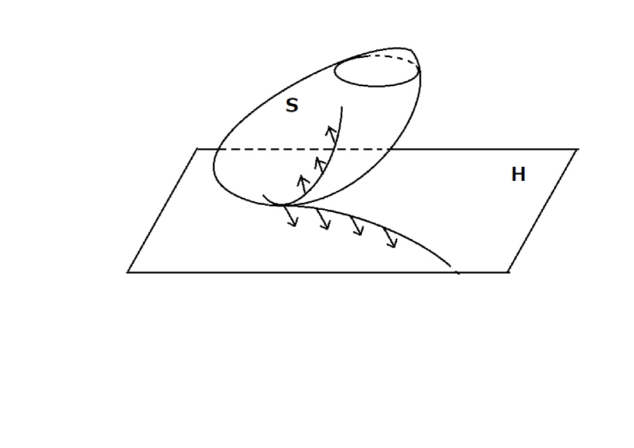
Pushing further this idea, we may construct a one-to-one correspondence between smooth curves in a manifold with and smooth curves in with . Moreover this correpondence extends to the one for continuous curves by means of stochastic integrals, with which we may define Brownian motion on ,171171171“Brownian motion” originally means the random motion of small particles suspended in fluids. It was named for the botanist R. Brown, the first to study such phenomena (1827). In 1905, Einstein made its statistical analysis, and observed that the probabilistic behavior of particles is described by the heat equation (Remark 17.2 (2)). the starting point of “stochastic differential geometry” initiated by K. Ito and P. Malliavin.
(2) The parallel transport around closed loops informs us how a manifold is curved. We shall see this by looking at the parallel transport along the perimeter of a geodesic triangle on a surface . It coincides with the rotation of vectors in through the angle since the parallel transport preserves the angle of two tangent vectors. By virtue of Gauss’s formula (13.1), we find .172172172The idea explained here is generalized in terms of holonomy groups, the concept introduced by É. Cartan (1926).
(3) The idea of connection makes good sense for a vector bundle, a family of vector spaces parameterized by a manifold which locally looks like a direct product, and are used to formulate gauge theory in modern physics that provides a unified framework to describe fundamental forces of nature.
21 Topology of the universe
It cannot be completely denied that the universe may have a complicated structure. Hence it is irresistible to ponder the question “how can we describe the complexity of the universe?” In pursuing this, it will be appropriate to use topological terms as in the case of the question about finiteness.
In passing, the term “topology” used to describe a structure on an abstract set also indicates the branch of geometry which principally put a premium on the properties preserved under homeomorphisms. What, in addition, is important is the concept of homotopy, coined by Dehn and P. Heegaard in 1907, and employed by L. E. J. Brouwer in the current meaning of the word (1911).
A distinct advantage of topology compared with classical geometry is that we can employ lenient operations such as “gluing (pasting)” figures together. For instance, we obtain a sphere by gluing boundaries of two disks (Fig. 14).
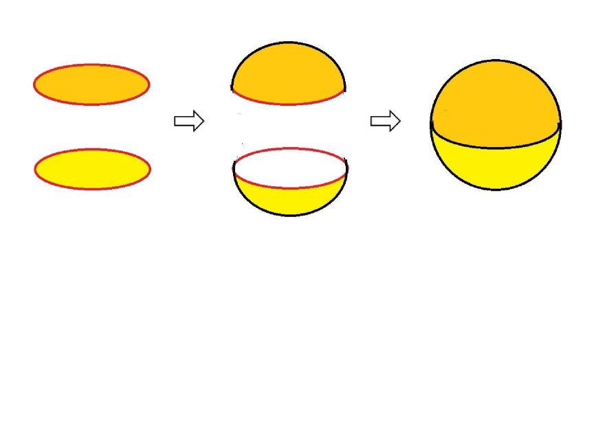
Likewise one can glue boundaries (spheres) of two balls to get the -sphere where one of two balls is the mirror image of another. But this operation cannot be illustrated with drawings, so we shall proceed the other way around; that is, we start with the resulting figure , and put . Clearly and . Furthermore, yields homeomorphisms of onto the ball . This signifies that is obtained by gluing two balls along their boundaries.
This construction of reminds us of an allegorical vision of Christian afterlife in Dante’s poem Divina Commedia. In Canto XXVIII of Paradiso (line 4–9), he “constructs” the empyrean as a mirror image of the Aristotelian universe. Thus, if it were taken at face value (though not a little farfetched), Dante would have obtained as a model of the “universe” ([27]).
Apart from the Dante’s fantastic imagination, the 3-sphere is surely the easiest conceivable model of a (homogeneous and isotropic) finite universe, if not possible to look out it all at once like . Einstein once said that the universe (at any instant of time) can be viewed globally as (see Sect. 18). He wrote, “Now this is the place where the reader’s imagination boggles. ‘Nobody can imagine this thing,’ he cries indignantly. ‘It can be said, but cannot be thought. I can imagine a spherical surface well enough, but nothing analogous to it in three dimensions.’ We must try to surmount this barrier in mind, and the patient reader will see that it is by no means a particularly difficult task” ([6]).
J.-P. Luminet and his colleagues put forward an alternative model of a finite universe with constant positive curvature, which, called the Poincaré homology sphere, is the quotient of by the binary icosahedral group, a finite subgroup of the spin group .173173173J.-P. Luminet, et al., Dodecahedral space topology as an explanation for weak wide-angle temperature correlations in the cosmic microwave background, Nature, 425 (2003), 593–595. Their model—pertinent to the Poincaré conjecture on which we shall comment in due course—explains an apparent periodicity in the cosmic microwave background, electromagnetic radiation left over from an early stage of the universe in Big Bang cosmology.
Remark 21.1
The binary icosahedral group is the preimage of the icosahedral group under the homomorphism of onto (Sect. 7), and is explicitly given as the union of 24 quaternions with 96 quaternions obtained from by an even permutation of all the four coordinates , and with all possible sign combinations ( being the golden ratio).
Solely for the convenience of the reader, let us provide a shorthand historical account of topology. The etymology of “topology” is the German word “Topologie,” coined by J. B. Listing, in his treatise “Vorstudien zur Topologie” (1847) as a synonym for the “geometry of position.” He learned this discipline from Gauss, and launched the study of several geometric figures like screws, knots, and links from the topological perspective. It was Leibniz, if traced back to the provenance of topology, who offered a first rung on the ladder. In a letter to Huygens dated September 8, 1679, Leibniz communicated that he was not satisfied with the algebraic methods in geometry and felt for a different type of calculation leading to a new geometry to be called analysis situs. Leibniz himself did not put his plan into practice, but his intuition was not leading him astray, was embodied by Euler in the solution of the celebrated problem “Seven Bridges of Königsberg” (1736), and also in his polyhedron formula for a convex polyhedron with vertices, edges, and faces, which, stated in a letter to his friend C. Goldbach (November 14, 1750), is recognized as giving a topological characteristic of the sphere (Sect. 13),174174174A copy of Descartes’ work around 1630, which was taken by Leibniz on one of his trips to Paris, reveals that he obtained an expression for the sum of the angles of all faces of a polyhedron, from which Euler’s polyhedron formula can be deduced. and contains some seeds of combinatorial topology pioneered by Poincaré that deals with geometric figures based on their decomposition into combinations of elementary ones.
Gauss took part in the formation of topology, though he opted not to publish any work on topology as usually happened with him. On January 22, 1833 (still in his prime), he noted down a summary of his consideration over the past few months,175175175Nachlass zur Electrodynamik in Gauss Werke, V, translated by Ricca and Nipoti [29]). which was to usher us into the theory of knots and links.
Of the geometria situs, which was foreseen by Leibniz, and into which only a pair of geometers (Euler and Vandermonde were granted a bare glimpse, we know and have, after a century and a half, little more than nothing.
A principal problem at the interface of geometria situs and geometria of magnitudinis will be to count the intertwining of two closed or endless curves.
Let be the coordinates of an undetermined point on the first curve; those of a point on the second and let
| (21.1) |
then this integral taken along both curves is , being the number of intertwinings [called the linking number today]. The value is reciprocal, i.e., it remains the same if the curves are interchanged.
His pretty observation has something to do with electromagnetism. Indeed, (21.1) reminds us of the Biot–Savart law (1820), an equation describing the magnetic field generated by an electric current , which is named after J.-B. Biot and F. Savart. It is stated as
| (21.2) |
where is the magnetic permeability of vacuum (fn. 189).
Another (more pedagogical) example in topology to which Gauss slightly contributed is the notion of winding number. It is defined analytically by
| (21.3) |
where is a closed (not necessarily simple) plane curve that does not pass through . This is an integer because, if we parameterize the curve as with continuous functions and , then, without costing much effort, we see that the integral in (21.3) is transformed into , which, because , represents the total (net) number of times that travels around .
From the analytic expression (21.3) and the fact that an integral-valued continuous function is constant, it follows that, if and are homotopic as maps of the circle into , then . Moreover, does not depend on so far as is in the connected component of containing ; hence one may put .
The homotopy invariance of winding numbers stands us in good stead in proving the fundamental theorem of algebra (cf. Gauss Werke III, 31–56). Given a polynomial , one can take such that , where , so that . On the other hand, if for any , then , so that ; thereby a contradiction, and hence must have a solution.
What deserves a good deal of attention is that the integral (21.3) is neatly expressed as the complex line integral: . Thus as Gauss briefly noticed in the letter to Bessel in 1811 (Sect. 7), the winding number reveals the nature of the complex logarithm (see Remark 8.1).
Winding numbers appeared in the study of “signed areas” by Albrecht Ludwig Friedrich Meister (1724–1788).176176176Generalia de genesifigurarum planarum, et inde pendentibus earum affectionibus, Novi Commentarii Soc. Reg. Scient. Gott., 1 (1769/1770), 144–180. Here, the signed area surrounded by a general closed curve is defined to be . If is simple and counterclockwise, this is the “genuine” area of the domain surrounded by in virtue of Green’s theorem (13.2). For a general and the bounded connected components of , we have
In fact, this is a consequence of the formula holding for any 1-form on , where the boundary is assumed to have counterclockwise orientation. This suggests a formal framework allowing us to write “.” Indeed, this identity can be justified by the notion of “chain” in homology theory (Remark 21.2 (2)).
Moving away from the small treasure trove of Gauss’s “toys”, we shall see how topology evolved thereafter.
The period from the mid-19th century to the early 20th century was the infancy of topology. It coincides with the era when mathematics began to develop autonomously on a rigid base. Prompted by such a state of affairs, geometers created a wealth of novel ideas. One of the marked achievements in this period is the discovery of one-sided surfaces that differ from ordinary surfaces in the way of their disposition in the space. Remember that a smooth surface is two-sided if and only if it admits a global continuous (unit) normal vector field, or equivalently is orientable. (This equivalence is deduced from the fact that, if and are two local parametric representations of a surface with , then , where on The foremost examples of one-side surfaces are the Möbius band and the Klein bottle. The former was discovered by Möbius (1865) and Listing (1862). The latter was constructed by Klein (1882). The projective plane is another example.
The classification of closed surfaces is the problem attacked in the late 19th century. The case of two-sided surfaces was independently treated by Möbius (1863) and M. E. C. Jordan (1866). One-sided closed surfaces were classified by von Dyck (1888). As depicted in Fig. 15, every closed one-sided surface can be constructed from by attaching a finite number of Möbius bands (the leftmost is the projective plane, and the next is the Klein bottle). Thus the “shapes” of 2D models of the finite universe are completely comprehended.
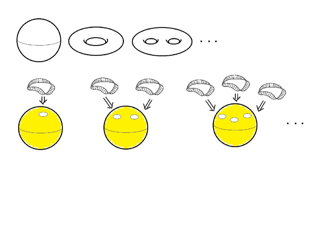
Now, one may ask, “what about the higher-dimensional case?” If restricted to 3- or 4-manifolds, this is a problem concerning a possible structure of our universe, and hence has a much higher profile. More specifically, one may pose the question: Does our universe have a structure like a surface with many holes? Here, the meaning of “hole” is well elucidated in terms of algebraic topology which borrows tools from abstract algebra crystallized in the early 20th century.
Riemann had a clear perception of what we now call the Betti numbers, significant topological invariants related to the Euler characteristic and defined today as the rank of the homology group (see the remark below). His grandiose program—showing again that he was far ahead of the times—was published posthumously as the Fragment aus der Analysis Situs [31]. Later, Enrico Betti (1823–1892), an Italian friend of Riemann, made clearer what Riemann thought.177177177Sopra gli spazi di un numero qualunque di dimensioni, Ann. Mat. Pura Appl., 4 (1871), 140-158. A letter dated October 6, 1863 from Betti to his colleague tells us that he got an accurate conception about the connectivity of spaces through a conversation with Riemann. Finally, their idea came to fruition as homology theory by Poincaré (1899), who also introduced the fundamental group, another algebraic tool and a modern version of “Greek geometric algebra” in a sense because the algebraic system in question are directly constructed from geometric figures.
In the meantime, G. de Rham related homology to differential forms, proving what we now call de Rham’s theorem, one of the earliest outcomes in global analysis (1931). This line—coupled with Chern’s generalization of the Gauss-Bonnet formula (1944) and the theory of harmonic integrals developed by Weyl, W. V. D. Hodge and K. Kodaira—culminated in the Atiyah-Singer theory, one of the most exhilarating adventures of the 20th century. Additionally, the work of M. Gromov on large-scale aspects of manifolds can be considered as far-reaching generalizations of a batch of results on relations between curvature and topology obtained by geometers on and after the 1950s.
The success of the taxonomy of closed surfaces impelled topologists to attack the case of closed 3-manifolds, but the matters turned out to be more complicated than expected. In 1982, W. P. Thurston offered the geometrization conjecture as an initial template, which daringly says that all 3-manifolds admit a certain kind of decomposition involving the eight geometries (one of them is hyperbolic geometry). This spectacular supposition was proved by G. Perelman in 2003. His arguments include the proof of the long-standing Poincaré conjecture which claims, “a simply connected closed 3-manifold is homeomorphic to the 3-sphere.”178178178Poincaré, Cinquième complément à l’analysis situs, Rend. Circ. Mat. Palermo, 18 (1904), 45–110). He claimed, at first, that homology is sufficient to tell if a closed 3-manifold is homeomorphic to (1900), but 4 years later, he found that what we now call the Poincaré homology sphere gives a counterexample. A conspicuity of his proof is that a non-linear evolutional equation involving Ricci curvature is exploited in an ingenious way; thereby displaying a miraculous trinity of differential geometry, topology, and analysis.
The situation gets out of hand when trying to classify closed manifolds with . This is because an arbitrary finitely presented group (a group defined by a finite number of generators, and a finite number of defining relations) can be the fundamental group of a closed 4-manifold, and there is no algorithm to decide whether two finitely presented groups are isomorphic.179179179A. Turing and A. Church rigorously mathematized the concept of algorithm by analyzing the meaning of computation. They independently treated the decision problem challenged by Hilbert in 1928, and showed that a general solution is impossible (1936).
We close this section with an instructive example in differential topology which has been intensively studied in the latter half of the last century.
We shall say that a smooth curve in is regular if for every . Given a closed regular curve , we define the rotation number by setting . In plain language, is the total number of times that a person walking once around the curve turns counterclockwise.180180180As known, at least informally, by Meister (Generalia, 1770), the rotation number is defined for a closed oriented polygonal curve. It is the sum of all (signed) exterior angles divided by (the right of Fig. 16). In the Geometria Speculativa (ca. 1320), Bradwardine (Sect. 2) studied a class of general polygonal curves, which seems to have a relevance with rotation number (Jeff Erickson, Generic and Regular Curves, PDF, 2013). This notion came up in Gauss’s work of experimental nature; he observed, among others (Werke, VIII, 271–281), that, if we denote by the number of self-intersection points of , then we have the sharp inequality: .
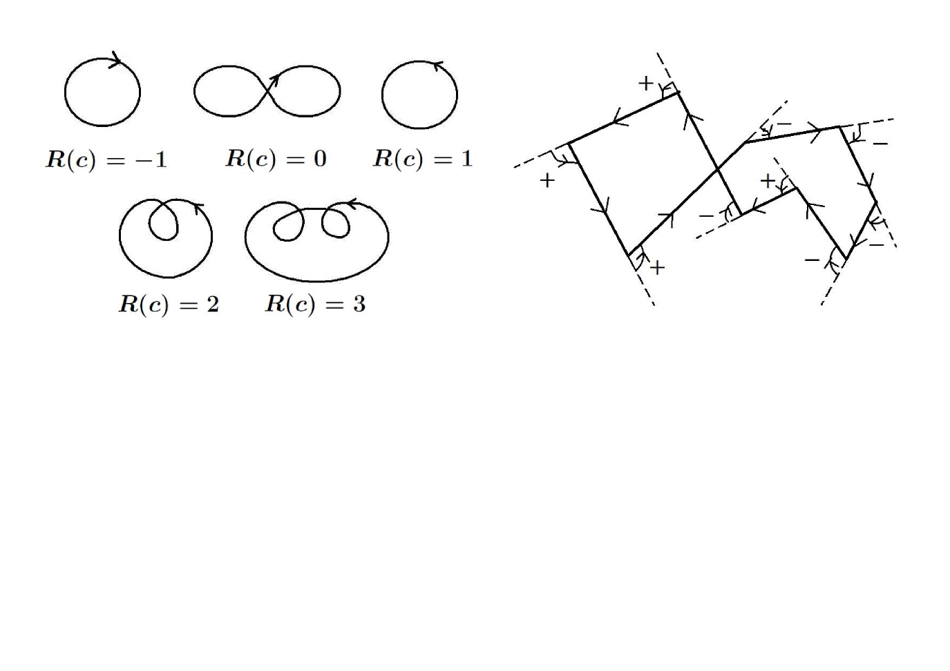
In 1937, H. Whitney proved that a closed regular curve can be deformed to another one through a “smooth” family of closed regular curves (this being the case, two curves are said to be regularly homotopic) if and only if two curves have the same rotation number. In particular, a clockwise oriented circle () is not regularly homotopic to a counterclockwise oriented circle (). This fact is rephrased as “one cannot turn a circle inside-out,” because giving an orientation to a closed regular curve is equivalent to choosing one of two normal unit vector fields along , and the inside and outside of a circle correspond to the inner normal and outer normal vector fields along it, respectively. Of particular note is the unexpected result by S. Smale that one can turn the sphere inside-out, quite by contrast to the case of the circle (1959).
Remark 21.2
(1) The rotation number is linked with the signed curvature (Remark 7.1) via the formula . Indeed,
We thus have a fusion of topology and differential geometry at a very basic level.
(2) In the Analysis situs, Poincaré defined “homology classes” in a somewhat fuzzy way. The group structure on homology classes, which he did not explicitly indicate, was studied by E. Noether and others in the period 1925–28. Later on, S. Eilenberg developed the singular homology theory that allows to define the homology group for a general topological space (1944).
A central role in homology theory is played by a chain complex, a series of homomorphisms satisfying , where, in the singular case, is the free abelian group generated by “singular -simplices” (continuous maps from the -simplex into a topological space ). The -simplex here is a generalization of a segment (), a triangle (), and a tetrahedron (). The homomorphism brings to the sum of the singular -simplices represented by the restriction of to the faces of the -simplex, with an alternating sign to take orientation into account. The factor group is what we call the -th homology group of . The -th Betti number is the rank of (if finite). When for , the Euler characteristic of is defined to be , which, for a surface, agrees with the definition relying on a triangulation (Sect. 13).
(3) For a -form on a convex domain satisfying , there is a -form with ; that is, . This (the Poincaré lemma),181181181Poincaré, Les Méthodes nouvelles da la Mécanique céleste, vol. 3, Gauthier-Villars, Paris, 1899, pp.9–15. This fact, which, in the case of 1-forms, dates back to Euler (1724/1725) and Clairaut, is essentially ascribed to Vito Volterra (1860–1940). in tandem with the generalized Stokes’ formula, is crucial in the proof of de Rham’s theorem asserting that for a closed manifold .
(4) Define the -form on a closed even-dimensional orientable manifold by
Then Chern’s generalization of the Gauss-Bonnet formula is expressed as
(5) Hodge’s theorem says that the space of harmonic forms is isomorphic to , where is the adjoint of (with respect to natural inner products on ). Using this fact, we obtain
| (21.4) |
where , an operator from the space of even forms to the space of odd forms. A special feature of is that it is elliptic; i.e., its principal symbol is invertible.182182182A differential operator of order on (acting on vector-bundle valued functions) is locally expressed as , where denotes a -tuple of non-negative integers, , , and are matrix-valued functions. The principal symbol of is defined to be ().
The left-hand side of (21.4) is called the analytic index of . The Atiyah-Singer theorem asserts that the analytic index () of an elliptic operator equals the topological index defined in terms of topological data, and that there is a -form involving both curvature tensor and principal symbol of such that .
22 Right and left in the universe
An intriguing question about our universe is whether it has “one side” or “two sides.” In discussing sideness, it seems necessary, if looking back to the case of surfaces (Sect. 21), to assume the existence of “outer side” of the universe. The fact is that it is genuinely intrinsic in character as in the case of finiteness. Why is it so? This time, we bring in the idea of “right and left,” the terms used not only in everyday life, but also in mathematics, which are usually designated by the human hands. No less obvious perhaps to our eyes, but no less essential, is the recognition that the human hands are represented by frames (ordered basis), the notion obtained by whittling away the extraneous details of hands; see Fig. 17 illustrating the right-handed frame .183183183The fact that there are just two kinds of frames in is equivalent to that the general linear group has two connected components.
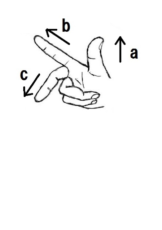
To clarify the nature of right and left, we shall refer to the notorious mirror paradox that is best stated as a question: Why do flat mirrors reverse left and right, but not top and bottom? Prima facie, this sounds puzzling, but the mirror paradox is simply a paradox of “a red herring” or a word play to confuse or startle people by making them believe that the wording “left and right” is the same sort of “top and bottom.” Indeed, the latter is not described by a frame, but by a single vector; say, the vector represented by the directed segment joining bottom and top.184184184Shin-itiro Tomonaga argues that this paradox cannot be resolved by neither geometric optics nor mathematics (1963), while Martin Gardner says that the mirror does not reverse right and left, but does reverse front and back ([10]).
Now, the claim “the universe has two sides” is rephrased as “the right-handed frame and the left-handed frame are distinct wherever they are” in the sense that these two frames cannot be superposed no matter how one is moved to another in the universe. Otherwise expressed, if the universe has “only one side,” then the distinction between the right-handed frame and the left-handed frame does not make sense; namely there is only one kind of frame. What is more, as in the case of surfaces, two-sidedness and orientability of the universe are equivalent when we regard the universe as a smooth manifold. Thus the distinguishability between right and left depends on the global intrinsic structure of the universe.
Even if our universe is Euclidean, there remains a subtle problem on “right and left” that dates back to the dispute between Newton and Leibniz and have fascinated philosophers and cosmologists since then ([12]). Newton insisted that there is a ‘left’ and ‘right’ in the universe, while Leibniz opposed this view and argued that left and right are in no way different from each other.185185185Leibniz’s critique of Newton is unfolded in his third letter to S. Clarke (fn. 54). Puzzled by enantiomorphs for decades, Kant mused about this issue in connection with Leibniz’s claim that all spatial facts should be reduced to facts about relative distances between material bodies (Prolegomena, 1738). He surmised in his prolix discussion that the difference between similar but not congruent things cannot be made intelligible by understanding about any concept, and are known only through sensuous intuition. He even set up an extreme thought-experiment to adduce conclusive evidence of his assertion.186186186Von dem ersten Grunde des Unterschieds der Gegenden im Raume, 1768. In it, he considers a marble hand broken off a statue that is supposed to be the only object in the universe, and asks whether it makes sense to say that it is still either a right hand or a left. According to him, this suggests, after all, that space is not independent of the mind that perceives it.
The purport of what Newton, Leibniz, and Kant thought up is clarified if we replace Kant’s claim by the statement, “one cannot furnish any mathematical characterization of right-handedness of a frame.” This might perplex the reader because, in several places of this essay, we used vector product, whose (casual) definition relies on the right-handed frame; thus seemingly incomplete as a mathematical concept. As a matter of fact, we may select any frame as a reference frame; if we choose another kind of frame, then the resulting vector has the opposite direction, and there is no trouble caused at all.
How about the issue of right and left in physics? Ernst Mach (1838–1916)187187187Mach is best-known for the sensation-based theory of reality. In Die Mechanik in ihre Entwicklung historisch-kritisch dargestellt (1883), he criticized Newton’s conclusion on absolute motion based on the bucket experiment (fn. 52), saying that centrifugal force may act on water in the stationary bucket if the universe rotates. According to him, the inertia and acceleration of a body are determined by all of the matter of the universe. This view was called the Mach principle by Einstein (1918). cogently argued that only asymmetric laws can distinguish left and right (1886). Here, a law is said to be asymmetric (or to violate parity) if it is not invariant under transformations interchanging left and right (specifically, under the parity transformation ). In this connection, the neophyte of physics might recollect Fleming’s left-hand rule about the direction of force acting on a current-flowing wire under an external magnetic field (Fig. 18). As the name suggests, the rule is described by using human hands, and hence seem to imply that the electromagnetic phenomenon is asymmetric. But that is not actually the case because of the nature of magnetic fields. In order to put it clearly, let us recall the Lorentz force experienced by a particle of charge moving with velocity in the presence of an electric field and a magnetic field . Here is not an ordinary (polar) vector, but an axial vector gaining an additional sign flip under a reflection.188188188The distinction between “polar” and “axial” vectors was made by W. Voigt in 1896. Note that and .
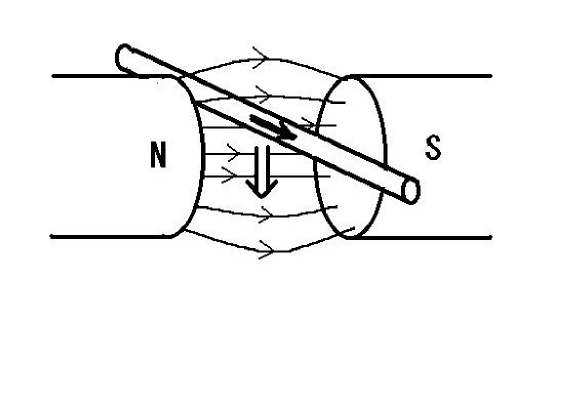
The nature of magnetic fields is more well explained by identifying with the differential 2-form since is “handedness-invariant.” This identification is not altogether artificial, though, at first sight, differential forms might look an elaborate mathematical fabrication, having nothing to do with the real world. To convince ourselves of this, let us employ differential forms to express Maxwell’s equations.
The original form of Maxwell’s equations in a vacuum is:
| (22.1) |
where stands for the dielectric constant of a vacuum,189189189, . Strictly speaking, these equations are Heaviside’s version (1888/1889). Maxwell’s original equations (consisting of 20 equations in 20 variables) are quite complicated. It follows from (22.1) that both and satisfiy the wave equation under the absence of and . Hence electromagnetic waves propagate at the speed , which coincides with the speed of light. Maxwell thus predicted that light is an electromagnetic wave (1865). This was confirmed experimentally by H. Hertz in 1887. and (resp. ) is the density of electric charge (resp. the electric current density). Writing and lumping together the magnetic field and the electric field, define a 2-form by setting . Writing likewise, we put . Then (22.1) are rewritten as , which is manifestly invariant under Lorentz transformations. Here is the adjoint of the exterior derivation with respect to the Minkowski metric; specifically,
for .
It was unthinkable that anyone should question the validity of symmetry under a mirror reflection until a genuine asymmetric law was predicted by T.-D. Lee and C.-N. Yang in 1956 as the parity violation of the weak interaction (a force that governs all matter in the universe). Right after their announcement, the mind-boggling prediction was confirmed by C.-S. Wu and her collaborators through an experiment monitoring the beta decay of cobalt-60 atoms. Expressed in words, this implies that the nature at a very fundamental level can tell the characteristic difference between left- and right-handed (see [10]).
In addition to the weak interaction, there are the three other fundamental interactions in nature; say, the electromagnetic force, the strong interaction, and gravitation. The strong interaction is, loosely put, the mechanism responsible for the strong nuclear force and is known to be “P-symmetric”, i.e., invariant under the parity transformation like the electromagnetic force. In this connection, a few more words about symmetry in quantum physics will not be out of place; besides the P-symmetry, we have the “C-symmetry” under the charge conjugation that reverses the electric charge and all the internal quantum numbers, and the “T-symmetry” under the time reversal replacing by . Each of these symmetries can be violated individually. Theoretically, however, there exists no physical phenomenon that violates the “CPT-symmetry,” the combination of all three symmetries. This fact is called the “CPT theorem.”
23 Conclusion
In retrospect, the theorem of angle-sum and the Pythagorean Theorem in classical antiquity were the fresh impetus in the far-reaching feats by Gauss and Riemann. The triangle inequality as well was a fundamental source of the theory of topological spaces, with which we can get a better understanding of intrinsicness of curved spaces. Moreover, the effort to refine the ancient approach to “infinitesimals” came to fruition as calculus by Newton and Leibniz, which, combined with the idea of coordinate system (no little indebted to Descartes’ method), provided us with a powerful tool to investigate our space. What we ought to remember in particular is Cantor’s set theory that not only encompasses all the necessary stuff for mathematizing cosmology, but also spurred us on to give a probing interpretation to infinity whose nature had been a perennial controversial issue passed from antiquity.
Sullivan [36] says felicitously in a general context, “A history of mathematics is largely a history of discoveries which no longer exist as separate items, but are merged into some more modern generalization, these discoveries have not been forgotten or made valueless. They are not dead, but transmuted.”
References
- [1] L. M. Blumenthal, A Modern View of Geometry, Dover, 1980.
- [2] R. Bonola, Non-Euclidean Geometry: A Critical and Historical Study of its Development, Dover, 2010.
- [3] M. Bossi and S. Poggi, ed. Romanticism in Science: Science in Europe, 1790–1840, Springer; 1993 edition.
- [4] H. S. M. Coxeter, Gauss as a geometer, Historia Mathematica, 4 (1977), 279–396.
- [5] Descartes, The Geometry of Rene Descartes with a facsimile of the first edition, translated by D. E. Smith and M. L. Latham, Dover, 1954.
- [6] A. Einstein, Ideas and Opinions, Broadway Books, 1995.
- [7] Euclid, The Thirteen Books of Euclid’s Elements, translated by T. Heath, Dover, 1956 (1908).
- [8] L. Euler, Foundations of Differential Calculus, Springer, 2000.
- [9] R. Farwell and C. Knee, The missing link: Riemann’s “Commentatio,” differential geometry and tensor analysis, Historia Math. 17 (1990), 223–255.
- [10] M. Gardner, The New Ambidextrous Universe: Symmetry and Asymmetry from Mirror Reflections to Superstrings, Third Revised Edition, Dover, 2005.
- [11] L. Giaccardi, Scientific research and teaching problems in Beltrami’s letters to Hoüel, in “Using History to Teach Mathematics”, edited by V. J. Katz, The Mathematical Association of America, (2000), 213–223.
- [12] C. G. Gross and M. H. Bornstein, Left and right in science and art, Leonard Vol. II (1978), 29–38.
- [13] H. N. Janke, Algebraic Analysis in the 18th Century, in “A History of Analysis” edited by Janke, London Math. Soc., (2003), 105–136.
- [14] V. J. Katz, A History of Mathematics: An Introduction, Addison-Wesley, 2009.
- [15] H. Koch, Introduction to Classical Mathematics I: From the quadratic reciprocity law to the uniformization theorem, Springer, 1991.
- [16] A. Koyré, From the Closed World to the Infinite Universe, The John Hopkins Press, 1957.
- [17] N. I. Lobachevsky, Pangeometry, edited and translated by A. Papadopoulos, European Math. Soc., 2010.
- [18] H. Meschkowski, Aus den Briefbüchern Georg Cantors, Arch. Hist. Exact Sci., 2 (1965), 503–519.
- [19] M. Monastyrsky, Riemann, Topology and Physics, Boston-Basel, 1987.
- [20] S. Negrepontis, Plato on geometry and the geometers, preprint, 2017.
- [21] R. Netz, K. Saito, and N. Tchernettska, A new reading of Method Proposition 14, preliminary evidence from the Archimedes Palimpsest (Part 1 and Part 2), SCIAMVS, 2, (2001), 109–129.
- [22] O. Neugebauer, Zur geometrischen Algebra (Studien zur Geschichte der ntiken Algebra III), Quellen und Studien zur Geschichte der Mathematik, Astronomie und Physik, Abteilung, B. Bd. III (1936), 245–259.
- [23] K. Ohshika, The origin of the notion of manifold: from Riemann’s Habilitationsvortrag onward, in “From Riemann to Differetial Geometry and Relativity” (ed. L. Ji, A. Papadopoulos, S. Yamada), Springer, 2017, 295–309.
- [24] A. Papadopoulos, On Lobachevsky’s trigonometric formulae, Gaṇita Bhārātī (Bull. Indian Soc. Hist. Math.), 34 (2012) , No.1-2, 203–224.
- [25] A. Papadopoulos, On the works of Euler and his followers on spherical geometry, Gaṇita Bhārātī (Bull. Indian Soc. Hist. Math.), 36 (2014) No. 1-2, 237–292.
- [26] A. Papadopoulos and G. Théret, La théorie des lignes parallèles de Johann Heinrich Lambert, Sciences dans l’histoire, 2014.
- [27] M. Peterson, Dante and the 3-sphere, Amer. J. Phys., 47 (1979), 1031.
- [28] R. Rashed and A. Papadopoulos, Menelaus’ ›Spherics‹: Early Translation and al-Mhnī/ al-Harawī’s Version, Walter de Gruyter 2017.
- [29] R. L. Ricca and B. Nipoti, Gauss’ linking number revisited, J. of Knot Theory and Its Ramifications, 20 (2011), 1325–1343.
- [30] J. P. Richter, The Literary Works of Leonardo da Vinci, 1979.
- [31] B. Riemann, Gesammelte Mathematische Werke und Wissenschaftlicher Nachlass, edited with the support of R. Dedekind and H. Weber, Leipzig: Teubner (1876); 3rd ed. by R. Narasimhan, Springer (1990).
- [32] Saccheri, Euclid Vindicated from Every Blemish, edited and annotated by Vincenzo De Risi, translated by G. B. Halsted and L. Allegri, Birkhäser, 2014.
- [33] E. Scholz, The concept of manifold, 1850–1950, in History of Topology, edited by I. M. James, North-Holland, 1999, 25–64.
- [34] M. Spivak, A Comprehensive Introduction to Differential Geometry, Volume 2, Publish or Perish, 1970.
- [35] J. Stillwell, Sources of Hyperbolic Geometry, Amer. Math. Soc., 1996.
- [36] J. W. N. Sullivan, The History of Mathematics in Europe in Europe from the Fall of Greek Science to the Rise of the conception of Mathematical Rigour, Oxford University Press, 1924.
- [37] T. Sunada, The Story of Area and Volume from Everyday Notions to Mathematical Concepts, Chap. 2 in A Mathematical Gift, III: The Interplay Between Topology, Functions, Geometry, and Algebra, translated by Eiko Nakayama Tyler, Amer. Math. Soc., 2005.
- [38] T. Sunada, Topological Crystallography —With a View Towards Discrete Geometric Analysis—, Springer, 2013.