From individual-based epidemic models to McKendrick-von Foerster PDEs: A guide to modeling and inferring COVID-19 dynamics
Abstract
We present a unifying, tractable approach for studying the spread of viruses causing complex diseases requiring to be modeled using a large number of types (e.g., infective stage, clinical state, risk factor class). We show that recording each infected individual’s infection age, i.e., the time elapsed since infection, has three benefits.
First, regardless of the number of types, the age distribution of the population can be described by means of a first-order, one-dimensional partial differential equation (PDE) known as the McKendrick-von Foerster equation. The frequency of type is simply obtained by integrating the probability of being in state at a given age against the age distribution. This representation induces a simple methodology based on the additional assumption of Poisson sampling to infer and forecast the epidemic. We illustrate this technique using French data from the COVID-19 epidemic.
Second, our approach generalizes and simplifies standard compartmental models using high-dimensional systems of ordinary differential equations (ODEs) to account for disease complexity. We show that such models can always be rewritten in our framework, thus, providing a low-dimensional yet equivalent representation of these complex models.
Third, beyond the simplicity of the approach, we show that our population model naturally appears as a universal scaling limit of a large class of fully stochastic individual-based epidemic models, where the initial condition of the PDE emerges as the limiting age structure of an exponentially growing population starting from a single individual.
1 Introduction
1.1 Challenges posed by complex diseases such as COVID-19
The transmission of pathogens between species is a global concern [38, 11]. As such zoonotic episodes are expected to become increasingly common in humans, it is critical to develop analytic tools that can quickly transform epidemiological observations into informed public policy in order to mitigate and control epidemics.
A novel coronavirus, SARS-CoV-2, has recently crossed the species barrier into humans and, within months, has rapidly spread to all corners of our planet [60]. The sheer scale of this pandemic has overburdened our medical infrastructure, caused fatalities estimated well into millions, and shut down entire economies. Remarkably, the rapid spread of COVID-19 and its consequences can be attributed to the unique life cycle of a 30,000 base pair single-stranded virus. SARS-CoV-2 is an airborne pathogen transmitted by both symptomatic and asymptomatic carriers in close proximity to non-infected individuals. Milder COVID-19 symptoms include a dry cough, fever, and/or shortness of breath while more serious cases include respiratory failure and possible death. With millions of infections and hundreds of thousands of documented deaths and recoveries, the COVID-19 pandemic is providing a wealth of independent estimates of important clinical characteristics that can help predict health outcomes specific for a country or region.
It quickly became understood that accurate descriptions of the life cycle of this disease needed to distinguish between several stages of the disease, referred to as compartments, depending on whether an infected individual is infectious or not, symptomatic or not, hospitalized, etc. However it remains unclear to what extent making precise predictions of the dynamics of such a complex disease requires to have a precise knowledge of clinical features such as incubation period, generation time, and duration times between infection, symptom establishment, hospitalization, recovery and death, to know how these durations correlate and what are the exact probabilities of transition between stages.
In this work, we consider a fully stochastic, generic epidemiological model with an arbitrary number of compartments, that encompasses life cycles of most complex diseases and that of COVID-19 in particular. We show how structuring the infected population by its infection age, i.e., time elapsed since infection, allows us to decouple dependencies between stages and to time. More specifically, when the population size is large enough, the joint evolution of all compartment sizes can be described by means of a linear, first-order partial differential equation (PDE) known as the McKendrick-von Foerster equation describing the number of infecteds of (infection) age at time . The boundary condition at age 0 is driven by the infection rate from infecteds of age , averaged over all possible courses of infection, and the number of individuals of age in compartment at time is obtained by thinning by a factor which is the probability of being in compartment conditional on having age , averaged over all possible courses of infection.
In the case of COVID-19, we display a simple procedure to infer these parameters, some from the biological literature and most from time series of numbers of severe cases, hospitalized cases, discharged patients and deaths that can be applied easily to any regional or national dataset. We also allow for time inhomogeneity in the infection rate to account for temporary mitigation measures such as lockdowns or social distancing. We apply this procedure to French COVID-19 data from March to May 2020 and estimate various parameters of interest including the reproduction number in different phases of the epidemic (before, during, and after lockdown) and biological parameter values that we compare to empirical estimates.
1.2 Decorated age-structured epidemic models
The large population size limit of our stochastic model is a PDE “decorated” with compartments. This point of view extends the usual sets of ODEs used in epidemiology, and allows us to represent in the same framework a large class of deterministic epidemic models. Before describing the stochastic model underlying such decorated PDEs, let us illustrate this notion by recalling the well-known derivation of the classic SIR set of ODEs from an age-structured model.
Consider the solution to the following partial differential equation:
| (1) | ||||
where , and fulfill
Equation (1) was first proposed to describe the dynamics of an epidemic where infected individuals are structured by their age of infection, and is known as the Kermack-McKendrick model [36]. Note that in the original work of [36] the model is formulated as the solution to a convolution equation rather than as a PDE, but that the two formulations are equivalent, see Section 2.2. In this context, the age of an individual refers to the time elapsed since its infection, and not to its actual age. Then, is the density at time of all individuals with age (of infection) , and the density of individuals still susceptible to the disease. The differential term describes the aging process: the age of an individual increases linearly with time at rate one. The interpretation of the age boundary condition of (1) is that individuals with age infect susceptible individuals at a rate that only depends on their age.
Remark 1.
It is important to note that counts all individuals that have been infected at time , and not only infective individuals with age . Thus, Eq. (1) lacks the usual recovery term. Moreover, is not the average rate at which infective individuals with age yield infections, but the average infection rate of any individual with age . (The former is obtained from the latter by discounting all individuals with age that are not infectious anymore.)
In order to recover the SIR model, suppose that is given by
for some . Further define
Then a simple calculation shows that solves the following well-known system of ODEs:
| (2) | ||||
The previous expressions have an interesting probabilistic interpretation. Consider a Markov process with two states and . Suppose that it starts from and jumps to at rate . The process can be interpreted as describing the sequence of states (infective then recovered) visited by a typical individual in the microscopic model underlying (2). Then, clearly
so that
| (3) |
Furthermore, suppose that a typical infected individual yields new infections at constant rate while it is in state . Then, the mean number of new infections occurring in the time interval is
The picture that emerges from this simple calculation is that, instead of keeping track of the number of individuals in each compartment, one can consider the age structure of the population, given by Eq. (1). The dynamics of the age structure is uniquely prescribed by the average number of infections that an individual yields at age . The individual counts in each compartment can then be recovered by integrating against the age structure the one-dimensional marginals of a process that describes the sequence of compartments visited by a typical individual in the population. We say that the PDE is “decorated” with compartments, as the process is used to recover the counts in the compartments, and only influences the dynamics of the infection which is described by the sole Eq. (1) through the average infection rate .
This viewpoint has several advantages compared to the usual ODE setting of (2). First, we can make sense of (3) for any process . If this process is not Markovian, the number of individuals in each compartment no longer solves a system of ODEs similar to (2). Hence, this approach allows to go beyond the usual ODE framework. This generalization is of great modeling interest since a hypothesis underlying sets of ODEs is that the sojourn times in each compartment and the time between successive infections are exponentially distributed. In particular they cannot account for sojourn time distributions that are peaked around a value, which have been reported for instance for COVID-19 [41, 58].
Second, regardless of the number of compartments, the age structure of the population is described by the same one-dimensional PDE. This is particularly valuable when models have a large number of compartments, as in the context of COVID-19 [50, 19, 12, 17], as it avoids the use of high-dimensional systems of ODEs that are cumbersome to study mathematically. However, this requires to work with the PDE (1) rather than with ODEs, resulting in a mild computational cost.
Third, Eq. (1) only involves the mean number of infections induced by individuals at age averaged over all compartments. In particular, it is unnecessary to assess to which compartments individuals belong when they yield new infections. This is in contrast with the usual ODE framework, where for each compartment an infection rate needs to be prescribed. As we will see, relates to well-known epidemiological quantities that can be assessed directly from the data.
The main contribution of our work is to show that such decorated age-structured models arise naturally as the law of large numbers limit of a wide class of general stochastic epidemic models that we now introduce.
1.3 Generic stochastic model assumptions
We consider a population model in which individuals are either susceptible, if they have not yet met the disease, or infected. Our definition of infected is broader than usual: an individual is infected if it has been infected in the past. In particular, individuals that have recovered or died from the disease are still infected, even if they are not infective anymore. At any point in time, an infected individual is in one of several states, that will also be referred to as compartments, types, classes, or stages. The set of all such states is denoted by and is assumed to be finite. Depending on the disease complexity, the number of stages can vary. In the SARS-CoV-2 example, typical stages are asymptomatic, mild case, severe case, hospitalized, intensive care unit, recovered, and dead (see Figure 5).
We assume that upon infection a susceptible individual immediately changes state and never becomes susceptible anymore (ruling out multiple infections, in particular), and that it will eventually end in one of two states: recovered or dead. The sequence of states visited by an individual is then encoded by a stochastic process valued in , where the random variable is the state of at age of infection . We call the life-cycle process.
Each individual is further endowed with a random point process on , called the infection point process. Each atom of gives the age at which makes an infectious contact with another individual in the population, and we assume that all atoms are distinct so that secondary infections cannot occur simultaneously. (By an infectious contact, we mean a contact that would lead to a new infection if the target individual is susceptible to the disease. The pair characterizes the course of the infection of individual . We assume that these pairs, for all individuals , are i.i.d. copies of the same pair that describes the infection of a typical individual in the population.
In order to make the mathematical treatment of the model easier, we make the simplifying assumption that the number of susceptible individuals is large compared to the number of infected individuals, so that each infectious contact leads to a new infection. (We neglect the saturation in the number of infections due to the finiteness of the population.) The epidemic is then described by a branching process known as a Crump-Mode-Jagers process [31, 54]: an individual infected at time will produce new secondary infections at times , where are the atoms of , that is ,
(This branching hypothesis is relaxed in a recent work by some of the authors [18].)
Lastly, we superimpose time heterogeneity to this process by means of a contact rate valued in thinning the infection process. More precisely, if is a potential time of infection for individual , we ignore the infection with probability . This contact rate can model the effect of vaccination, or density-dependence (i.e., relaxing the branching assumption due to an excess of removed or of deceased individuals), or of governmental mitigation measures (i.e., social distancing, lockdown).
The infection process is more formally constructed in Section 2.1.
Remark 2.
As already discussed in the previous section, in the SIR example , and is a Markov process started from that jumps to at rate . Moreover, the infection point process is given by
where is a homogeneous Poisson point process on with intensity .
Remark 3.
We emphasize that the pairs are assumed to be independent, but not the variables and . In the simple SIR example they are not independent since there can be no atoms of after the recovery time. In the same spirit, one could assume that the infection potential of a given individual is reduced once in the hospital and that individuals with many atoms in their infection process (high infectiosity) are identified and isolated.
1.4 Statement of the main results
The stochastic epidemic models we consider here are fairly general and can exhibit quite complex dependencies (i) between states and time, due to the lack of any Markov-type assumption, (ii) between states, due to possibly hidden structuring variables impacting the life cycle, (iii) between state and infection rate, and (iv) between past and future infection events. The main result of this work is that despite this apparent complexity, most of this complexity vanishes when the size of the population is large. More specifically, we show that in the limit of large populations (obtained by starting from a large initial population or as a consequence of natural exponential growth), the population of infected individuals structured by age (of the infection) can be described by means of a one-dimensional PDE, and that the counts in each compartment are recovered by decorating this PDE with the life-cycle process. The limiting expression only depends on:
-
1.
The average infection rate
formally defined as the intensity measure of . We make the simplifying assumption that has a density w.r.t. the Lebesgue measure and, with a slight abuse of notation, we still denote it by .
-
2.
The one-dimensional marginals of the life-cycle process
We prove two main theorems that are two laws of large numbers for the age and compartment structure in the population: one started from a large number of individuals, and the other from a single individual.
Large initial population.
Let us start the population with a large number of infected individuals at time , with i.i.d. initial infection ages with law . (See Section 2.1 for a formal definition of the initial age.) Define the empirical measure of ages and compartments at time as
| (4) |
where denotes the infection time of , and the sum is taken over all individuals infected before time . (This includes the initial individuals infected before time .) The measure is a random point measure that encodes the ages and compartments of all individuals that have been infected before time .
Let us also introduce , the number of individuals in compartment at time , defined as
Theorem 1 ( individuals).
Start the population with individuals with i.i.d. initial ages distributed according to . Then, for any , the following convergence holds in the weak topology
where is the solution to
| (5) | ||||
As a consequence, for any ,
| (6) |
The limiting age structure of the population is thus described by Eq. (5), which is a linear version of Eq. (1), known as the McKendrick-von Foerster equation. Note that it also has an additional term accounting for the reduced contact rate, resulting in a time heterogeneity. As in Section 1.2, the number of individuals in each compartment is recovered by decorating the PDE with the one-dimensional marginals of the life-cycle process.
After lockdown onset.
Our second result displays a similar, but more subtle, convergence in the case when the process is supercritical, where natural growth leads by itself to large population sizes. We say that the process is supercritical if
in which case there exists such that
(The parameter is the Malthusian parameter of the CMJ process when .) Let denote the total population size at time and assume that , i.e., we start from a single individual. Suppose that is a sequence of stopping times (with respect to the natural filtration of the process, see Section 3) such that on the non-extinction event. By a slight abuse of notation, denote by the empirical measure of ages and types as in (4), but under the assumption that the contact rate at time is equal to where is equal to 1 for negative arguments. We are motivated by modeling a situation where the infection is separated into two distinct phases:
-
1.
The epidemic develops until a certain random time . For instance, could be the time at which the number of recorded deaths exceeds a large threshold . We assume no suppression before .
-
2.
We let the contact rate vary after time according to the function , e.g., due to mitigation measures and/or behavioral changes (i.e., lockdown phase).
In this setting, we can derive the following version of the law of large numbers for ages and compartments.
Theorem 2 (One individual).
Suppose that the process is supercritical and that the population is started from one individual. Conditional on non-extinction:
-
1.
There exists a r.v. such that a.s. and
-
2.
For any , we have
in probability for the weak topology, where is the solution to (5) with initial condition .
This result states that, when the large population size is obtained by natural population growth, the population has an exponentially distributed initial age profile with a random size determined by the early infection events. Moreover, the parameter of the exponential distribution corresponds to the exponential growth rate of the epidemic prior to the enforcement of control measures. This result can prove useful in applications, as the exponential growth rate can be readily estimated from incidence data, whereas the age structure of the population can hardly be directly assessed. It is a quite generic phenomenon that the macroscopic behavior of population models started from a few individuals is described by a deterministic system, with a random initial condition resulting from the stochasticity of the initial population growth [4, 2].
Summary.
The macroscopic behavior of the epidemic is characterized by the sole intensity measure and dictates an explicit age structure of the population. The class structure is deduced by integrating the life-cycle process against the limiting age profile. This suggests an alternative point of view on epidemic models, as age-structured models decorated with classes.
In order to validate our approach, we use those deterministic approximations to infer epidemiological parameters (reproduction number before and during lockdown) from recent empirical observations, and show that our findings are in accordance with the current literature.
1.5 Inference on the French COVID-19 epidemic
We have illustrated the practical interest of our approach by carrying out parameter inference on data from the early French COVID-19 epidemic. We focus on two important inference aspects of this epidemic: providing estimates for key epidemiological quantities, such as the reproduction number that allows to assess the impact of control measures; and predicting the number of individuals in ICU and hospital to monitor the pressure on the healthcare system.
In our framework, the first task only requires a simple and parsimonious model that can be adjusted on incidence data, whereas fitting the number of individuals in ICU requires a more complex model that better accounts for the population heterogeneity.
The early COVID-19 epidemic in France.
After a rapid increase in the number of detected cases and deaths, the French government issued a first nation-wide lockdown from March 17 2020 to May 11 2020. From March 18 2020, it has provided publicly available daily reports of the number of ICU and hospital admissions, hospital deaths, as well as the number of occupied ICU and hospital beds, and discharged individuals. The daily number of detected cases was also reported, but was considered as unreliable during this period due to the high variation in the number of tests performed. No additional control measure was enforced during this period.
Estimating epidemiological parameters from incidence data.
In order to estimate the impact of lockdown we consider a parsimonious model that requires to estimate few parameters. It is illustrated in Figure 5, and we refer to it as the admission model. Upon infection, individuals either develop a mild form of COVID-19 from which they will recover, or a more severe form that will eventually lead to a hospital admission. Then, hospitalized individuals either recover and are discharged after some amount of time, or are moved to ICU. Finally, individuals in ICU either die or recover. A more detailed description of the model and its parameters is given in Section 4.3.
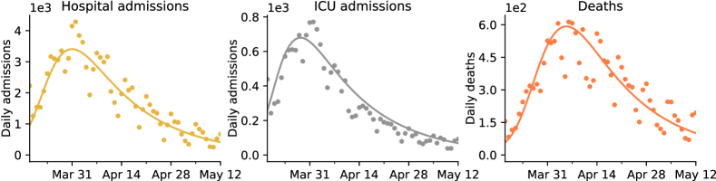
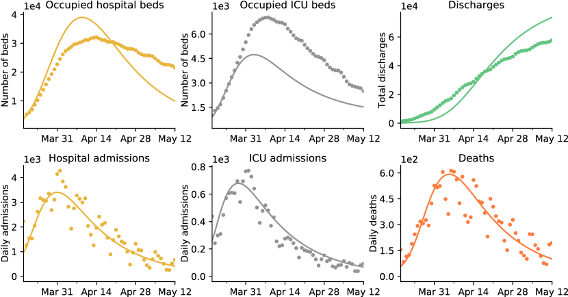
We have fitted this model to the following three time series: daily number of admissions in hospital and ICU, and daily deaths. Fitting such “incidence” time series only requires to estimate the entrance time in each compartment, and not the corresponding sojourn times. The best fitting model is represented in Figure 1, and the inference procedure is described in Section 4. We see that our simple model reproduces quite well the shapes of the three incidence time series. The estimated reproduction number after lockdown is , and that before lockdown is . Thus we estimate that the lockdown yielded a reduction of the reproduction number by a factor . Moreover, the estimated number of infections having occurred before March 18 2020 is . All these estimates are in line with that of other studies on the same dataset [50, 53].
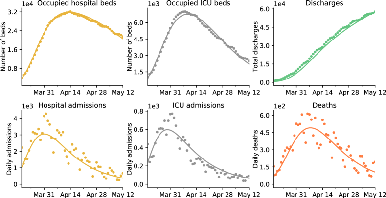
Fitting prevalence data.
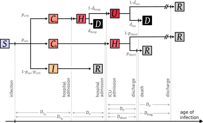
Our second objective is to fit three additional time series: the number of occupied hospital and ICU beds, and the number of discharged individuals. Using the simple admission model only yields a poor fit of these new times series, see Figure 7. We have identified two main causes for this discrepancy. First, we have made the simplifying assumption that individuals are always admitted to ICU prior to death. However, it has been reported that a large fraction of deaths do not involve a preliminary ICU admission [40], and our assumption leads to a fraction of deaths among ICU patients much higher than that previously reported. Second, there are many heterogeneities in the population, such as the (actual) age, that are known to play an important role in the severity of the symptoms of COVID-19 and that are not accounted for.
Thus, we used a more detailed model to reproduce all six time series, which is illustrated in Figure 6 and referred to as the occupancy model. Again, a detailed description of the model and its parameters is available in Section 4.4. The main two differences with the admission model are that a fraction of individuals die shortly after hospital admission, and that we distinguish between individuals who recover fast after their admission and individuals who recover slowly. The best-fitting model is displayed in Figure 2. Again, it reproduces quite well the shapes of all the time-series. Under the occupancy model, the estimated reproduction number after lockdown is and the estimated number of infections before March 17 2020 is . These estimates are close to those obtained under the admission model, indicating that the predictions made by the simple admission model are quite robust to the addition of model details.
Overall, our inference work suggests that a simple model can be used to determine “global” epidemiological parameters, such as the reproduction number and total number of infections, whereas obtaining a prediction for the number of individuals in hospital or ICU requires to use a more detailed model that accounts for population heterogeneity. Moreover, it demonstrates that decorated age-structured models can be readily used to carry out parameter inference in the context of COVID-19, even when the underlying compartment structure is quite complex.
Section 4 contains a detailed description of the inference procedure, as well as a comparison of the various estimates that we obtain with estimates currently available in the literature.
1.6 Connection with ODE models
Section 1.2 shows that the SIR model can be seen as a decorated age-structured model, with well-chosen Markov life-cycle process and Poisson infection point process. This section extends this representation to a broader class of ODE models. We will be interested in solutions to the following set of ODEs:
| (7) | ||||
The parameter gives the rate of new infections from individuals in compartment such that the newly infected individual starts in compartment . The matrix with entries is referred to as the transmission matrix. For , corresponds to transition rate from compartment to compartment . The transition matrix with entries is denoted by , and we further impose that
This class of ODE models encompasses many common epidemic models, including the SIR and SEIR models, as well as all models described in [8, Chapter 4] for instance.
Proposition 3.
- 1.
- 2.
Proof.
By differentiating both sides of (8) w.r.t. time, we obtain
By conditioning on the process and using standard properties of Poisson point processes, we can compute the intensity measure of as
so that
By using the boundary condition of (1) and the fact that is a Markov process with generator we get
from which the first item follows.
It is clear that if then . Fix some and . If , then it can be decomposed as
where is a probability vector and . This decomposition can for instance be recovered from
Consider a Markov process with transition matrix and distributed as . If is such that infections occur at rate when , the first item proves that (7) can be written as (8). ∎
The previous result provides a simple criterion for a system of ODEs to be represented as a decorated age-structured PDE. This criterion has already been proposed previously and is referred to as the “separable mixing” assumption [15, 14]. A direct consequence of this result is that not all ODE models can be represented using a single decorated age-structured PDE. However many models fulfill the requirement that , including models with a single infectious state, those where new infected individuals always start in the same state, and all classical models exposed in [8, Chapter 4]. In that sense, our framework greatly extends the usual systems of ODEs widely used in epidemic modeling.
An important situation where is that of heterogeneous contact rates in the population. For instance, the contact rate could depend heavily on the (actual) age group to which individuals belong, and more contacts are made within the same age class than between classes. A second example is that of spatial heterogeneity, where contacts are more likely to occur between spatially close individuals. It remains possible to derive a representation of (7) in the case using an age-structured model, but this would require to use a multi-dimensional version of (1), which is a straightforward extension of this model.
1.7 Relation with previous works and outline
Deterministic epidemic models where the infectivity depends on the individuals’ age of infection were first introduced in [36], and their mathematical properties have been further studied thoroughly [48, 13, 55], see [30] for a recent account. However, these models have received surprisingly little attention in applications compared to their ODE counterpart, which have been widely used for instance in the context of COVID-19 [49, 50, 19, 12, 17]. In this direction, let us mention [24] which makes use of an epidemic model with memory and [28] were a set of transport PDEs similar to (1) is used. Note that, in contrast with our approach, the PDE in the latter work has two dimensions and is structured according to the time since the entrance in the compartments rather than by infection age. We hope that our work illustrates well the practical potential of such general models. The relation between age-structured and ODE epidemic models exposed in Section 1.2 is known since their very introduction [36], and has been acknowledged multiple times since then [43, 16, 7, 30].
In the most general formulation of a CMJ process, individuals can carry a trait valued in an abstract measure space that encodes all the information about their infection [31, 54]. We have restricted this information to the sequence of compartments visited by each individual, but we could have included some additional details, such as the evolution of the viral load for instance, which could be modeled as a continuous trait following a diffusion. Our result would carry over to the general setting, with a modified limiting equation in Theorem 1 which has already been proposed in [43, Eq. (2.5)] and [44, Chapter IV, Section 1.3]. (Note that none of these works is concerned with the underlying stochastic model.) However, we believe that our current formalism, where the state of an infected individual can be described by a discrete set of compartments, is flexible enough for applications, while being easier to grasp than the general case.
Non-Markov epidemic models have already been investigated, see e.g. [52, 46, 3, 5]. In particular our work shares similarities with a recent series of work in this direction [46, 23, 47]. Let us briefly show how to translate the model in [23] in our framework. Let be some random function giving the infectiousness of a typical individual in the population. Conditional on , let be a time-inhomogeneous Poisson point process with intensity , define
and set
Then, up to the choice of the initial condition and the fact that we make a branching assumption, the model considered in [23] coincides with the model considered here for this specific choice of the pair . (It coincides exactly with the extension of our model considered in [18].)
The main result in [23] shows that the fraction of individuals in each state (, , , and ) converges to the solution of a set of Volterra equations, see their Theorem 2.1. A straightforward computation shows that the latter equations are equivalent to the non-linear version our decorated McKendrick-von Foerster PDE obtained by replacing (5) by (1), with the specific choice of described above.
The idea of representing a general branching population by its age structure has a rich history in probability theory [31, 20, 35, 33, 32, 29, 57, 22] and the connection with the McKendrick-von Foerster PDE has been acknowledged several times [20, 29]. In the latter two works, the authors allow for birth and death rates that may depend not only on abundances of each type, but also on the whole age structure of the population. This impressive level of generalization comes at the cost of assuming that the process describing the evolution of the empirical measure on ages and types is Markovian. In particular, birth and death rates are not allowed to depend on past individual birth events. The Markov property then allows the use of a generator for the empirical measure and with some extra finite second moment assumptions on the intensity measure, this approach allows the authors to obtain a law of large numbers and a central limit theorem.
Even if the current work is not as mathematically challenging as that alluded to above, we believe that our point of view does deserve to be highlighted in the current sanitary crisis since it provides both a general modeling framework and an efficient inference methodology. Furthermore, since we ignore finite population effects, our proofs are quite elementary compared to [20, 29] and should be accessible to a much wider audience interested in such a modeling approach. Finally, as far as we can tell, the duality result exposed in Section 2.4 is new and can presumably be extended to more general branching processes where birth and death rates are allowed to be frequency-dependent. In [18], some of the authors of the present work show that this duality result has a natural counterpart in a model with a finite but large population.
Outline.
The remainder of the paper is organized as follows. Section 2 is devoted to the study of Eq. (5). After providing a formal construction of the branching process that we consider in Section 2.1, the definition of a weak solution to (5) is given in Section 2.2. Then, we derive two probabilistic representations of this solution: we show in Section 2.3 that it corresponds to the first moment of the branching process that we are studying, when viewed as a random measure on the ages of infection; Section 2.4 provides a construction of the weak solution using a dual genealogical process. The two laws of large numbers are proved in Section 3. Finally, Section 4 describes the inference procedure, and compares the estimates that we obtain to known estimates from the literature.
2 Two Feynman-Kac formulæ
2.1 Assumptions and notation
CMJ branching process with suppression.
Recall that the infection process is modeled by a Crump-Mode-Jagers (CMJ) branching process [31, 45] with no death, starting from one individual called the progenitor (or root of the tree). It can be briefly constructed as follows.
Using the Ulam-Harris labeling, the population can be indexed by
The set encodes a tree where is the -th child of . Each individual is characterized by a pair embodying respectively the processes of secondary infection events from and of types carried by . Each pair is an i.i.d. copy of the pair with law , except when is the root, where it is distributed as with law (more on that below).
An infection time can be assigned to all individuals inductively as follows, with the convention that for individuals that are not infected. Suppose that is known (see below). Then, if has been defined, let denote the atoms of in increasing order. That is,
with . Set for , and, independently for each , set
where we recall that is the contact rate. This amounts to trimming the tree by pruning the subtree stemming from with probability , see Figure 3.
Initial shifted law.
In order to connect the distribution of the CMJ to the McKendrick-von Foerster equation, we allow the progenitor to have an initial age with an arbitrary distribution. Let be a r.v. distributed according to some density . Define the infection time of as . The secondary infections induced by the progenitor occur at some times , …, , where are the atoms of a point process defined as
where the pair has law . The point process is obtained from by erasing all atoms that would lead to an infection before . Define , and let be the distribution of . We refer to as the initial shifted law. The infection times are then defined recursively as above, from i.i.d. pairs with the original law .
Assumptions.
The following assumptions will be made implicitly in the remainder of our work. For simplicity, we assume that the contact rate is a piecewise continuous function, and that for any , the process is a.s. continuous at .
Recall that the intensity measure of the point process is denoted by , and implicitly defined as
for any test function , where we used the notation . We assume that has a density w.r.t. the Lebesgue measure that we still denote by , and assume that
We also assume that there exists a unique parameter , the so-called Malthusian parameter of the (untrimmed) CMJ process, such that
| (9) |
The parameter can be either positive (supercritical case) or negative (subcritical case).
2.2 McKendrick-von Foerster PDE: Weak solutions
This section provides the existence and uniqueness of weak solutions to Eq. (5). Even if similar results are well-known for the time-homogeneous McKendrick-von Foerster equation [30, Chapter 1], we derive them briefly here for the sake of completeness.
In order to motivate our definition of weak solutions, we start by giving a well-known formal resolution of the PDE using the method of characteristics. Fix . Let
Then
so that is conserved along the characteristics, i.e.,
It follows that
| (10) |
where
is the number of new infections at time . We now determine the function . Injecting the previous expression into the “age” boundary condition of the PDE, we obtain a convolution equation for : for every
| (11) |
Recall that denotes the Malthusian parameter defined in (9).
Lemma 4.
There exists a unique solution to (11) which is locally integrable. Moreover, for any such that we have , where denotes the set of all functions such that .
Proof.
Fix and let denote the quotient space of by the relation , where if . Then define the linear operator by
Then we have
Now using that
we obtain that . Define
Then is invertible with inverse . Note that equation (11) can be written as
where
Noting that as
proves existence and uniqueness of the solution to (11) in . Now for any two functions and such that and and both satisfy (11), we have (i.e., there is a single element in the equivalence class of verifying (11) for all ). This shows uniqueness of the solution to (11) in .
Since all elements of are locally integrable, this also shows the existence of a locally integrable solution to (11). Its uniqueness can be proved following the exact same reasoning as previously, replacing integrations on by integration on compact intervals. ∎
2.3 A forward Feynman-Kac formula
Consider a CMJ with initial shifted law and define
where is interpreted as the number of infections between and . Recall that guarantees that for all . Finally, is non-decreasing and we denote by the Stieljes measure associated to .
Lemma 6.
There exists a locally integrable function such that
Further, coincides with the unique locally integrable solution of the convolution equation (11).
Proof.
The fact that has a density easily follows from the fact that has a density. The fact that ensures that is locally integrable.
Define the infection measure obtained from after random thinning by the function . Namely, conditional on and the atoms of , we remove independently each of the atoms with respective probabilities , whereas the other atoms remain unchanged.
Fix . Let . Define as the measure obtained from as follows. Conditional on the atoms of , we remove independently each of the atoms with respective probabilities
and leave other atoms unchanged. Note that the thinning procedure is now independent of the starting time . Further, if , the point measure dominates .
We decompose the births on into two parts: individuals stemming from the root and a second part from subsequent births. Using the fact that for every individual , the (un-suppressed) random measure is independent of its birth time (see second equality below), and setting , we get
with . In particular, if , and is a continuity point of , we have . We will pass to the limit in the latter inequality. Recall that is bounded (and valued in ) and right-continuous. The first term on the RHS can be written under the form
where
We will now apply twice the Bounded Convergence Theorem. On the one hand, for a fixed value of , as
Further, the latter term (i.e., the integrand in the integral defining ) is uniformly bounded by and . A first application of the Bounded Convergence Theorem implies that for every , as
On the other hand, the uniform bound, for all , allows us to again apply the Bounded Convergence Theorem, so we get
By replacing the by a and using a similar argument, one can establish the same lower bound and strengthen the latter inequality into an equality. A simple change of variable and interchanging the order of integration yields
Finally, differentiating with respect to yields the desired result. ∎
Corollary 7 (Forward Feynman-Kac formula).
For every , define
where is the unique weak solution to the McKendrick-von Foerster PDE with initial condition . Then
| (12) |
where the expected value is taken with respect to a CMJ process starting with one individual with infection and life-process distributed according to the shifted law .
Proof.
Define
We need to check that on the space of finite measures. Let be a non-negative, bounded, continuous function on and a non-negative, continuous function with compact support in . As in the previous lemma, we have
Let be the first term on the RHS. For every
By reasoning along the same lines as in Lemma 6 (i.e., applying the Bounded Convergence Theorem several times), one can show that the RHS converges to
as and thus
By a similar argument, the inequality can be strengthened into an equality. After some simple changes of variables we get
Moreover we have
so that
It is easy to check that the two functions and are both continuous. As a consequence, we have for every test function , concluding the proof. ∎
2.4 Dual CMJ process and backward Feynman-Kac formula
We end this section by making a connection between a dual process – interpreted as an ancestral process – and the (PDE) method of characteristics. In addition, this approach provides a probabilistic proof of uniqueness for the PDE.
Let be any random point measure with intensity measure . Fix . We now construct a dual process using the measure , which can be seen as a generalized Bellman-Harris branching process (individuals have a finite lifetimes, births only occur upon death). Let us first describe the process with no suppression (i.e., ).
-
•
Start with a single particle at time . Assume that the residual lifetime of this original particle is , so that this particle dies out at time .
-
•
As in a Bellman-Harris process, the number of offspring of an individual and their lifetime durations are independent of the parent’s characteristics.
-
•
Upon death, each individual is endowed with an independent copy of : the number of offspring of is given by the number of atoms of and their lifetime durations are given by the positions of the atoms in .
The dual process with suppression can be coupled with the case . Given a realization of the process, if a branching occurs at time , the children are killed independently with probability . (Note that as in the original CMJ process, suppression translates into trimming the dual tree.)
Remark 4.
We note that there are as many dual processes as there are point processes with intensity measure . Here are a few natural choices:
-
1.
Take .
-
2.
Let be a Poisson Point Process with intensity measure . In this particular case, the dual process is a Bellman-Harris branching process (i.e., the offspring lifetime durations are independent conditional on offspring number). We note that appears naturally when considering the ancestral spine of a critical CMJ, see e.g. [51]. The measure can be obtained by size-biasing (i.e. biasing by the total mass of ) and then recording the age of the individual at a uniformly chosen birth event.
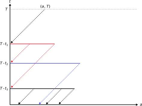
Let be the stochastic process valued in recording the residual life-times at time listed in increasing order, i.e. if there are particles alive at time and is the residual life-time of the -th individual with . (We assumed that has a density so that the residual lifetimes are distinct a.s.) In particular, the particle labelled at any given time will be the first to expire, and at death time a random number of children is produced. We let denote the number of particules alive at time , i.e., the dimension of the vector .
Proposition 8 (Backward Feynman-Kac formula).
For any probability density , we have
| (13) |
where is the unique solution to the McKendrick-von Foerster equation started from , and is the distribution of the process starting with an individual with residual lifetime .
Proof.
Let be the successive branching times of the dual branching process. Since has a density, there is a single branching particle at the successive branching times Define the process
See also Figure 4 for a pictorial representation of the process. It is plain from the definition that is preserved along the characteristics of the PDE, i.e., that for every the function remains constant on . As a consequence, remains constant on every interval , with the convention . Define the value of the process at the -th branching time. Let be the filtration induced by the process . By definition of the dual process, we have
For every
where the third equality follows from the age boundary of the McKendrick-von Foerster equation, and the last equality from the identity . As already mentioned, the process is constant between two branching times. As a consequence, is a martingale (w.r.t. its natural fltration) so for every ,
Relation (13) follows by taking in the latter expression. ∎
3 Proofs of the main results
In this section, we provide the proofs of the two laws of large numbers stated in Section 1.4. The proof of Theorem 1 is a direct consequence of the results of the previous section.
Proof of Theorem 1.
Recall the definition of the empirical measure . It can be written as
| (14) |
where are independent copies of . Let be an arbitrary continuous and bounded function on . The law of large numbers combined with Corollary 7 implies that
which ends the proof. ∎
We now turn our attention to the proof of Theorem 2, the law of large number started from a single individual. Let us briefly recall the setting of this result.
We consider a sequence of random times with a.s. on the non-extinction event. We assume that the process starts from a single individual infected at time and that the contact rate of the CMJ depends on in the following way: , where is a piecewise continuous function in such that for all .
Proof of Theorem 2.
The result will follow by viewing the population at time as an adequate random characteristic of the population at time . Let us recall some basic facts about random characteristics of CMJ processes in our context. We refer to [35, 54] for a more thorough account on this notion.
We consider a plain CMJ with no contact rate or initial shifted law. Every individual is characterized by an independent pair of random variables . A random characteristic is a real-valued stochastic process that can be constructed from the collection . (More formally it is a càdlàg process measurable w.r.t. the -field induced by these variables.) By convention, it is extended to a process defined on the whole real line by setting for .
For an individual let us write for the random characteristic constructed from the collection . It is the characteristic constructed from the tree rooted at of all descendants of . The branching process counted by the random characteristic is then defined as
We now recall one of the main results of Jagers and Nerman [34], namely Theorem 5.8 (see also Theorem 4, Appendix A in [54]). Recall that denotes the Malthusian parameter defined in (9). On top of all the assumptions above, we make the two following extra assumptions
-
(a)
The characteristic fulfills
-
(b)
The map is continuous a.e. with respect to the Lebesgue measure.
Then there exists a positive r.v. (independent of the choice of ) such that conditional on non-extinction
To illustrate the method, we recall that if we take then coincides with , the total number of births before time . For this particular choice of (deterministic) characteristic, the two properties above are immediately satisfied (recall that ), so that conditional on non-extinction
This convergence ensures that the first item of our theorem is satisfied.
To prove the second item, let us set
for the atoms of the infection point process of the ancestor . Further denote by the empirical measure of ages and compartments at time of the progeny of the -th child of the ancestor, thinned by the contact rate , i.e.,
where refers to the infection time of once the tree has been thinned. (That is, if remains infected after the thinning, or otherwise.) Our characteristic of interest can now be defined as
for a fixed time and a fixed bounded continuous function . On the one hand, it should be clear that
| (15) |
To see this, note that the process is obtained from a plain CMJ with no thinning, so that only infections after time are removed due to the contact rate.
On the other hand, can be obtained by starting from an initial individual with age , removing all atoms from its infection point process before time , and integrating the empirical measure of the resulting CMJ at time against . This is the description of the CMJ with initial shifted law conditional on , so that
| (16) |
where in the age of the initial ancestor is distributed according to .
Therefore, up to checking (a) and (b), Theorem 5.8 in [35] shows that, as ,
in probability, which in combination with (16) proves the result.
All what remains to be shown is that (a) and (b) are fulfilled. That is continuous a.e. follows directly from the fact that has a density. Condition (b) is a consequence of the following stochastic domination
where are i.i.d. copies of the CMJ without thinning, independent of . ∎
4 Inference procedure
In this section, we illustrate how to use our framework to make inferences from macroscopic observables of the epidemic, e.g., incidence of positively tested patients, hospital or ICU (intensive care unit) admissions, deaths, etc. We show how to use those observables to extract the underlying age structure of the population, estimate model parameters, and forecast the future of the epidemic.
We focused on a longitudinal case study in France. From March 18 2020, the French government has provided daily reports of the numbers of ICU and hospital admissions, of deaths, of discharged patients, and of occupied ICU and hospital beds. Moreover, several theoretical studies have already been conducted on the same dataset. This allowed us to fix the values of some crucial biological parameters that had already been estimated and to carry out a comparison with our method. We want to emphasize that the aim of this section is to provide a mathematical framework in which convergence results can be rigorously proved while remaining flexible enough for other applications. Our goal is not to provide new estimates of epidemiological parameters for France, as many robust estimates are already available. For instance we do not provide confidence intervals for our estimates, and neither do we conduct a sensibility analysis.
The remainder of the section is laid out as follows. In Section 4.1 we identify the mathematical quantities that impact the dynamics of the epidemic for large population sizes, and show how to turn them into a likelihood. Section 4.2 then presents the choice of distribution we made for these quantities and the parameters that need to be estimated. Finally, estimation of these parameters from the French incidence data is performed in Section 4.3 and Section 4.4. We start by fitting a simple model in Section 4.3 and then show how this model can be made more complex to account for more complex data in Section 4.4.
4.1 Deriving the likelihood
Under the assumptions of Theorem 2, the number of individuals in a given state at time converges to
| (17) |
where is the solution to (5). The required assumptions are in essence that the epidemic has been ongoing for a long enough time at the lockdown onset for the infected population to be large, which we assume to hold true for France as the number of cases on March 16 2020 was on the order of thousands of individuals.
Therefore, we take (17) as the predicted number of individuals in state in our model. In order to turn (17) into a likelihood, we assume that the observed number of individuals in state at time is distributed according to some discrete law centered on the predicted value, which we take to be a Poisson distribution. Then, the likelihood for the whole time period is obtained by assuming that the observations are independent across states and time. The explicit expression for the likelihood is provided in Section A.3.
Remark 5.
The assumption that observations are independent is obviously not met. For instance, the number of occupied hospital beds is cumulative, so that any error is propagated from one day to the other. Moreover, there is a clear weekly effect in data that is not accounted for here. As deriving robust estimates is not the main purpose of this work, we prefer to keep this independence assumption that leads to simple expressions for the likelihood, while being aware of its limitation. This assumption could be relaxed by modeling explicitly the observation process and its potential errors.
Remark 6.
We have decided to use an expression for the likelihood similar to that in [50, 53]. Such an expression only poorly accounts for the deviation of the stochastic model from its deterministic limit. Better accounting for this effect would require to use the likelihood of the stochastic model, or a Gaussian approximation of it obtained by deriving a functional central limit theorem. In our context the covariance structure of the population could be obtained by adapting the expressions in [34, Section 3] to incorporate the contact rate . However the resulting expressions would be quite cumbersome and computationally costly so that we prefer to use our simpler Poisson likelihood.
Under our assumptions, the likelihood only depends on (17), which is in turn determined by four quantities that need to be parametrized:
-
1.
The intensity measure of the infection point process .
-
2.
The initial number of infected individuals and their age profile.
-
3.
The contact rate after lockdown .
-
4.
The one-dimensional marginals of the life-cycle process for .
4.2 Parametrization of the model
Average infection measure.
Recall the definition of and from Section 2.1 and further define
The total mass of , , corresponds to the mean number of secondary infections induced by a single infected individual if . Thus is the basic reproduction number at the start of the epidemic, when no control measure is enforced. In order to distinguish it from the reproduction number during lockdown, it will be denoted by . We leave it as a parameter to infer.
The function is the density of a probability measure known as the generation time distribution [59, 9]. This distribution has been estimated shortly after the epidemic onset by several studies [21, 27, 10]. We use the estimation of [21], and assume that is a Weibull distribution, that is
| (18) |
where the values of the shape parameter and scale parameter are recalled in Table 1.
Initial condition.
According to Theorem 2, the initial age structure of the population is
where is the Malthusian parameter of the epidemic prior to implementation of control measures, and is the number of infected individuals at , that is, at the lockdown onset. The parameter corresponds to the exponential growth rate of any observable of the epidemic during this period. We chose to estimate it from the cumulative number of deaths, which appeared to be more reliable than the number of detected cases as the number of tests conducted in the early phase of the epidemic in France varied greatly. It was estimated using a linear regression on the logarithm of the number of deaths from March 7 to March 20 2020, and the corresponding basic reproduction number before lockdown, , was computed using the Euler-Lotka equation (9) assuming that the generation time distribution is given by (18). Both estimates are shown in Table 1.
| Notation | Description | Value | Source |
|---|---|---|---|
| Pre-lockdown exponential growth rate | 0.315 | E | |
| Basic reproduction number before lockdown | 3.25 | E | |
| Shape parameter of the generation time | 2.83 | [21] | |
| Scale parameter of the generation time | 5.67 | [21] |
Contact rate.
The contact rate accounts for the temporal variations in transmissions after the lockdown onset. As we focus on the period from March to May 2020 where no additional control measure has been enforced in France, we will assume that is constant and denote by its value, that is, . The reproduction number after the lockdown is denoted by .
Life-cycle.
The last quantities that need to be defined are the one-dimensional marginals of the life-cycle process . These could be directly estimated from hospital patient pathways as in [41, 58, 40]. However, when such data is not available they need to be estimated from individual counts in each compartment. In this case, we propose the following parametrization of the process based on Gamma-distributed sojourn times.
Let us denote by the sequence of states visited by . We assume that is a Markov chain on , and that it ends either in a “dead” or “recovered” state, that are assumed to be absorbing.
For , the sojourn time in is supposed to be Gamma-distributed with mean and variance , for some global dispersion parameter shared across all states. More precisely, let denote the sequence of sojourn times of , that is, is the sojourn time in state . We assume that conditional on , the variables are independent. Moreover, if , then follows a Gamma distribution with mean and variance , that is,
Thus, the one-dimensional marginals are parametrized by the transitions of a Markov chain on , as well as by one parameter for each , and a global parameter . Under this parametrization the one-dimensional marginals can be efficiently computed, while only requiring one parameter for the sojourn time in each state. Two concrete examples of Markov chains are discussed in the next sections.
4.3 Inference with the admission model
The first model that we consider, the admission model, is a parsimonious model designed to obtain estimates of the reproduction number during lockdown, and of the number of infections in France in early March. It is illustrated in Figure 5. We fit it to the three “incidence” time series: the daily number of admissions in hospital and ICU, and the daily number of deaths.
Description of the model.
Upon infection, with probability , an individual develops a mild form of COVID-19 and is placed in state , which encompasses all cases that do not require a hospitalization. With probability the individual has a severe infection and is placed in state . Individuals in state are eventually hospitalized and moved to state . Then, with probability individuals in state are admitted in ICU and moved to state . Otherwise they eventually recover and are discharged. Finally, individuals in state die with probability , or recover with probability . In this model, only individuals in ICU may die.
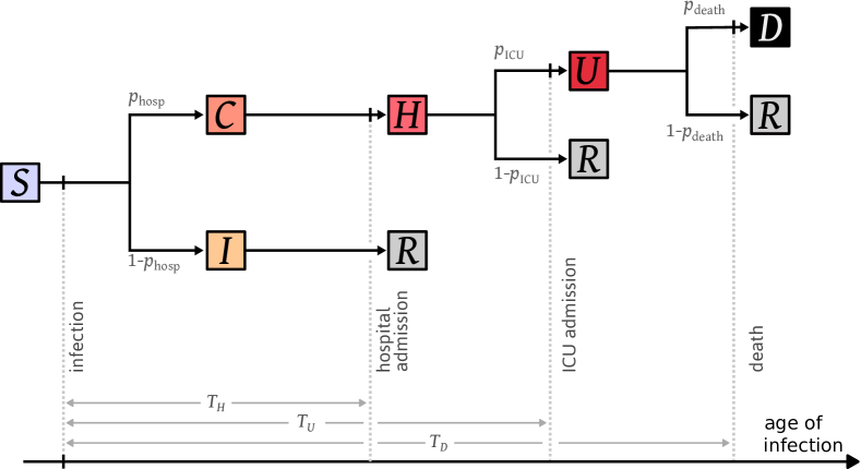
As we are fitting the number of individuals that enter a state, and not the number of individuals that are currently in that state, we only need to track the times , , and elapsed between infection and hospital admission, ICU admission, and death, respectively.
Inference results.
Estimations of , and of the death probability conditional on hospitalization (equal in our setting to ) in France have already been conducted in [50]. We used these estimates and considered the values of , , and as fixed. All other parameters were estimated using a maximum likelihood procedure described in Section A.3. The parameter estimations are provided in Table 2, and the corresponding predicted values for the time series under consideration are displayed in Figure 1. Overall, our simple model seems to match the observed data. Note however that the model overestimates the number of ICU admissions in the second part of the lockdown. This is likely due to a temporal reduction in the ICU admission probability which has been reported in [50].
Our estimation of the basic reproduction number during the lockdown period is . This suggests that lockdown has reduced the basic reproduction number by a factor compared to the beginning of the epidemic. Moreover, we estimated that infections have occurred in France before March 17. Both these values are in line with previous estimates for France [53, 50].
We did not impose that in the inference procedure. Interestingly we found that the data are best explained by assuming that the mean of is days, whereas the mean of is days. This indicates that the delay between infection and hospital admission is shorter for individuals that end up in ICU, compared to the average time between infection and hospitalization. Therefore it would be more appropriate to allow individuals to have an admission to hospital delay that is different depending on whether they will end up in ICU or not, modeling the fact that they have a more severe form of the disease. We estimated the mean of , the time between infection and death, to be days. This estimate is lower than but consistent with previous estimates based on the study of individual-case data [60, 41, 58].
| Notation | Description | Value | Source |
|---|---|---|---|
| Reproduction number during lockdown | E | ||
| Total number of infections before March 17 2020 | E | ||
| Probability of being hospitalized | [50] | ||
| Probability of entering ICU conditional on being at the hospital | [50] | ||
| Death probability conditional on being hospitalized | [50] | ||
| Delay between infection and hospital admission | days | E | |
| Delay between infection and ICU admission | days | E | |
| Delay between infection and death | days | E | |
| Scale parameter common to all Gamma distributions | 0.463 | E |
4.4 Inference with the occupancy model
We now consider a model aimed at providing predictions for the number of hospitalized individuals and ICU patients. The model is fitted to the three “incidence” time-series, and to three additional “prevalence” time-series: the number of occupied hospital and ICU beds, and the number of discharged hospital patients.
A first attempt to fit the prevalence curves could be to keep the admission model of Figure 5 and to estimate the time between hospital admission and discharge using the observed number of occupied ICU, hospital beds, and discharged patients. However this only yields a poor fit of the data (see Section A.4). We identified two main reasons for this discrepancy. First, we assumed that all individuals are admitted to ICU prior to death. Using the probability estimated in [50] then yields that the probability of dying conditional on being in ICU is . This value is unrealistically high, and we need to assume that a fraction of hospital deaths occur without going through the ICU. Second, under the admission model, the delay between hospital admission and discharge is almost unimodal. However, the observed number of occupied hospital beds rises fast but falls slowly. Such a shape cannot be easily accounted for by a unimodal distribution for the time spent in hospital.
Description of the model.
Taking into account the previous two points required us to make the model more complex. The resulting model, referred to as the occupancy model, is illustrated in Figure 6. We now consider that upon infection, individuals go to one of three states depending on the severity of their infection:
-
•
The state which gathers critical infections that lead to death or ICU admission. The probability of having a critical infection is denoted by .
-
•
The state which corresponds to severe infections that require a hospitalization but are not critical. Such infections occur with probability .
-
•
The state which consists of all mild infections that do not lead to a hospital admission, and occur with probability .
Individuals in state are admitted to hospital after a duration . Then, with probability they are discharged after a duration , while with probability they are discharged after a duration .
Critically infected individuals are admitted to hospital after a duration . Upon arrival at hospital, they die immediately with probability , or go to ICU after a duration . Individuals in ICU die with probability after a delay . Otherwise they are discharged after a stay of length .
Inference results.
In our model, the probability of hospital admission is , the probability of ICU admission is and that of death is . We have fixed these three values to those estimated in [50], and we only had one remaining parameter out of 4 (, , , ) to estimate from the data. We have fixed the time to days as estimated in [50]. All other parameters were estimated using a maximum likelihood method described in Section A.3. The estimated parameter set is shown in Table 3, while Figure 2 shows the best-fitting model.
The estimated parameters provide a good fit of the six observed time series. Again, the model has a tendency to overestimate the ICU admissions in the second part of the lockdown, which has the same interpretation as for the admission model.
Under the occupancy model, we estimated that , and . These estimates are extremely close to those made with the admission model. The estimated mean time between infection and death or hospital, ICU admission are respectively days, days and days. Again we see that these estimates in the more complex model are consistent with those of the simple model. The mean recovery time from hospital is days for severe infections, and days for critical infections. This yields an overall mean recovery time of days. Finally, we estimated that the death probability conditional on being in ICU is . This yields that in our model a fraction of all deaths occur shortly after hospital admission. This result is consistent with [50] that estimated that a fraction of all deaths occurred within the first day after hospital admission. However, it has been reported in [25] that the death probability of ICU patients is . Our estimated value is thus unrealistically high. This indicates that there is a fraction of hospital deaths that occur without any ICU admission, and not quickly after hospital admission, that our model is not accounting for.
| Notation | Description | Value | Source |
|---|---|---|---|
| Reproduction number during lockdown | E | ||
| Total number of infections before March 17 2020 | E | ||
| Probability of being hospitalized | [50] | ||
| Probability of entering ICU conditional on being at the hospital | [50] | ||
| Death probability conditional on being hospitalized | [50] | ||
| Probability of death conditional on being in ICU | E | ||
| Probability of a short stay at hospital | E | ||
| Delay between severe infection and hospital admission | days | E | |
| Delay between hospital admission and quick discharge | days | E | |
| Delay between hospital admission and slow discharge | days | E | |
| Delay between critical infection and hospital admission | days | E | |
| Delay between hospital admission and ICU admission | days | [50] | |
| Delay between ICU admission and discharge | days | E | |
| Delay between ICU admission and death | days | E | |
| Scale parameter common to all Gamma distributions | E |
Our estimates, though they are not the key message of the present paper, can nevertheless draw attention to potential heterogeneities in the infected population. We estimated that the mean time between infection and ICU admission is shorter than that between infection and hospital admission. This suggests that the time between infection and severe symptom onset is shorter for critical infection, that lead to ICU admission, than for milder ones. Moreover, fitting the prevalence time series required to divide the hospital and death compartments in two subcompartments, indicating that the data are not well explained by a simple homogeneous model, as seen in Figure 7. Such heterogeneity could originate from underlying structuring variables, such as comorbidity or (actual) age, that we are not accounting for. Many estimates of clinical features, such as the incubation period, are obtained from a pooled dataset that does not take heterogeneity in the population into account [1, 41, 39, 56, 6, 42, 17]. When estimating the total number of infected individuals using only a fraction of the detected cases, e.g., using the hospital admissions or deaths, it is interesting to keep in mind that the time periods estimated from pooled studies could be inaccurate for the fraction of infected individuals under consideration.
Acknowledgements
The authors thank the Center for Interdisciplinary Research in Biology (CIRB) for funding and the taskforce MODCOV19 of the INSMI (CNRS) for their technical/scientific support during the epidemic. P.C. has received funding from the European Union’s Horizon 2020 research and innovation program under the Marie Skłodowska-Curie grant agreement PolyPath 844369.
References
- [1] Jantien A. Backer, Don Klinkenberg, and Jacco Wallinga. Incubation period of 2019 novel coronavirus (2019-nCoV) infections among travellers from Wuhan, China, 20–28 January 2020. Eurosurveillance, 25(5), 2020.
- [2] J. Baker, P. Chigansky, K. Hamza, and F. C. Klebaner. Persistence of small noise and random initial conditions. Advances in Applied Probability, 50(A):67–81, 2018.
- [3] Frank Ball. A unified approach to the distribution of total size and total area under the trajectory of infectives in epidemic models. Advances in Applied Probability, 18:289–310, 1986.
- [4] A. D. Barbour, P. Chigansky, and F. C. Klebaner. On the emergence of random initial conditions in fluid limits. Journal of Applied Probability, 53:1193–1205, 2016.
- [5] Andrew D Barbour. The duration of the closed stochastic epidemic. Biometrika, 62:477–482, 1975.
- [6] Qifang Bi, Yongsheng Wu, Shujiang Mei, Chenfei Ye, Xuan Zou, Zhen Zhang, Xiaojian Liu, Lan Wei, Shaun A. Truelove, Tong Zhang, Wei Gao, Cong Cheng, Xiujuan Tang, Xiaoliang Wu, Yu Wu, Binbin Sun, Suli Huang, Yu Sun, Juncen Zhang, Ting Ma, Justin Lessler, and Tiejian Feng. Epidemiology and transmission of covid-19 in 391 cases and 1286 of their close contacts in shenzhen, china: a retrospective cohort study. The Lancet Infectious Diseases, 20:911–919, 2020.
- [7] Fred Brauer. The Kermack–McKendrick epidemic model revisited. Mathematical Biosciences, 198:119–131, 2005.
- [8] Fred Brauer, Carlos Castillo-Chavez, and Zhilan Feng. Mathematical Models in Epidemiology. Texts in Applied Mathematics. Springer-Verlag New York, 2019.
- [9] Tom Britton and Gianpaolo Scalia Tomba. Estimation in emerging epidemics: biases and remedies. Journal of The Royal Society Interface, 16:20180670, 2019.
- [10] Danilo Cereda, Mattia Manica, Marcello Tirani, Francesca Rovida, Vittorio Demicheli, Marco Ajelli, Piero Poletti, Filippo Trentini, Giorgio Guzzetta, Valentina Marziano, Raffaella Piccarreta, Antonio Barone, Michele Magoni, Silvia Deandrea, Giulio Diurno, Massimo Lombardo, Marino Faccini, Angelo Pan, Raffaele Bruno, Elena Pariani, Giacomo Grasselli, Alessandra Piatti, Maria Gramegna, Fausto Baldanti, Alessia Melegaro, and Stefano Merler. The early phase of the COVID-19 epidemic in Lombardy, Italy. Epidemics, 37:100528, 2021.
- [11] Dorothy H. Crawford. Deadly companions: how microbes shaped our history. Oxford University Press, second edition, 2018.
- [12] Laura Di Domenico, Giulia Pullano, Chiara E. Sabbatini, Pierre-Yves Boëlle, and Vittoria Colizza. Impact of lockdown on COVID-19 epidemic in île-de-france and possible exit strategies. BMC Medicine, 18:240, 2020.
- [13] Odo Diekmann. Limiting behaviour in an epidemic model. Nonlinear Analysis: Theory, Methods & Applications, 1:459–470, 1977.
- [14] Odo Diekmann, Hans Heesterbeek, and Tom Britton. Mathematical Tools for Understanding Infectious Disease Dynamics. Princeton Series in Theoretical and Computational Biology. Princeton University Press, 2013.
- [15] Odo Diekmann, J. A. P. Heesterbeek, and J. A. J. Metz. On the definition and the computation of the basic reproduction ratio in models for infectious diseases in heterogeneous populations. Journal of Mathematical Biology, 28:365–382, 1990.
- [16] Odo Diekmann, J.A.J. Metz, and J.A.P. Heesterbeek. The legacy of Kermack and McKendrick. In D. Mollison, editor, Epidemic Models: Their Structure and Relation to Data. Cambridge University Press, Cambridge, 1995.
- [17] R. Djidjou-Demasse, Y. Michalakis, M. Choisy, M. T. Sofonea, and S. Alizon. Optimal covid-19 epidemic control until vaccine deployment. medRxiv, 2020.
- [18] Jean-Jil Duchamps, Félix Foutel-Rodier, and Emmanuel Schertzer. General epidemiological models: Law of large numbers and contact tracing. 2021.
- [19] Theodoros Evgeniou, Mathilde Fekom, Anton Ovchinnikov, Raphael Porcher, Camille Pouchol, and Nicolas Vayatis. Epidemic models for personalised COVID-19 isolation and exit policies using clinical risk predictions. Production and Operations Management, Special Issue on Managing Pandemics: A POM Perspective, 2021.
- [20] Jie Yen Fan, Kais Hamza, Peter Jagers, and Fima Klebaner. Convergence of the age structure of general schemes of population processes. Bernoulli, 26:893–926, 2020.
- [21] Luca Ferretti, Chris Wymant, Michelle Kendall, Lele Zhao, Anel Nurtay, Lucie Abeler-Dörner, Michael Parker, David Bonsall, and Christophe Fraser. Quantifying SARS-CoV-2 transmission suggests epidemic control with digital contact tracing. Science, 368(6491), 2020.
- [22] Régis Ferrière and Viet Chi Tran. Stochastic and deterministic models for age-structured populations with genetically variable traits. ESAIM: Proc., 27:289–310, 2009.
- [23] Raphaël Forien, Guodong Pang, and Étienne Pardoux. Epidemic models with varying infectivity. SIAM Journal on Applied Mathematics, 81:1893–1930, 2021.
- [24] Raphaël Forien, Guodong Pang, and Étienne Pardoux. Estimating the state of the COVID-19 epidemic in France using a model with memory. Royal Society Open Science, 8:202327, 2021.
- [25] Santé Publique France. COVID-19 : point épidémiologique du 4 juin 2020, 2020.
- [26] Santé Publique France. Données hospitalières relatives à l’épidémie de COVID-19, 2020.
- [27] Tapiwa Ganyani, Cécile Kremer, Dongxuan Chen, Andrea Torneri, Christel Faes, Jacco Wallinga, and Niel Hens. Estimating the generation interval for coronavirus disease (COVID-19) based on symptom onset data, March 2020. Eurosurveillance, 25, 2020.
- [28] Stéphane Gaubert, Marianne Akian, Xavier Allamigeon, Marin Boyet, Baptiste Colin, Théotime Grohens, Laurent Massoulié, David P. Parsons, Frédéric Adnet, Érick Chanzy, Laurent Goix, Frédéric Lapostolle, Éric Lecarpentier, Christophe Leroy, Thomas Loeb, Jean-Sébastien Marx, Caroline Télion, Laurent Tréluyer, and Pierre Carli. Understanding and monitoring the evolution of the Covid-19 epidemic from medical emergency calls: the example of the Paris area. Comptes Rendus. Mathématique, 358:843–875, 2020.
- [29] Kais Hamza, Peter Jagers, and Fima C Klebaner. The age structure of population-dependent general branching processes in environments with a high carrying capacity. Proceedings of the Steklov Institute of Mathematics, 282:90–105, 2013.
- [30] Hisashi Inaba. Age-Structured Population Dynamics in Demography and Epidemiology. Springer Singapore, Singapore, 2017.
- [31] Peter Jagers. Branching processes with biological applications. Wiley, 1975.
- [32] Peter Jagers and Fima C Klebaner. Population-size-dependent and age-dependent branching processes. Stochastic Processes and their Applications, 87(2):235–254, 2000.
- [33] Peter Jagers and Fima C Klebaner. Population-size-dependent, age-structured branching processes linger around their carrying capacity. Journal of Applied Probability, 48:249–260, 2011.
- [34] Peter Jagers and Olle Nerman. The growth and composition of branching populations. Advances in Applied Probability, 16:221–259, 1984.
- [35] Peter Jagers and Olle Nerman. Limit theorems for sums determined by branching and other exponentially growing processes. Stochastic Processes and their Applications, 17:47–71, 1984.
- [36] William O. Kermack and Anderson G. McKendrick. A contribution to the mathematical theory of epidemics. Proceedings of the Royal Society of London. Series A, Containing Papers of a Mathematical and Physical Character, 115(772):700–721, 1927.
- [37] Mi-Young Kim. Long-time stability of numerical solutions to Gurtin–MacCamy equations by method of characteristics. Applied Mathematics and Computation, 176:552–562, 2006.
- [38] H. Krauss. Zoonoses : infectious diseases transmissible from animals to humans. ASM Press, 2003.
- [39] Stephen A Lauer, Kyra H Grantz, Qifang Bi, Forrest K Jones, Qulu Zheng, Hannah R Meredith, Andrew S Azman, Nicholas G Reich, and Justin Lessler. The incubation period of coronavirus disease 2019 (COVID-19) from publicly reported confirmed cases: estimation and application. Annals of internal medicine, 172:577–582, 2020.
- [40] Noémie Lefrancq, Juliette Paireau, Nathanaël Hozé, Noémie Courtejoie, Yazdan Yazdanpanah, Lila Bouadma, Pierre-Yves Boëlle, Fanny Chereau, Henrik Salje, and Simon Cauchemez. Evolution of outcomes for patients hospitalised during the first 9 months of the SARS-CoV-2 pandemic in France: A retrospective national surveillance data analysis. The Lancet Regional Health - Europe, 5:100087, 2021.
- [41] Natalie M. Linton, Tetsuro Kobayashi, Yichi Yang, Katsuma Hayashi, Andrei R. Akhmetzhanov, Sung-mok Jung, Baoyin Yuan, Ryo Kinoshita, and Hiroshi Nishiura. Incubation period and other epidemiological characteristics of 2019 novel coronavirus infections with right truncation: A statistical analysis of publicly available case data. Journal of Clinical Medicine, page 538, 2020.
- [42] Clément Massonnaud, Jonathan Roux, and Pascal Crépey. COVID-19: Forecasting short term hospital needs in France. medRxiv, 2020.
- [43] J. A. J. Metz. The epidemic in a closed population with all susceptibles equally vulnerable; some results for large susceptible populations and small initial infections. Acta Biotheoretica, 27:75–123, 1978.
- [44] J. A. J. Metz and Odo Diekmann. The Dynamics of Physiologically Structured Populations. Lecture Notes in Biomathematics. Springer, Berlin, Heidelberg, 1986.
- [45] Olle Nerman. On the convergence of supercritical general (C-M-J) branching processes. Zeitschrift für Wahrscheinlichkeitstheorie und Verwandte Gebiete, 57:365–395, 1981.
- [46] Guodong Pang and Etienne Pardoux. Functional limit theorems for non-Markovian epidemic models. 2020.
- [47] Guodong Pang and Etienne Pardoux. Functional law of large numbers and pdes for epidemic models with infection-age dependent infectivity. 2021.
- [48] Joannes Reddingius. Notes on the mathematical theory of epidemics. Acta Biotheoretica, 20:125–157, 1971.
- [49] Lionel Roques, Etienne K Klein, Julien Papaix, Antoine Sar, and Samuel Soubeyrand. Using early data to estimate the actual infection fatality ratio from COVID-19 in France. Biology, 9:97, 2020.
- [50] Henrik Salje, Cécile Tran Kiem, Noémie Lefrancq, Noémie Courtejoie, Paolo Bosetti, Juliette Paireau, Alessio Andronico, Nathanaël Hozé, Jehanne Richet, Claire-Lise Dubost, Yann Le Strat, Justin Lessler, Daniel Levy-Bruhl, Arnaud Fontanet, Lulla Opatowski, Pierre-Yves Boelle, and Simon Cauchemez. Estimating the burden of SARS-CoV-2 in France. Science, 369(6500):208–211, 2020.
- [51] Emmanuel Schertzer and Florian Simatos. Height and contour processes of Crump-Mode-Jagers forests (I): general distribution and scaling limits in the case of short edges. Electronic Journal of Probability, 23:43pp., 2018.
- [52] Thomas Sellke. On the asymptotic distribution of the size of a stochastic epidemic. Journal of Applied Probability, 20:390–394, 1983.
- [53] Mircea T. Sofonea, Bastien Reyné, Baptiste Elie, Ramsès Djidjou-Demasse, Christian Selinger, Yannis Michalakis, and Samuel Alizon. Memory is key in capturing covid-19 epidemiological dynamics. Epidemics, 35:100459, 2021.
- [54] Ziad Taïb. Branching Processes and Neutral Evolution, volume 93 of Lecture Notes in Biomathematics. Springer Berlin Heidelberg, Berlin, Heidelberg, 1992.
- [55] Horst R. Thieme. Renewal theorems for some mathematical models in epidemiology. Journal of Integral Equations, 8(3):185–216, 1985.
- [56] Lauren C Tindale, Jessica E Stockdale, Michelle Coombe, Emma S Garlock, Wing Yin Venus Lau, Manu Saraswat, Louxin Zhang, Dongxuan Chen, Jacco Wallinga, and Caroline Colijn. Evidence for transmission of covid-19 prior to symptom onset. eLife, 9:e57149, 2020.
- [57] Viet Chi Tran. Large population limit and time behaviour of a stochastic particle model describing an age-structured population. ESAIM: Probability and Statistics, 12:345–386, 2008.
- [58] Robert Verity, Lucy C. Okell, Ilaria Dorigatti, Peter Winskill, Charles Whittaker, Natsuko Imai, Gina Cuomo-Dannenburg, Hayley Thompson, Patrick G. T. Walker, Han Fu, Amy Dighe, Jamie T. Griffin, Marc Baguelin, Sangeeta Bhatia, Adhiratha Boonyasiri, Anne Cori, Zulma Cucunubá, Rich FitzJohn, Katy Gaythorpe, Will Green, Arran Hamlet, Wes Hinsley, Daniel Laydon, Gemma Nedjati-Gilani, Steven Riley, Sabine van Elsland, Erik Volz, Haowei Wang, Yuanrong Wang, Xiaoyue Xi, Christl A. Donnelly, Azra C. Ghani, and Neil M. Ferguson. Estimates of the severity of coronavirus disease 2019: a model-based analysis. The Lancet Infectious Diseases, 20:669–677, 2020.
- [59] Jacco Wallinga and Marc Lipsitch. How generation intervals shape the relationship between growth rates and reproductive numbers. Proceedings of the Royal Society B: Biological Sciences, 274:599–604, 2007.
- [60] Joseph T. Wu, Kathy Leung, Mary Bushman, Nishant Kishore, Rene Niehus, Pablo M. de Salazar, Benjamin J. Cowling, Marc Lipsitch, and Gabriel M. Leung. Estimating clinical severity of COVID-19 from the transmission dynamics in Wuhan, China. Nature Medicine, 26:506–510, 2020.
Appendix A Appendix
A.1 Numerical simulation of the PDE
Computing the likelihood of our model requires to obtain an expression for the solution of the PDE (5). This equation was solved numerically using a backward difference scheme based on the method of characteristics [37].
For , we approximate the value of on the lattice by the array defined as follows:
Note that individuals with age larger than are discarded. This maximal age was chosen so that individuals with age greater than have negligible infection rate, and belong to the dead or recovered compartment with high probability.
A.2 Expected number of entrances in a state
Theorem 2 provides an expression for the number of individuals in compartment at time . As we want to fit “incidence” data, that is, the number of individuals that enter a given compartment, we need to derive an expression for this quantity. To this aim, for two compartments , let us write if an individual must visit before it gets to . For instance, in the admission model we have . Then, the number of entrances in between and is given by
| (19) |
The last term in the previous sum corresponds to the number of individuals who leave compartment during . Expression (19) can be readily used to derive the expected number of entrance in from and .
It is interesting to note that (19) only depends on the distribution of the entrance time of in , defined as:
with the convention . To see this, one can write
From an inference perspective, this is quite convenient since computing only requires to infer the distribution of .
A.3 Likelihood computation
The daily incidence and prevalence data for France between March 18 and May 11 were taken from [26]. The days during this time period are indexed by , where day is March 18 and day is May 11.
For , we denote by the reported number of admissions to hospital, ICU, or the number of deaths on day , respectively. Moreover, for , we denote by the reported number of occupied beds in hospital, ICU, or the number of discharged patients on day , respectively. Let us further denote by
the probability mass function of a Poisson distribution with parameter .
Then, the likelihood of a parameter set under the admission model is given by
The expected number of entrances in state , , is computed using (19) with the one-dimensional marginals of the admission model and the numerical approximation of (5) described in Section A.1.
For the occupancy model, the likelihood of the parameter set is given by
| (20) |
Again, the value of is computed using (19) and that of using (17), but using the one-dimensional marginals of the occupancy model. Note that under this more complex model, there are two pathways to hospital (critical and severe infection), two pathways to death (with or without hospital admission), and three pathways to hospital discharge (fast discharge, slow discharge, or discharge of ICU patients). The predicted values for the number of individuals in each of these compartments is obtained by summing over all pathways leading to the corresponding state.
For both models, we looked for the parameter set maximizing the likelihood. It was obtained using the minimize function of the Python scipy.optimize module, using a Nelder-Mead algorithm. We selected as initial point of the optimization algorithm a set of parameters that were close to the existing estimates in the literature, or which seemed realistic if such estimates did not exist.
A.4 Best fitting prevalence curves under admission model
Recall the admission model from Section 4.3. By adding two parameters to the model, one for the mean time between hospital admission and discharge, the other for the mean time between ICU admission and discharge, we can derive an expression for the likelihood of the prevalence and incidence time series under the admission model, similar to (20). The best-fitting values for these two parameters were obtained by maximizing the likelihood with all other parameters values fixed to those estimated in Table 2. The corresponding model is displayed in Figure 7.