From Many to One: Consensus Inference in a MIP
Abstract
A Model Intercomparison Project (MIP) consists of teams who each estimate the same underlying quantity (e.g., temperature projections to the year 2070), and the spread of the estimates indicates their uncertainty. It recognizes that a community of scientists will not agree completely but that there is value in looking for a consensus and information in the range of disagreement. A simple average of the teams’ outputs gives a consensus estimate, but it does not recognize that some outputs are more variable than others. Statistical analysis of variance (ANOVA) models offer a way to obtain a weighted consensus estimate of outputs with a variance that is the smallest possible and hence the tightest possible ‘one-sigma’ and ‘two-sigma’ intervals. Modulo dependence between MIP outputs, the ANOVA approach weights a team’s output inversely proportional to its variation. When external verification data are available for evaluating the fidelity of each MIP output, ANOVA weights can also provide a prior distribution for Bayesian Model Averaging to yield a consensus estimate. We use a MIP of carbon dioxide flux inversions to illustrate the ANOVA-based weighting and subsequent consensus inferences.
Keywords: analysis of variance (ANOVA); model intercomparison project (MIP); multi-model ensemble; statistically optimal weights; SUPE-ANOVA framework; uncertainty quantification.
1 Introduction
Increasing our knowledge of the behavior of geophysical processes in the past, at the present, and in the future requires a scientific understanding of the processes, of the parameters that govern them and of the observing systems measuring them. That understanding can be quantified through a geophysical model and the mathematical and statistical relationships embedded in it. The presence of uncertainty in the model formulation is generally recognized, although where and how it enters is usually a topic of more or less disagreement (e.g., Knutti et al.,, 2010). Reconciliation and consensus estimation in these settings is a topic of central interest in many geophysical studies of global import, including the Coupled Model Intercomparison Projects (CMIP, Meehl et al.,, 2000), and the Ice Sheet Mass Balance Inter-comparison Exercises (IMBIE, Shepherd et al.,, 2018).
This article considers the Model Intercomparison Project (MIP) approach, commonly used to understand the similarities and differences in competing geophysical models. Here a number of teams produce outputs that estimate the underlying geophysical process in question, but the outputs generally differ due to modeling choices or assumptions. The collection of outputs, which we simply call the ‘MIP’s outputs,’ is sometimes also called a ‘multi-model ensemble’. When analyzing and summarizing a MIP’s outputs, it is common to use the ensemble average (‘one vote per model’; see Flato et al.,, 2014, Section 9.2.2.3), and either the range from the ensemble’s lowermost to its uppermost or the ensemble standard deviation, to put bounds on how the process did, does, or will behave. However, it is recognized that this practice of treating all outputs equally is frequently inappropriate (Tebaldi and Knutti,, 2007), as some outputs reproduce observational data more faithfully than others and should therefore receive more attention (Knutti,, 2010). At the same time, similarities between the methodologies of certain teams suggest that these team’s outputs should not be treated as completely independent and therefore each one should receive less attention (Tebaldi and Knutti,, 2007; Abramowitz et al.,, 2019). The most common paradigm (and the one used in this article) for converting these ideas into a method for combining outputs is to weight the outputs according to given criteria. Under this paradigm, the ensemble is typically summarized through a weighted mean rather than the unweighted mean (i.e., the average), and the uncertainty quantification also takes into account the weights (e.g., Tebaldi et al.,, 2005).
A key question is how to construct the ensemble weights. The methods used to do so depend on the details of the application. It is natural to use any available observational data to help with the weighting and, broadly speaking, applications fall onto a spectrum depending on how much verification data are available. At one end of the spectrum, when the underlying geophysical process is contemporaneous, such as in the prediction of meteorological fields, weighting methods can typically take advantage of large amounts of verification data (e.g., Krishnamurti et al.,, 2000). At the other end of the spectrum, when the geophysical process is extremely difficult to measure directly, little-to-no direct verification data may be available; this situation is the focus of this article.
In the middle of the spectrum, limited verification data are available. The archetypal case of this is the projection of future climate, where verification data are available for a number of years up to the beginning of the projections. For example, see Figure 11.9 on page 981 of the Intergovernmental Panel on Climate Change Fifth Assessment Report (Kirtman et al.,, 2013), which includes 42 projections from the CMIP5 ensemble members. For 1986–2005, the projections are based on historical observed greenhouse gas concentrations. Afterwards, they are based on a pre-specified path of future emissions, called a representative concentration pathway (RCP, in this case RCP 4.5). Verification data are available for the years 1986–2005, and they are used to evaluate the performance of the models. In this and similar settings, there are many reasons why historical performance may not guarantee future accuracy (Reifen and Toumi,, 2009) but, nonetheless, one should not discount this historical information entirely (Knutti,, 2010).
For MIPs like CMIP5, where limited verification data are available, Giorgi and Mearns, (2002) present a framework called the Reliability Ensemble Average (REA), in which heuristic weights are derived that reward ensemble members that are simultaneously (i) in consensus and (ii) in agreement with verification data. Tebaldi et al., (2005) formalize REA in a statistical framework for analyzing model projections of future global temperatures across 22 regions. In their approach, the regions are treated independently, and the individual outputs are modeled as random quantities that center on the true climate state. The variances differ between the outputs, which imply different weights, and the estimated weights balance the REA criteria (i) and (ii). There are several extensions of the Tebaldi et al., (2005) method: Smith et al., (2009) treat the regions jointly and describe a cross-validation technique to validate the model fit, while Tebaldi and Sansó, (2009) allow for joint modeling of both temperature and precipitation.
A key limitation of the REA framework and its associated methods is that they do not account for dependence between outputs (Abramowitz et al.,, 2019). More recent developments have attempted to address this by modifying the weights, typically by down-weighting sub-groups of outputs that are considered to be dependent (Bishop and Abramowitz,, 2013). However, there is disagreement on what it means for certain MIP outputs to be dependent, and approaches to understanding this include the distance between outputs (e.g., Sanderson et al.,, 2017), the historical ‘genealogy’ of climate models (e.g., Knutti et al.,, 2013, 2017), component-wise similarity between models (e.g., Boé,, 2018), dependence between errors (e.g., Bishop and Abramowitz,, 2013; Haughton et al.,, 2015), and probabilistic/statistical dependence (e.g., Chandler,, 2013; Sunyer et al.,, 2014).
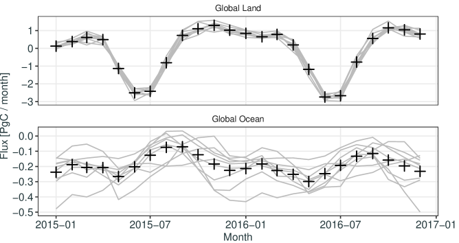
We now consider the case that is our main focus, where little to no direct verification data are available. An example of this, described in detail in Section 5, is the estimation of surface sources and sinks (fluxes) of CO2 in a MIP; see Figure 1, which shows the nine teams’ estimates of global land and global ocean non-fossil-fuel fluxes, as well as the unweighted ensemble average. Fluxes of CO2 occur over large temporal and geographical scales and are difficult to measure directly. One way their distribution is inferred indirectly is through their consequences on atmospheric concentrations of CO2, for which observations are available (Ciais et al.,, 2010). However, there are complications in using such indirect data taken anywhere in the atmosphere for verification, because issues such as overfitting and model misspecification mean that an accurate reproduction of the observed concentrations may not imply accurate fluxes (e.g., Houweling et al.,, 2010). Therefore, in this case and in cases like it, one is not applying REA’s criterion (ii), of agreement with flux data. However, according to REA criterion (i), one can infer the consensus between the MIP’s outputs (while taking into consideration model dependence, if needed). To apply the first criterion, we present a framework that enables statistically unbiased prediction and estimation (SUPE) based on an analysis of variance (ANOVA) statistical model, originally used for analyzing agricultural field experiments (Fisher,, 1935; Snedecor,, 1937). The framework promotes models that are in agreement and discounts those that are in disagreement, but it does so selectively in regions and seasons thought to have their own geophysical characteristics. For each of these regions/seasons, it provides a consensus summary and accompanying uncertainty quantification. It can also cater for model interdependencies when generating the summary, provided these have been, or can be, identified from a priori or expert knowledge.
Section 2 presents the ANOVA model in general, by recognizing that different factor combinations (e.g., spatial regions, seasons, geophysical-model configurations) will lead to agreement in differing degrees. We model the teams’ outputs for each factor combination as having different variances and, in Section 3, obtain statistically optimal weights based on these variances that allow optimal SUPE and its uncertainty quantification. In Section 4, we show how to estimate these weights using likelihood methods derived from the statistical distributions in the ANOVA model. Section 5 gives an illustration of our statistical-weighting methodology on the MIP published by Crowell et al., (2019), where nine teams produced outputs of global carbon-dioxide fluxes that were compared and summarized. A discussion of our framework, which we call SUPE-ANOVA, and conclusions, are given in Section 6.
2 Analysis of variance (ANOVA) for a MIP analysis
The area of statistics known as Experimental Design was born out of a need to control variations in agricultural field experiments, in order to compare and then select crop treatments based on replicate observations. The statistical ANOVA model was devised to analyze these experiments, and much has been written about it, starting with Fisher, (1935), Snedecor, (1937), Snedecor and Cochran in its eight editions (1957, …, 2014), and many other texts. It has been adopted in a number of disciplines driven by experimentation, including industrial manufacturing (e.g., Wu and Hamada,, 2000), and computer experiments where the so-called treatments are complex algorithms and code (e.g., Santner et al.,, 2010). We propose using the ANOVA framework for the analysis of outputs from important geophysical experiments performed within a MIP. It enables the output from many to be weighted in a statistically efficient manner to obtain one consensus estimate and a quantification of its uncertainty.
Let ‘’ represent a combination of factors (e.g., season, region) that the underlying geophysical process is expected to depend on, and let ‘’ index the output of the various teams participating in the MIP. By stratifying on each factor combination, we can write the output for the th factor combination () and the th team () as
| (1) |
where represents the number of replicates for factor combination . Each combination corresponds to a particular region/time-period in the MIP, and note that may differ for different factor combinations, reflecting the ability to capture complex MIP designs. In the analysis of the CO2-flux MIP given in Section 5, is a constant number (equal to six) for all regions and seasons.
The notation recognizes that each output is split into blocks (factor combinations) and, within the th block, there are outputs that are observing the same part of the geophysical process, corresponding to the replicates and the teams participating in the MIP. For example, suppose the MIP’s goal is to compare climate models’ projections of North American mean temperature between the years and , inclusive, at yearly intervals. Say the factor corresponds to decade, so . Further, corresponds to the years within a decade, and corresponds to the climate models. For climate model 17 (say) and decade 4 (say, which corresponds to the years between to , inclusive), the output at yearly intervals within the decade is .
The statistical ANOVA model proposed for (1) is, for , , and ,
| (2) |
where each have mean zero, , and . Here, is the MIP’s consensus of the geophysical process that each of the MIP outputs is attempting to estimate, and is the deviation from the consensus of the th output, assumed to have team-specific variances and covariances and to be independent of . Marginally, , where denotes a generic distribution with mean and variance . Dependence between teams’ outputs is captured with correlations . The statistical ANOVA model has variances that may differ from team to team. A mathematical-statistical result called the Gauss–Markov theorem (e.g., Casella and Berger,, 2006) implies that the hereto-referred weights are inversely proportional to these variances, and there is a more general version of the theorem that includes the dependencies between outputs; see Appendix B.
For and , we write the consensus as,
| (3) |
where each have mean zero. Here, is the unknown mean of the replicates, which we refer to as the climatological mean, and are random effects that capture variability in the replicates, and whose distribution we denote as . In the illustrative example of North American temperatures, indexes decade, corresponds to the consensus temperature in the th decade, while is the deviation from for the th year within the decade. The variability of temperatures can differ between decades, reflected by for . A temporal trend within the th decade could also be included in the model for . The team-specific variances and correlations defined through (2) may also be different for different decades. In the North American temperature example, a team’s output with higher weight in one decade may not have higher weight in another.
The statistical ANOVA model in (2) and (3) allows statistically unbiased prediction and estimation (SUPE) on the consensus for the climatological means, , and on the consensus for the underlying geophysical process, . Notice the heterogeneity of variation in (2) and (3), where the variances (and correlations) depend on both and . In the next section, we explain how knowledge of these variance (and correlation) parameters leads to statistically optimal weighting of the MIP outputs (1) for each when making inference on and .
3 Weighting MIP outputs for optimal inference
In the simple example from Section 2, of combining 20 climate models, not all models are expected to show the same variability. Different assumptions are made, say, about the model’s base resolution at which energy and water exchange takes place, how nonlinear dynamics are approximated, and so forth. This possibility is taken into account through (2), where the outputs from each team receives a different variance. A consequence of this is that, for optimal estimation and prediction of the consensus, different weights should be assigned to the different teams. This section discusses how to construct the optimal weights.
To illustrate optimal weighting in a simpler setting, without factor combinations, consider each climate model’s 2070 projected North American mean temperature (Tmp), . In this case, there is only one replication, so we omit the subscript on all quantities. To start with, assume a naïve statistical model wherein the 20 climate models all have the same variability:
| (4) |
where independently, . For simplicity of exposition, the correlations in this example are assumed to be zero. From (4), for . Then the best linear unbiased estimator (BLUE) of is the unweighted mean, and its variance is straightforward to calculate. That is,
| (5) |
To justify using the word ‘best’ in the acronym ‘BLUE,’ one needs to build a statistical model. Assuming the model (4), the estimate (5) is the most precise linear estimator, in that , for any other linear unbiased estimator, , of . However, (4) does not allow for different variabilities in the different MIP outputs.
Now, for the sake of argument, suppose that the first 15 out of the 20 climate models have an underlying resolution of , while the remaining five models have a resolution of . Consequently, an assumption of equal variance in the statistical distributions in (4) will need modification. Assume variances and are known, and
| (6) |
In Section 4, we show how these variances can be estimated. The parameter is still the target of inference but, under the statistical model (6), the Gauss–Markov theorem (e.g., Casella and Berger,, 2006) can be used to establish that the estimate in (5) is no longer the BLUE. We define the weights for estimating the projected mean temperature in the year 2070, , as follows:
| (7) |
Under the statistical model (6), the Gauss–Markov theorem can be used to establish that the BLUE (the most precise linear unbiased estimator) and its variance are, respectively,
| (8) |
That is, the statistically optimal weights for estimation of are given by (7), and the best estimator of is obtained by weighting each datum inversely proportional to its variance.
A more general statistical model, analogous to what we consider in (3), involves the random effect, , as follows:
| (9) |
where , and is assumed known. When , we recover the model (6), however the random effect plays an important role in recognizing the stochasticity in the projected temperature. Hence, for ,
| (10) |
Notice that there are between-model correlation terms induced by the random effect; for ,
where recall that in this simple example and are uncorrelated. Prediction of , which is the appropriate inference in the presence of the random effect, is made through the predictive distribution of given all the data from all the climate-model outputs; the optimal predictor of is the mean of this predictive distribution. We use the best linear unbiased predictor (BLUP) to make inference on . In the simple example of North American temperatures, the BLUP is
| (11) |
where
| (12) |
Notice that, for both optimal prediction (BLUP) and optimal estimation (BLUE), outputs with larger variability around the consensus receive lower weights. Additionally, for the BLUP given by (11), the weight on depends on how variable the underlying process is; that is, it depends on . Thus, the more variable the geophysical process is (captured through the parameter ), the less weight its mean receives in the optimal predictor, , of .
To justify the word ‘best’ in the acronym ‘BLUP,’ an uncertainty measure called the mean-squared prediction error (MSPE) is used. Let be any linear predictor of ; then the BLUP, , minimizes the MSPE since
A general formula for the MSPE of the BLUP is given later in this section.
Returning to the generic MIP, the steps to carry out optimally weighted linear inference follow the same line of development as in the temperature example: (1) specify the first-moment and second-moment parameters in the ANOVA model; (2) derive the variances and covariances of all random quantities in terms of the parameters; (3) weight the outputs (essentially) inversely proportional to their variances to obtain a BLUE/BLUP (i.e., to obtain a best SUPE); (4) quantify uncertainty (variance of the BLUE and MSPE of the BLUP). These four steps require an initialization that might be called a zeroth step, namely the estimation of the parameters and ; see Section 4. The correlation parameters, , could be known a priori or estimated using a likelihood-based methodology along with the variance parameters; see Appendix B. All together, these steps make up an inference framework for MIPs that we call SUPE-ANOVA.
We now give the optimal estimation and prediction formulas for the generic statistical ANOVA model under the assumption that the correlations between the models, , are zero; the general case of non-zero correlations involves matrix algebra and is given in Appendix B. From (2) and (3), it is straightforward to show that , , and . From a multivariate version of the Gauss-Markov theorem (e.g., Rencher and Christensen,, 2012), the BLUE of , and its variance, are given by
| (13) | ||||
| (14) |
for , where the optimal weights are
| (15) |
One-sigma and two-sigma confidence intervals for the unknown consensus mean , are given by and , respectively.
From (3), we also want to make inference on . Recall that , where are random quantities that capture the departures from the longer-term climatology given by , and they are assumed to have distribution . Since the goal of the MIP is to infer a consensus for the underlying process , BLUPs of these quantities are sought, along with their MSPEs. Straightforward use of the general Gauss–Markov Theorem (e.g., Rencher and Christensen,, 2012) results in the BLUP and its MSPE, as follows:
| (16) | ||||
| (17) |
where (for the moment) all parameters, including , are assumed known, and
| (18) |
One-sigma and two-sigma prediction intervals for are given by and , respectively.
In the next section, we give likelihood-based estimates of the model parameters, which we notate as , , and . Then the empirical BLUE/BLUP (written as EBLUE/EBLUP) equations are just those in (13)–(18) with the model parameters, , , and , replaced by their estimated quantities. This yields the EBLUE for , which we denote by , and an estimated variance denoted by . Further, it yields an EBLUP for , which we denote by , and an estimated mean-squared prediction error, denoted by . These formulas complete the specification of SUPE-ANOVA.
The likelihood-based estimates given in the next section require specification of statistical distributions and, to do this, we assume is for all distributions. When we assume Gaussianity, it should be noted that (16) is best among all possible predictors, not just linear ones (e.g., Cressie and Wikle,, 2011, Sec. 4.1.2).
4 The initialization step: Estimation of parameters
Estimation of the parameters of the ANOVA model given by (2) and (3) is performed under the assumption that all unknown distributions are Gaussian, which yields a likelihood function of the model’s parameters. The correlation parameters can be modeled and estimated, but they are assumed to be zero in the application in Section 5; here we omit them from the estimation equations, but see Appendix B where they are included. For the remaining parameters, it is known that the maximum likelihood estimates of variance parameters are biased and, to avoid this, we use restricted maximum likelihood (REML) estimation (Patterson and Thompson,, 1971; Harville,, 1977). REML estimation maximizes the restricted likelihood, denoted by , where is the -dimensional vector of all outputs from the MIP, is an -dimensional vector, and is an -dimensional vector. The definition of the restricted likelihood and a derivation of its analytical expression are given in Appendix B.
Small sample sizes can lead to variance estimates that need to be regularized in a manner similar to Twomey-Tikhonov regularization. This is achieved through the penalized restricted likelihood:
| (19) |
for
where and for fixed . The function is proportional to the density of an inverse gamma distribution with shape and scale , which is a common choice when making Bayesian inference on variance parameters. The value of the scales in the penalty is considered unknown and is estimated, whereas the shape is fixed and pre-specified to guard against one team’s output being over-weighted in the BLUEs/BLUPs. That is, for a given factor , the penalty puts a soft limit on the ratio between the largest and the smallest team-specific variances, , to a degree specified by , while the actual scale of the variances as a whole is left unknown and estimated through .
Calibration of the shape can be achieved by interpreting the penalty as a Bayesian prior on the variances. In that case, we specify that the ratio of the prior 97.5th percentile of the variances to the prior 2.5th percentile of the variances is equal to four, which yields the fixed value of . This choice means that it is unlikely that the largest variance is more than four times larger than the smallest variance.
The expression in (19) is maximized with respect to the model parameters and and with respect to the penalization scale , to yield the penalized REML estimates and . Appendix B gives the formulas for the general case where correlations are present. For , these estimates are substituted into (13), the BLUE for , to give the EBLUE of , denoted by , with empirical variance . For , , the EBLUP of , denoted by , with empirical MSPE, denoted by , is obtained similarly.
5 The OCO-2 MIP: Consensus CO2 fluxes
The rise in the atmospheric concentration of the greenhouse gas carbon dioxide (CO2) is the main determinant of global warming (IPCC,, 2013), and estimation of the sources and sinks (called fluxes) of CO2 is a high priority for the global community (Friedlingstein et al.,, 2014). Fluxes of CO2 arise from both anthropogenic and natural processes, and the latter are hard to observe directly, as they occur over large spatial and temporal scales. One way to estimate the natural fluxes, called flux inversion, is through observation of their influence on atmospheric concentrations of CO2. As natural fluxes are so difficult to measure otherwise, flux inversions for CO2 play an important role in quantifying Earth’s carbon budget.
Flux inversion is an ill-posed inverse problem, in which an atmospheric transport model is used to simulate the transport of the trace gas from its sources to the times and places of its observation. The transport model is combined with a procedure, usually based on a Bayesian state-space model, to work backwards from observations to fluxes. The data used by inversions are typically a combination of surface, aircraft, and ship observations, and data collected by spaceborne instruments. In this section, we shall use the output from a MIP based on CO2 data from NASA’s Orbiting Carbon Observatory-2 (OCO-2) satellite (Crowell et al.,, 2019) to obtain consensus flux estimates and predictions.
Flux inversion is subject to many forms of model uncertainty, which complicate interpretation of the estimated fluxes. These uncertainties stem from questions about the fidelity of simulated atmospheric transport, about how best to parameterize the unknown fluxes, and about the choice of prior for the flux field, among others. To address these in a rigorous manner, the OCO-2 project established a series of MIPs where an ensemble of flux outputs was assembled from submissions by different teams, who performed global flux inversions under a common protocol. The MIPs involve the use of OCO-2 retrievals of the vertical column–average CO2 concentration, as well as flask and in situ observations of CO2 concentrations.
The first of the MIPs concluded in 2019, and its results were reported by Crowell et al., (2019). The satellite data in this MIP were based on version 7r of the OCO-2 data, so henceforth we refer to it as MIPv7. Nine teams participated in MIPv7. The results were released as a set of aggregated monthly non-fossil-fuel fluxes spanning 27 disjoint, large regions derived from TransCom3 regions, shown in Figure A1 (where the unlabeled areas are assumed to have zero flux) and listed in Table A1. The outputs from the MIP covered each month over the two years from January 2015 to December 2016, inclusive. Each team was tasked with producing estimated fluxes from three observation types: from an inversion based on flask and in situ measurements only (IS), from an inversion based on OCO-2 retrievals made in land glint (LG) mode, and from an inversion based on OCO-2 retrievals made in land nadir (LN) mode.
To apply the SUPE-ANOVA framework to MIPv7, the fluxes from each mode were considered separately. Then, the factor of interest is , where is a season (starting with December-January-February [DJF]), and is a spatial region. The replicates are the six months within a season for the two-year study period, so for all factors. From (2) and (3), the flux output of the th team is modeled by,
| (20) |
for , where are uncorrelated; we assume they are uncorrelated for simplicity, but, if desired, it is relatively easy to incorporate correlations using the equations in Appendix B. The consensus flux is modeled by
| (21) |
The term represents the MIP consensus for the underlying geophysical flux for month in season and region ; is the more-slowly-varying consensus climatological flux for the season and region; is the variance of the deviations of the monthly fluxes from the climatological flux; and is the variance of the th team’s flux output within each region and season.
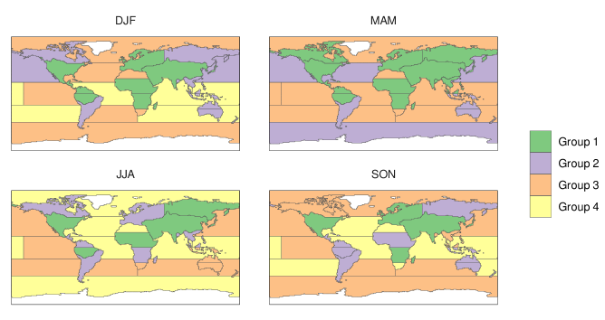
The six replicates within each factor are too few for reliable estimation of the variance parameters, but this can be addressed straightforwardly by grouping regions with similar variability within a season. Hence, for the four seasons , variance parameters , , and the penalization scales were constrained to have identical values within grouped regions. We present a clustering approach to construct groups in Appendix C; the chosen groups are shown in Figure A2.
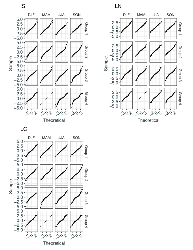
The parameters of the model in (20) and (21) were estimated according to the initialization step given in Section 4, and the SUPE-ANOVA framework was used to obtain the consensus flux predictions . To check whether the model has good fit to the fluxes, we define the standardized errors, , for , , , and . Under the Gaussian assumptions used to fit the model, the standardized errors should be approximately . We diagnosed this visually using Q-Q plots, by plotting for each season and group of regions against the theoretical quantiles of the distribution; under the assumptions, the relationship should be approximately on a 45 line. Figure A3 shows these Q-Q plots, which do not indicate any obvious violations of the model assumptions.
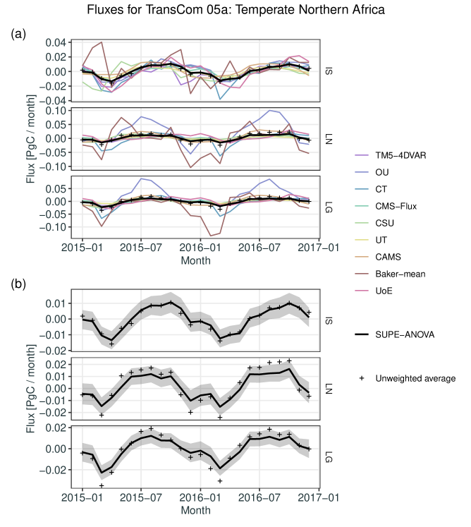
As an example of predicting consensus fluxes at the regional level, Figure 2(a) shows the SUPE-ANOVA predictions as a time series for one region, T05a (Temperate Northern Africa), as well as the time series of fluxes from each of the nine MIP participants; the unweighted averages, , are also shown. Separate panels give the time series for each observation type (IS, LN, and LG). Figure 2(b) repeats Figure 2(a) but with the participating teams’ fluxes omitted to allow the vertical axis to be re-scaled. It also shows 95% prediction intervals for the predicted consensus fluxes, where the upper and lower values are . For the IS fluxes in the region T05a, the predicted consensus hardly differs from the unweighted average. By contrast, for the LN and LG fluxes, the predicted consensus sometimes differs significantly from the unweighted average.
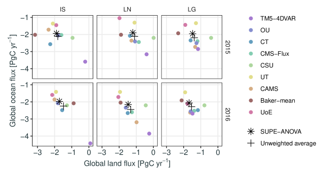
The SUPE-ANOVA predictions of the consensus fluxes and the unweighted-average fluxes at the regional level were also aggregated spatially and temporally to yield the annual global land and annual global ocean fluxes. These are shown in Figure 3, which also shows the land–ocean aggregates for the nine teams in the MIP. Fluxes are given for all three observation types, IS, LN, and LG, and for both study years, 2015 and 2016. The SUPE-ANOVA consensus fluxes imply a larger land sink and a smaller ocean sink than do the unweighted averages. Also, for the IS observation type, there are more extreme values from the TM5-4DVAR team then the other teams, and these have been downweighted in the consensus estimate, relative to the weights they received in the unweighted average.
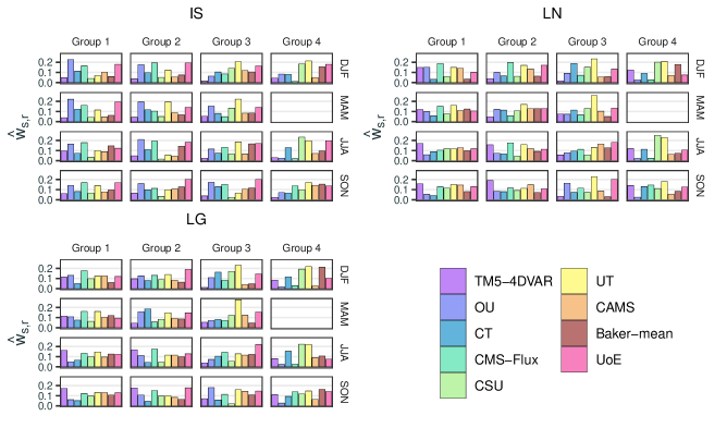
The different teams’ weights used in the SUPE-ANOVA framework vary between seasons and regions, although they are identical within the cluster groups. For a given , define the climatological weights, , for . From (13), these weights correspond to the relative weighting of each participant in estimating the consensus mean climatological flux, . Figure 4 shows the climatological weights for the three observation types (IS, LN, LG), for each season and grouping of regions within each season. From inspection of the weights in Figure 4, the UT team and the UoE team generally have higher weights due to their associated estimated variances being consistently smaller.
6 Discussion and conclusions
A reader of this article might ask whether in the North American temperature example given in Section 3, the simple unweighted average of the MIP outputs provides a reasonable estimate of . Under the SUPE-ANOVA framework, that estimate given by Equation (5) is unbiased. However, it is not a statistically efficient estimator under our consensus model. This can have a profound effect on the design of the MIP. Using the optimal weights, namely, inversely proportional to for , means that the precision of can be matched to the precision of but with (much) less than 20. Since is also unbiased, this optimally weighted mean has a distinct inferential advantage over the unweighted mean, , when both are based on the same outputs . Furthermore, the simple variance, , in Equation (5) is an incorrect expression for when it is no longer true that . The correct expression is
which will give valid consensus inferences and correct coverage for the one-sigma and two-sigma intervals presented in Section 3, albeit wider than the intervals based on .
A number of articles reviewed in Section 1 have taken a Bayesian viewpoint (Tebaldi et al.,, 2005; Manning et al.,, 2009; Smith et al.,, 2009; Tebaldi and Sansó,, 2009; Chandler,, 2013). A Bayesian spatial ANOVA was used in Sain et al., (2011), Kang et al., (2012), and Kang and Cressie, (2013) to analyze projected temperature in a MIP called the North American Regional Climate Change Assessment Program (NARCCAP; see Mearns et al.,, 2012). This approach adds another layer of complexity to consensus inference in a MIP, where prior distributions on mean and variance parameters need to be specified, sensitivity to the specification assessed, and posterior-distribution sampling algorithms developed. In contrast, our SUPE-ANOVA framework does not depend on priors, is fast to compute, and results in easy-to-interpret weights on the MIP outputs within the ANOVA factors (e.g., season, region).
We return to the general SUPE-ANOVA framework developed in Sections 2 and 3 to show how the optimal weights could be used in conjunction with verification data. Let denote the verification data, with associated measurement-error variances . Each datum can be indexed according to which factor and replicate it belongs. Hence, rewrite as , which will be compared to the outputs, . Then a simple and statistically justifiable way to assign weights to each team’s output is to define
| (22) |
where . Equation (22) shows how the SUPE-ANOVA weights, , can be used to define a prior in a Bayesian Model Averaging (BMA) scheme, where can be interpreted as the posterior weights assigned to the models, given the verification data . That is, the models are weighted based on verification data without making the common ‘truth-plus-error’ assumption (Bishop and Abramowitz,, 2013), or even without making the more general assumption of co-exchangeability between the MIP outputs and the data (Rougier et al.,, 2013). Now, since the BMA weights have lost their dependence on the factors, they will not yield optimal estimates of , or optimal predictions of ; instead, they can be used to suggest which model is the most reliable overall in the sense of REA.
In summary, basic statistical principles have been followed to make optimal consensus inference in a MIP. Once the variance/covariance parameters in the SUPE-ANOVA framework have been estimated in an initialization step, the weights are immediate; code in the R programming language (R Core Team,, 2020) is available at https://github.com/mbertolacci/supe-anova-paper for the OCO-2 MIP analyzed in Section 5.
Acknowledgements
This project was largely supported by the Australian Research Council (ARC) Discovery Project (DP) DP190100180 and NASA ROSES grant NNH20ZDA001N-OCOST. Noel Cressie’s research was also supported by ARC DP150104576, and Andrew Zammit-Mangion’s research was also supported by an ARC Discovery Early Career Research Award (DECRA) DE180100203. The authors are grateful to the OCO-2 Flux Group for their feedback and suggestions.
Data Availability Statement
The data for the OCO-2 MIP analyzed in Section 5 are described by Crowell et al., (2019) and may be found on the OCO-2 MIPv7 website hosted by the NOAA Global Monitoring Laboratory (https://gml.noaa.gov/ccgg/OCO2/).
References
- Abramowitz et al., (2019) Abramowitz, G., et al. (2019). ESD Reviews: Model dependence in multi-model climate ensembles: Weighting, sub-selection and out-of-sample testing. Earth System Dynamics, 10(1), 91–105, https://doi.org/10.5194/esd-10-91-2019.
- Bishop and Abramowitz, (2013) Bishop, C. H. & Abramowitz, G. (2013). Climate model dependence and the replicate Earth paradigm. Climate Dynamics, 41(3), 885–900, https://doi.org/10.1007/s00382-012-1610-y.
- Boé, (2018) Boé, J. (2018). Interdependency in Multimodel Climate Projections: Component Replication and Result Similarity. Geophysical Research Letters, 45(6), 2771–2779, https://doi.org/10.1002/2017GL076829.
- Casella and Berger, (2006) Casella, G. & Berger, R. L. (2006). Statistical Inference, second edition. Pacific Grove, CA: Duxbury Press.
- Chandler, (2013) Chandler, R. E. (2013). Exploiting strength, discounting weakness: Combining information from multiple climate simulators. Philosophical Transactions of the Royal Society A: Mathematical, Physical and Engineering Sciences, 371(1991), 20120388, https://doi.org/10.1098/rsta.2012.0388.
- Ciais et al., (2010) Ciais, P., Rayner, P., Chevallier, F., Bousquet, P., Logan, M., Peylin, P., & Ramonet, M. (2010). Atmospheric inversions for estimating CO2 fluxes: Methods and perspectives. Climatic Change, 103(1), 69–92, https://doi.org/10.1007/s10584-010-9909-3.
- Cressie and Wikle, (2011) Cressie, N. & Wikle, C. K. (2011). Statistics for Spatio-Temporal Data. Hoboken, NJ: Wiley.
- Crowell et al., (2019) Crowell, S., et al. (2019). The 2015–2016 carbon cycle as seen from OCO-2 and the global in situ network. Atmospheric Chemistry and Physics, 19, 9797–9831, https://doi.org/10.5194/acp-19-9797-2019.
- Fisher, (1935) Fisher, R. A. (1935). The Design of Experiments. Edinburgh, UK: Oliver and Boyd.
- Flato et al., (2014) Flato, G., et al. (2014). Evaluation of climate models. In T. Stocker, D. Qin, G.-K. Plattner, M. Tignor, S. K. Allen, J. Boschung, A. Nauels, Y. Xia, V. Bex, & P. M. Midgley (Eds.), Climate Change 2013: The Physical Science Basis. Contribution of Working Group I to the Fifth Assessment Report of the Intergovernmental Panel on Climate Change (pp. 741–866). Cambridge University Press, Cambridge UK and New York, NY.
- Friedlingstein et al., (2014) Friedlingstein, P., Meinshausen, M., Arora, V. K., Jones, C. D., Anav, A., Liddicoat, S. K., & Knutti, R. (2014). Uncertainties in CMIP5 climate projections due to carbon cycle feedbacks. Journal of Climate, 27, 511–526, https://doi.org/10.1175/JCLI-D-12-00579.1.
- Giorgi and Mearns, (2002) Giorgi, F. & Mearns, L. O. (2002). Calculation of average, uncertainty range, and reliability of regional climate changes from AOGCM simulations via the “reliability ensemble averaging” (REA) method. Journal of Climate, 15(10), 1141–1158, https://doi.org/10.1175/1520-0442(2002)015<1141:COAURA>2.0.CO;2.
- Harville, (1977) Harville, D. A. (1977). Maximum likelihood approaches to variance component estimation and to related problems. Journal of the American Statistical Association, 72, 320–338, https://doi.org/10.1080/01621459.1977.10480998.
- Haughton et al., (2015) Haughton, N., Abramowitz, G., Pitman, A., & Phipps, S. J. (2015). Weighting climate model ensembles for mean and variance estimates. Climate Dynamics, 45(11), 3169–3181, https://doi.org/10.1007/s00382-015-2531-3.
- Houweling et al., (2010) Houweling, S., et al. (2010). The importance of transport model uncertainties for the estimation of CO2 sources and sinks using satellite measurements. Atmospheric Chemistry and Physics, 10(20), 9981–9992, https://doi.org/10.5194/acp-10-9981-2010.
- IPCC, (2013) IPCC (2013). Climate Change 2013: The Physical Science Basis. Working Group I Contribution to the Fifth Assessment Report of the Intergovernmental Panel on Climate Change. Cambridge, United Kingdom and New York, NY, USA: Cambridge University Press.
- Kang and Cressie, (2013) Kang, E. L. & Cressie, N. (2013). Bayesian hierarchical ANOVA of regional climate-change projections from NARCCAP Phase II. International Journal of Applied Earth Observation and Geoinformation, 22, 3–15, https://doi.org/10.1016/j.jag.2011.12.007.
- Kang et al., (2012) Kang, E. L., Cressie, N., & Sain, S. R. (2012). Combining outputs from the North American Regional Climate Change Assessment Program by using a Bayesian hierarchical model. Journal of the Royal Statistical Society: Series C (Applied Statistics), 61(2), 291–313, https://doi.org/10.1111/j.1467-9876.2011.01010.x.
- Kirtman et al., (2013) Kirtman, B., et al. (2013). Near-term climate change: Projections and predictability. In T. Stocker, D. Qin, G.-K. Plattner, M. Tignor, S. Allen, J. Boschung, A. Nauels, Y. Xia, V. Bex, & P. Midgley (Eds.), Climate Change 2013: The Physical Science Basis. Contribution of Working Group I to the Fifth Assessment Report of the Intergovernmental Panel on Climate Change (pp. 953–1028). Cambridge, United Kingdom and New York, NY, USA: Cambridge University Press.
- Knutti, (2010) Knutti, R. (2010). The end of model democracy? Climatic Change, 102, 395–404, https://doi.org/10.1007/s10584-010-9800-2.
- Knutti et al., (2010) Knutti, R., Furrer, R., Tebaldi, C., Cermak, J., & Meehl, G. A. (2010). Challenges in combining projections from multiple climate models. Journal of Climate, 23(10), 2739–2758, https://doi.org/10.1175/2009JCLI3361.1.
- Knutti et al., (2013) Knutti, R., Masson, D., & Gettelman, A. (2013). Climate model genealogy: Generation CMIP5 and how we got there. Geophysical Research Letters, 40(6), 1194–1199, https://doi.org/10.1002/grl.50256.
- Knutti et al., (2017) Knutti, R., Sedláček, J., Sanderson, B. M., Lorenz, R., Fischer, E. M., & Eyring, V. (2017). A climate model projection weighting scheme accounting for performance and interdependence. Geophysical Research Letters, 44(4), 1909–1918, https://doi.org/10.1002/2016GL072012.
- Krishnamurti et al., (2000) Krishnamurti, T. N., et al. (2000). Multimodel ensemble forecasts for weather and seasonal climate. Journal of Climate, 13(23), 4196–4216, https://doi.org/10.1175/1520-0442(2000)013<4196:MEFFWA>2.0.CO;2.
- Manning et al., (2009) Manning, L. J., Hall, J. W., Fowler, H. J., Kilsby, C. G., & Tebaldi, C. (2009). Using probabilistic climate change information from a multimodel ensemble for water resources assessment. Water Resources Research, 45(11), https://doi.org/10.1029/2007WR006674.
- Mearns et al., (2012) Mearns, L. O., et al. (2012). The North American Regional Climate Change Assessment Program: Overview of phase I results. Bulletin of the American Meteorological Society, 93(9), 1337–1362, https://doi.org/10.1175/BAMS-D-11-00223.1.
- Meehl et al., (2000) Meehl, G. A., Boer, G. J., Covey, C., Latif, M., & Stouffer, R. J. (2000). The Coupled Model Intercomparison Project (CMIP). Bulletin of the American Meteorological Society, 81(2), 313–318, https://doi.org/10.1175/1520-0477(2000)080<0305:MROTEA>2.3.CO;2.
- Patterson and Thompson, (1971) Patterson, H. D. & Thompson, R. (1971). Recovery of inter-block information when block sizes are unequal. Biometrika, 58, 545–554, https://doi.org/10.1093/biomet/58.3.545.
- R Core Team, (2020) R Core Team (2020). R: A Language and Environment for Statistical Computing. R Foundation for Statistical Computing, Vienna, Austria. https://www.R-project.org/.
- Reifen and Toumi, (2009) Reifen, C. & Toumi, R. (2009). Climate projections: Past performance no guarantee of future skill? Geophysical Research Letters, 36(13), https://doi.org/10.1029/2009GL038082.
- Rencher and Christensen, (2012) Rencher, A. C. & Christensen, W. F. (2012). Methods of Multivariate Analysis, third edition. Hoboken, NJ: Wiley.
- Rougier et al., (2013) Rougier, J., Goldstein, M., & House, L. (2013). Second-order exchangeability analysis for multimodel ensembles. Journal of the American Statistical Association, 108(503), 852–863, https://doi.org/10.1080/01621459.2013.802963.
- Sain et al., (2011) Sain, S. R., Nychka, D., & Mearns, L. (2011). Functional ANOVA and regional climate experiments: A statistical analysis of dynamic downscaling. Environmetrics, 22(6), 700–711, https://doi.org/10.1002/env.1068.
- Sanderson et al., (2017) Sanderson, B. M., Wehner, M., & Knutti, R. (2017). Skill and independence weighting for multi-model assessments. Geoscientific Model Development, 10(6), 2379–2395, https://doi.org/10.5194/gmd-10-2379-2017.
- Santner et al., (2010) Santner, T. J., Williams, B. J., & Notz, W. I. (2010). The Design and Analysis of Computer Experiments. New York, NY: Springer.
- Shepherd et al., (2018) Shepherd, A., et al. (2018). Mass balance of the Antarctic Ice Sheet from 1992 to 2017. Nature, 558(7709), 219–222, https://doi.org/10.1038/s41586-018-0179-y.
- Smith et al., (2009) Smith, R. L., Tebaldi, C., Nychka, D., & Mearns, L. O. (2009). Bayesian modeling of uncertainty in ensembles of climate models. Journal of the American Statistical Association, 104(485), 97–116, https://doi.org/10.1198/jasa.2009.0007.
- Snedecor, (1937) Snedecor, G. W. (1937). Statistical Methods Applied to Experiments in Agriculture and Biology, first edition. Ames, IA: Collegiate Press.
- Snedecor and Cochran, (2014) Snedecor, G. W. & Cochran, W. G. (2014). Statistical Methods, eighth edition. Chichester, UK: Wiley.
- Sunyer et al., (2014) Sunyer, M. A., Madsen, H., Rosbjerg, D., & Arnbjerg-Nielsen, K. (2014). A Bayesian approach for uncertainty quantification of extreme precipitation projections including climate model interdependency and nonstationary bias. Journal of Climate, 27(18), 7113–7132, https://doi.org/10.1175/JCLI-D-13-00589.1.
- Tebaldi and Knutti, (2007) Tebaldi, C. & Knutti, R. (2007). The use of the multi-model ensemble in probabilistic climate projections. Philosophical Transactions of the Royal Society A: Mathematical, Physical and Engineering Sciences, 365(1857), 2053–2075, https://doi.org/10.1098/rsta.2007.2076.
- Tebaldi and Sansó, (2009) Tebaldi, C. & Sansó, B. (2009). Joint projections of temperature and precipitation change from multiple climate models: A hierarchical Bayesian approach. Journal of the Royal Statistical Society: Series A (Statistics in Society), 172(1), 83–106, https://doi.org/10.1111/j.1467-985X.2008.00545.x.
- Tebaldi et al., (2005) Tebaldi, C., Smith, R. L., Nychka, D., & Mearns, L. O. (2005). Quantifying uncertainty in projections of regional climate change: A Bayesian approach to the analysis of multimodel ensembles. Journal of Climate, 18(10), 1524–1540, https://doi.org/10.1175/JCLI3363.1.
- Wu and Hamada, (2000) Wu, C. F. J. & Hamada, M. (2000). Experiments: Planning, Analysis, and Parameter Design Optimization. New York, NY: Wiley.
Appendices
Appendix A Additional Figures and Tables
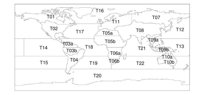
| Code | Name | Code | Name |
|---|---|---|---|
| T01 | North American Boreal | T10b | Temperate Australia |
| T02 | North American Temperate | T11 | Europe |
| T03a | Northern Tropical South America | T12 | North Pacific Temperate |
| T03b | Southern Tropical South America | T13 | West Pacific Tropical |
| T04 | South American Temperate | T14 | East Pacific Tropical |
| T05a | Temperate Northern Africa | T15 | South Pacific Temperate |
| T05b | Northern Tropical Africa | T16 | Northern Ocean |
| T06a | Southern Tropical Africa | T17 | North Atlantic Temperate |
| T06b | Temperate Southern Africa | T18 | Atlantic Tropical |
| T07 | Eurasia Boreal | T19 | South Atlantic Temperate |
| T08 | Eurasia Temperate | T20 | Southern Ocean |
| T09a | Northern Tropical Asia | T21 | Indian Tropical |
| T09b | Southern Tropical Asia | T22 | South Indian Temperate |
| T10a | Tropical Australia |
Appendix B The general SUPE-ANOVA equations and the restricted likelihood
To derive the general estimation/prediction equations and the restricted likelihood of the ANOVA model given by (2) and (3), we first rewrite the model in matrix-vector form as
| (23) |
where is a -dimensional vector; is an -dimensional vector; is a -dimensional vector; and and are matrices of ones and zeros that map the entries of and , respectively, to the appropriate entries of . Let and . The matrix is diagonal with the entries of on its diagonal, while has the entries of on its diagonal and in its off-diagonal entries. For both matrices, the entries are repeated as needed for each replicate . Under (23), the marginal mean and variance of are, therefore, and , respectively.
The multivariate Gauss–Markov theorem (e.g., Rencher and Christensen,, 2012) yields the BLUE under (23) as
| (24) |
The variance of is given by . The BLUP for is then
| (25) |
with prediction variance . The BLUP and prediction variance for follow as and , respectively. When for and , the vector expressions for the BLUE and the BLUP given here can be shown to be equivalent to the element-wise expressions (13) and (16), respectively.
To derive the restricted likelihood, we first assume that all unknown distributions are Gaussian. Under this assumption, the distribution of is multivariate normal with . Viewed as a function of its parameters, , , and , where and are defined in Section 4, the density of this distribution is the likelihood . The restricted likelihood is equal to the integral of the likelihood with respect to (Harville,, 1977); that is,
where the constant of proportionality does not depend on the unknown parameters. Where is assumed to be known, as in Sections 4 and 5, we write the restricted likelihood as .
Appendix C Clustering procedure to group regions of similar variability
For the OCO-2 MIPv7 example in Section 5, we established the groupings of regions with similar variability as follows: Let be the empirical median of the set , where is the empirical median of the set . The value is a robust empirical estimate of the ensemble variability in the season and region. We then divided the 27 regions into groups that are assumed to have identical variances by applying -means clustering to the set . The clustering is therefore based on the order of magnitude of the ensemble variability. The number of clusters, , was chosen as the smallest such that the sum of the within-cluster sums-of-squares is at least 90% of the total sums-of-squares. The fluxes derived from the LN observation type were used to do the clustering, and the same clusters were then used on the fluxes derived from the LG and the IS observation types. The resulting groupings of regions are shown in Figure A2; the group numbers are ordered from the clustered regions exhibiting the most variability (Group 1 has the highest average ) to those exhibiting the least variability. Four clusters were chosen for DJF, JJA, and SON, and three clusters for MAM.