This paper was converted on www.awesomepapers.org from LaTeX by an anonymous user.
Want to know more? Visit the Converter page.

Full statistics of nonequilibrium heat and work for many-body quantum Otto engines and universal bounds: A nonequilibrium Green’s function approach

Sandipan Mohanta mohanta.sandipan@students.iiserpune.ac.in Department of Physics, Indian Institute of Science Education and Research, Pune 411008, India    Bijay Kumar Agarwalla bijay@iiserpune.ac.in Department of Physics, Indian Institute of Science Education and Research, Pune 411008, India bijay@iiserpune.ac.in
Abstract

We consider a generic four-stroke quantum Otto engine consisting of two unitary and two thermalization strokes with an arbitrary many-body working medium. Using the Schwinger-Keldysh nonequilibrium Green’s function formalism, we provide an analytical expression for the cumulant generating function corresponding to the joint probability distribution of nonequilibrium work and heat. The obtained result is valid up to the second order of the external driving amplitude. We then focus on the linear response limit and obtain Onsager’s transport coefficients for the generic Otto cycle and showed that the traditional fluctuation-dissipation relation for the total work is violated in the quantum domain, whereas for heat it is preserved. This leads to remarkable consequences in obtaining universal constraints on heat and work fluctuations for engine and refrigerator regimes of the Otto cycle and further allows us to make connections to the thermodynamic uncertainty relations. These findings are illustrated using a paradigmatic model that can be feasibly implemented in experiments.

I Introduction

Thermodynamic cycles are fundamental concepts in the field of thermodynamics that describe the exchange and conversion of energy and play a crucial role in understanding and optimizing the performance of various energy conversion devices Çengel and Boles (2004). Traditionally, thermodynamics provides a description of systems in terms of bulk or macroscopic properties by focusing primarily on averages or mean values of thermodynamic quantities Zemansky (1968); Callen et al. (1985). However, for small-scale systems consisting of a few degrees of freedom, thermal and quantum fluctuations about the mean values can be significant. Exploring the universal properties of these fluctuations for out-of-equilibrium systems has been of key interest in the field of stochastic and quantum thermodynamics Jarzynski (2011); Seifert (2012, 2008); Goold et al. (2016); Vinjanampathy and Anders (2016). Significant theoretical insight has been achieved in this regard over the past two decades, owing to the diverse kinds of universal fluctuation relations Jarzynski (2011); Holubec and Ryabov (2021); Esposito et al. (2009); Campisi et al. (2011).

In recent times, quantum engines have garnered significant interest as they provide a privileged platform to investigate the intricate relationship between quantum phenomena and nonequilibrium thermodynamics. Furthermore, they offer opportunities to harness the unique properties of the quantum working medium to boost performance and enhance stability Jaramillo et al. (2016); Vroylandt et al. (2018); Niedenzu and Kurizki (2018); Boubakour et al. (2023). Thanks to rapid technological developments, it has now become possible to fabricate small-scale thermal machines Peterson et al. (2019); Myers et al. (2022a); Blickle and Bechinger (2012); Martínez et al. (2016, 2017); Bouton et al. (2021); Maslennikov et al. (2019); Abah et al. (2012a); Roßnagel et al. (2016); Zhang et al. (2022); Bhattacharjee and Dutta (2021). For example, the smallest possible quantum Otto engine, with a qubit as working fluid has been realized in an NMR setup Peterson et al. (2019). Another paradigmatic model, a harmonic oscillator heat engine has also been realized in the ion-trap setup Roßnagel et al. (2016). More complex and exotic many-body working fluids executing a cycle has now been proposed Carollo et al. (2020); Chen et al. (2019); Sun et al. (2017); Altintas et al. (2014); Thomas and Johal (2011); Huang et al. (2013a); Myers et al. (2022b); Henrich et al. (2007a); Huang et al. (2013b); Singh and Rebari (2020); Jaramillo et al. (2016).

The study of fluctuation in the context of such small-scale thermal machines is of tremendous significance Watanabe and Minami (2022); Ito et al. (2019); Denzler and Lutz (2020); Pietzonka and Seifert (2018a); Jiao et al. (2021). Recently, there have been intense ongoing efforts to quantify the performance of quantum engines involving efficiency, power, and power fluctuation or so-called constancy Pietzonka and Seifert (2018b). In this regard, Thermodynamic uncertainty relations (TURs), establishing a trade-off relation between the relative fluctuation of thermodynamic currents and entropy production, have been put forward that rule out the possibility of achieving Carnot efficiency without allowing power fluctuation to diverge Barato and Seifert (2015); Pietzonka and Seifert (2018b); Gingrich et al. (2016); Falasco et al. (2020); Guarnieri et al. (2019); Brandner et al. (2018); Agarwalla and Segal (2018). Another direction of studies established universal upper and lower bounds on the ratio of power to input heat current fluctuations of generic continuously coupled autonomous thermal machines operating in the linear response regime Saryal et al. (2021). These studies have been further extended to discrete four-stroke Otto cycles with specific working mediums Saryal and Agarwalla (2021); Mohanta et al. (2023) and very recently for model-specific periodically driven continuous machines Das et al. (2023). However, a detailed understanding of the bounds on nonequilibrium fluctuations for non-autonomous machines with generic many-body working medium is still lacking.

In this work, we consider a generic four-stroke quantum Otto cycle Solfanelli et al. (2020); Kosloff (2019); Geva and Kosloff (1992); Feldmann and Kosloff (2000); Kieu (2004); Henrich et al. (2007b); Scully (2002); Watanabe et al. (2017); Rezek and Kosloff (2006); Lin and Chen (2003); Abah et al. (2012b); Kosloff and Rezek (2017); Uzdin et al. (2015) consisting of an arbitrary many-body working medium and derive an analytical expression for the joint cumulant generating function (CGF) of total work and input heat, valid up to the second order of the driving amplitude, by employing the rigorous Schwinger-Keldysh nonequilibrium Green’s function (NEGF) formalism Fei and Quan (2020); Cavina et al. (2023); Rammer and Smith (1986); Schwinger (1961). The CGF obtained for an arbitrary many-body working medium satisfies the nonequilibrium fluctuation relation Campisi (2014). Furthermore, we demonstrate the linear response limit characterized by a small driving amplitude and small temperature difference and obtain the expressions for the Onsager’s transport coefficients. Notably, we reveal a breakdown of the traditional fluctuation-dissipation relation (FDR) Kubo (1966); Weber (1956); Felderhof (1978); Pathria and Beale (2021) for the total work, while, the traditional FDR remains intact for heat. Our findings have remarkable implications for the generic Otto cycle: when operating as an engine, the ratio of output (work) to input (heat from the hot reservoir) fluctuations is universally bounded from below, while in the refrigerator regime, a similar quantity is universally bounded from above. Additionally, we also establish connections to the TURs. Finally, we compare the obtained universal bounds for the discrete Otto cycle with those of autonomous steady-state machines Saryal et al. (2021); Mohanta et al. (2023); Saryal and Agarwalla (2021); Das et al. (2023).

We organize the paper as follows: Section II briefly describes the quantum Otto cycle and the two-point measurement protocol to construct the CGF corresponding to the joint probability distribution of total work and heat. We then demonstrate how to map the CGF on the modified Keldysh contour. In Section III, we obtain the expression for the CGF valid up to the second order of the external driving amplitude. We validate that the CGF respects the fluctuation symmetry. In Section IV, we discuss the linear response limit, obtain the Onsager transport coefficients, and derive universal bounds on nonequilibrium fluctuations. We illustrate the obtained results with a paradigmatic model in Section V. Finally, we summarize our main findings and provide an outlook in Section VI.

II Quantum Otto cycle and Characteristic function on modified Schwinger-Keldysh contour

We consider a generic many-body working medium for the quantum Otto cycle and treat the many-body interaction part as a time-dependent perturbation. The total Hamiltonian of the working fluid is given by

H(t)=H0+λ(t)H1,H(t)=H_{0}+\lambda(t)H_{1}, (1)

where H0H_{0} is the non-interacting part, often referred to here as the free Hamiltonian, and H1H_{1} represents an arbitrary many-body interaction term. λ(t)\lambda(t) is an arbitrary driving protocol that drives the system away from equilibrium. Importantly, λ(t)\lambda(t) serves the purpose of a perturbation parameter, and the values it can take are significantly smaller than those of other dimensionally comparable free parameters.

Refer to caption
Figure 1: Schematic of a four-stroke Otto cycle with a many-body quantum working medium executing two unitary and two thermalization strokes. The expansion stroke is carried out by the unitary protocol 𝒰e{\cal U}_{\rm e} and the compression stroke is carried out by the 𝒰c=Θ𝒰eΘ{\cal U}_{\rm c}\!=\!\Theta\mathcal{U}_{\mathrm{e}}^{\dagger}\Theta^{\dagger}. The final states of the unitary strokes at BB and DD are non-thermal ones. The isochoric thermalization strokes take place in the presence of the reservoirs.

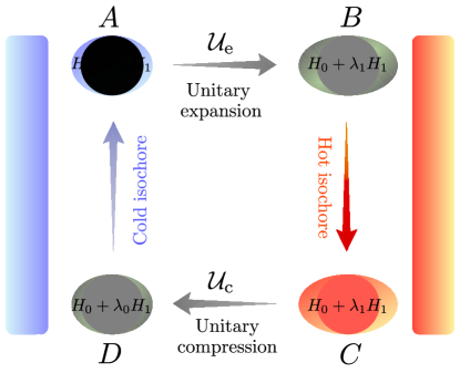
The working medium performs a four-stroke Otto cycle consisting of two unitary and two thermalization strokes with respect to the cold and hot thermal reservoirs with fixed inverse temperatures βc\beta_{c} and βh\beta_{h}, respectively (see Fig. 1). Below we briefly describe these four strokes: (1) Unitary expansion stroke (ABA\!\to\!B). The system starts at time t=0t\!=\!0 from the initial thermal state AA characterized by the cold inverse temperature βc\beta_{c} and Hamiltonian H(0)=H0+λ(0)H1H(0)\!=\!H_{0}+\lambda(0)H_{1}, where λ(0)=λ0\lambda(0)\!=\!\lambda_{0}. The system is then decoupled from the reservoir and λ(t)\lambda(t) drives the system out of equilibrium. The first unitary stroke ends at time t=τ1t\!=\!\tau_{1} with λ(τ1)=λ1\lambda(\tau_{1})\!=\!\lambda_{1}. At the end of this stroke, the state of the system BB is a non-thermal one. (2) Hot isochore (BCB\!\to\!C). During the first heat exchange stroke, the system is brought into weak contact with the hot reservoir while keeping λ1\lambda_{1} fixed. The system then waits until it reaches a thermal state CC, parameterized by (λ1,βh\lambda_{1},\beta_{h}) at time t=τ1+τht\!=\!\tau_{1}+\tau_{h}. (3) Unitary compression (CDC\!\to\!D). The system is then decoupled from the hot reservoir and the interaction strength λ(t)\lambda(t) is decreased unitarily from λ1\lambda_{1} to λ0\lambda_{0}, and consequently, the system ends up in a non-thermal state DD at time t=τ1+τh+τ2t\!=\!\tau_{1}+\tau_{h}+\tau_{2}. (4) Cold isochore (DAD\!\to\!A): In the final step, the system is placed in weak contact with the cold reservoir while keeping λ0\lambda_{0} fixed until it reaches the thermal state parametrized by (λ0,βc\lambda_{0},\beta_{c}) at time t=τ1+τh+τ2+τc=τcyct=\tau_{1}+\tau_{h}+\tau_{2}+\tau_{c}=\tau_{cyc}. Here, we assume that the system achieves full thermalization during both hot and cold isochores. This assumption is valid when the heat exchange stroke times τh\tau_{h} and τc\tau_{c} are much larger than the system relaxation time. Additionally, we only consider here the symmetric driving case, meaning the unitary evolution operators, represented by 𝒰e\mathcal{U}_{\mathrm{e}} and 𝒰c\mathcal{U}_{\mathrm{c}}, governing the expansion and compression strokes, respectively, are mirror images of each other, i.e., 𝒰c=Θ𝒰eΘ\mathcal{U}_{\mathrm{c}}\!=\!\Theta\mathcal{U}_{\mathrm{e}}^{\dagger}\Theta^{\dagger}, where Θ\Theta is the anti-unitary time-reversal operator, and as a result, the two unitary stroke duration are equal, τ1=τ2\tau_{1}\!=\!\tau_{2}, which we set as τ\tau.

Under the complete thermalization assumption, we construct the joint probability distribution (PD) of total work and heat exchange in the hot isochore P(w,qh)P(w,q_{h}) by employing the projective measurements of the energy of the system at the end points of each stroke i.e., at AA, BB, CC, and DD, respectively Denzler and Lutz (2020). The characteristic function (CF) corresponding to the joint distribution is given by the Fourier transform of the PD,

χ(\displaystyle\chi( γw,γh)=dwdqhP(w,qh)eiγwweiγhqh\displaystyle\gamma_{w},\gamma_{h})=\int\!\!\!\int d{w}\,d{q_{h}}\,P({w},{q_{h}})\,e^{i\gamma_{w}{w}}\,e^{i\gamma_{h}{q_{h}}}
=Tr[𝒰ee(iγwiγh)H(τ)𝒰ee(iγwβc)H(0)]𝒵c[H(0)]\displaystyle=\frac{\mathrm{Tr}\big{[}{\cal U}_{\mathrm{e}}^{\dagger}\,e^{(i\gamma_{w}-i\gamma_{h})H(\tau)}\,{\cal U}_{\mathrm{e}}\,e^{(-i\gamma_{w}-\beta_{c})H(0)}\big{]}}{{\cal Z}_{c}[H(0)]}
×Tr[𝒰ceiγwH(0)𝒰ce(iγw+iγhβh)H(τ)]𝒵h[H(τ)],\displaystyle\times\frac{\mathrm{Tr}\big{[}{\cal U}_{\mathrm{c}}^{\dagger}\,e^{i\gamma_{w}H(0)}\,{\cal U}_{\mathrm{c}}\,e^{(-i\gamma_{w}+i\gamma_{h}-\beta_{h})H(\tau)}\big{]}}{{\cal Z}_{h}[H(\tau)]}, (2)

where γw,γh\gamma_{w},\gamma_{h} are the counting variables associated to the total work w=w1+w3w\!=\!w_{1}+w_{3} and the heat exchange with the hot reservoir qhq_{h}, respectively. In Eq. (2), H(0)=H0+λ0H1H(0)\!=\!H_{0}+\lambda_{0}H_{1} and H(τ)=H0+λ1H1H(\tau)\!=\!H_{0}+\lambda_{1}H_{1}. 𝒵c[H(0)]=Tr[eβcH(0)]{\cal Z}_{c}[H(0)]\!=\!\operatorname{Tr}[e^{-\beta_{c}H(0)}] and 𝒵h[H(τ)]=Tr[eβhH(τ)]{\cal Z}_{h}[H(\tau)]\!=\!\operatorname{Tr}[e^{-\beta_{h}H(\tau)}] are the canonical partition functions with respect to the cold and hot inverse temperatures βc\beta_{c} and βh\beta_{h}, and Hamiltonians H(0)H(0) and H(τ)H(\tau), respectively. We observe that, due to the complete thermalization assumption, the joint PD in Eq. (2) takes a product form. Furthermore, an intriguing implication of this assumption is that the joint PD of total work and heat from the hot reservoir alone suffices to determine the statistics of heat exchange with the cold reservoir Mohanta et al. (2023).

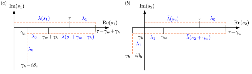
In order to obtain a perturbative expression of the CF given in Eq. (2), we utilize the Schwinger-Keldysh formal- ism, a systematic approach for calculating nonequilibrium Green’s functions and correlation functions under the influence of time-dependent perturbations by casting the problem on a closed time-ordered contour in the complex time plane, known as the Keldysh contour. For the problem considered here, all the unitary evolution operators and the exponential operators, e.g., e(iγwiγh)H(τ)e^{(i\gamma_{w}-i\gamma_{h})H(\tau)}, appearing in Eq. (2) are mapped on two modified Keldysh contours. The first trace in Eq. (2) corresponds to the modified contour CC, as shown in Fig. 2(a), and the second trace gives rise to another modified contour CC^{\prime}, as shown in Fig. 2(b). It is important to mention that, in the Schwinger-Keldysh formalism one typically expects closed contours while dealing with time-dependent perturbations. However, here, none of our modified contours are closed, only articulating the fact that both the traces that are mapped contain partial information about the non-unitary heat exchange stroke. The tails represent the presence of interaction H1H_{1} in the thermal states at AA and CC (see Fig. 1). We have demonstrated the details of this mapping in Appendix A and here we only provide a compact expression for the joint CF on the Keldysh contour,

χ(γw,γh)\displaystyle\chi(\gamma_{w},\gamma_{h}) =𝒯CeiCλC(s1)H1I(s1)𝑑s1β~c𝒯Ceiγhγhiβcλ0H1I(s1)𝑑s1βc\displaystyle=\frac{\big{\langle}{\cal T}_{C}\,e^{-\frac{i}{\hbar}\int_{C}\!\lambda_{C}(s_{1})H_{1}^{I}(s_{1})ds_{1}}\big{\rangle}_{\widetilde{\beta}_{c}}}{\big{\langle}{\cal T}_{C}\,e^{-\frac{i}{\hbar}\int_{\hbar\gamma_{h}}^{\hbar\gamma_{h}\!-\!i\hbar\beta_{c}}\!\lambda_{0}H_{1}^{I}(s_{1})ds_{1}}\big{\rangle}_{{\beta}_{c}}}
×𝒯CeiCλC(s2)H1I(s2)𝑑s2β~h𝒯Ceiτγhτγhiβhλ1H1I(s2)𝑑s2βh\displaystyle\times\,\frac{\big{\langle}{\cal T}_{C^{\prime}}\,e^{-\frac{i}{\hbar}\int_{C}\!{\lambda}_{C^{\prime}}(s_{2})H_{1}^{I}(s_{2})ds_{2}}\big{\rangle}_{\widetilde{\beta}_{h}}}{\big{\langle}{\cal T}_{C^{\prime}}\,e^{-\frac{i}{\hbar}\int_{\tau\!-\!\hbar\gamma_{h}}^{\tau\!-\!\hbar\gamma_{h}\!-\!i\hbar\beta_{h}}\!\lambda_{1}H_{1}^{I}(s_{2})ds_{2}}\big{\rangle}_{{\beta}_{h}}}
×eiγhH0βceiγhH0βh.\displaystyle\times\,\langle e^{-i\gamma_{h}H_{0}}\rangle_{\beta_{c}}\langle e^{i\gamma_{h}H_{0}}\rangle_{\beta_{h}}. (3)

Here, crucially, the averages in both the numerators are taken with respect to shifted inverse temperatures β~c=βc+iγh\widetilde{\beta}_{c}\!=\!\beta_{c}+i\gamma_{h} and β~h=βhiγh\widetilde{\beta}_{h}\!=\!{\beta}_{h}-i\gamma_{h} which are counting-field dependent. 𝒯C{\cal T}_{C} and 𝒯C{\cal T}_{C^{\prime}} are the contour-time ordered operators defined on the contours CC and CC^{\prime}, respectively, which orders the time-dependent operators according to their contour-time argument; i.e., sorting the operators from left to right with their contour-time arguments decreasing. In Appendix B we have expanded the exponential operators in Eq. (3) up to the second order in driving protocol λ(s)\lambda(s) and obtained the expression of the joint cumulant generating function (CGF) lnχ(γw,γh)\ln{\chi(\gamma_{w},\gamma_{h})} for arbitrary many-body working medium. The CGF is a useful quantity as it enables us to calculate all the cumulants (denoted by double angular brackets) of total work and heat exchange with the hot reservoir by taking partial derivatives with respect to γw\gamma_{w} and γh\gamma_{h}, respectively,

wkqhl=kl(iγw)k(iγh)llnχ(γw,γh)|γw,γh=0.\displaystyle\mathopen{\hbox{\set@color${\langle}$}\kern-1.94444pt\leavevmode\hbox{\set@color${\langle}$}}w^{k}q_{h}^{l}\mathclose{\hbox{\set@color${\rangle}$}\kern-1.94444pt\leavevmode\hbox{\set@color${\rangle}$}}=\frac{\partial^{k}\partial^{l}}{\partial(i\gamma_{w})^{k}\partial(i\gamma_{h})^{l}}\,\ln{\chi(\gamma_{w},\gamma_{h})}\Big{|}_{\gamma_{w},\gamma_{h}=0}. (4)
Refer to caption
Figure 2: The modified Keldysh contour to compute joint work and heat statistics for a generic quantum Otto cycle. (a)(a) Contour CC corresponds to the numerator of the first term in Eq. (2). Note that, the denominator of the first term runs only on the vertical tail as indicated by the integration limits. (b)(b) Contour CC^{\prime} corresponds to the numerator of the second term in Eq. (2). Here, we are considering symmetric driving only, i.e., 𝒰c=Θ𝒰eΘ\mathcal{U}_{c}=\Theta^{\dagger}\mathcal{U}_{e}^{\dagger}\Theta [or in other words λ~(s)=λ(τs)\tilde{\lambda}(s)\!=\!\lambda(\tau\!-\!s)]. The denominator of the second term runs only on the vertical tail as indicated by the integration limits. As mentioned in the main text, none of the modified contours CC and CC^{\prime} return to Re(s)=0\mathrm{Re}(s)\!=\!0 and get closed because of the presence of the non-unitary heat exchange stroke.

III Work and heat cumulants for arbitrary many-body working medium

In this section, we write down the final expression for the CGF valid up to the second order of the driving protocol λ(s)\lambda(s) (see Appendix B for the details). We obtain

lnχ(\displaystyle\ln\chi( γw,γh)=[iγw(λ1λ0)+iγhλ1][H1β~hH1β~c]+[iγw(λ12λ02)+iγhλ12]dω2πG~h>(ω)G~c>(ω)ω\displaystyle\gamma_{w},\gamma_{h})\!=\!\big{[}\!-\!i\gamma_{w}(\lambda_{1}\!-\!\lambda_{0})+i\gamma_{h}\lambda_{1}\big{]}\,\big{[}\langle H_{1}\rangle_{\widetilde{\beta}_{h}}\!\!-\!\langle H_{1}\rangle_{\widetilde{\beta}_{c}}\big{]}+\big{[}\!-\!i\hbar\gamma_{w}(\lambda_{1}^{2}\!-\!\lambda_{0}^{2})+i\hbar\gamma_{h}\lambda_{1}^{2}\big{]}\!\int\frac{d\omega}{2\pi}\frac{\widetilde{G}_{h}^{>}(\omega)\!-\!\widetilde{G}_{c}^{>}(\omega)}{\omega}
βcλ0[H1β~cH1βc+λ0dω2πG~c>(ω)Gc>(ω)ω]βhλ1[H1β~hH1βh+λ1dω2πG~h>(ω)Gh>(ω)ω]\displaystyle-\!\beta_{c}\lambda_{0}\Big{[}\langle H_{1}\rangle_{\widetilde{\beta}_{c}}\!\!-\!\langle H_{1}\rangle_{\beta_{c}}+\hbar\lambda_{0}\!\int\frac{d\omega}{2\pi}\frac{\widetilde{G}_{c}^{>}(\omega)\!-\!{G}_{c}^{>}(\omega)}{\omega}\Big{]}\!-\!\beta_{h}\lambda_{1}\Big{[}\langle H_{1}\rangle_{\widetilde{\beta}_{h}}\!\!-\!\langle H_{1}\rangle_{\beta_{h}}+\hbar\lambda_{1}\!\int\frac{d\omega}{2\pi}\frac{\widetilde{G}_{h}^{>}(\omega)\!-\!{G}_{h}^{>}(\omega)}{\omega}\Big{]}
+dω2π1eiω(γwγh)ω2A(ω)G~c>(ω)+dω2π1eiωγwω2A(ω)G~h>(ω)+lneiγhH0βc+lneiγhH0βh.\displaystyle+\!\int\frac{d\omega}{2\pi}\frac{1\!-\!e^{i\hbar\omega(\gamma_{w}\!-\!\gamma_{h})}}{\omega^{2}}A(\omega)\widetilde{G}_{c}^{>}(\omega)+\!\int\frac{d\omega}{2\pi}\frac{1\!-\!e^{i\hbar\omega\gamma_{w}}}{\omega^{2}}{A}(\omega)\widetilde{G}_{h}^{>}(\omega)+\ln{\langle e^{-i\gamma_{h}H_{0}}\rangle_{\beta_{c}}}+\ln{\langle e^{i\gamma_{h}H_{0}}\rangle_{\beta_{h}}}. (5)

Equation (5) is the first central result of this paper. It describes the statistical properties of total work and input heat fluctuations in the many-body Otto cycle in terms of one-point and two-point correlators of the interaction Hamiltonian H1H_{1}. In this expression, we suppress the integration limits for ω\omega, which ranges from -\infty to ++\infty. Here, the nonequilibrium Green’s functions are defined as connected two-point correlators of H1H_{1} in the interaction picture,

G~j>(s)\displaystyle\widetilde{G}_{j}^{>}(s) =(i)2H1I(s)H1β~j,\displaystyle=\left(\!-\frac{i}{\hbar}\right)^{2}\!\!\mathopen{\hbox{\set@color${\langle}$}\kern-1.94444pt\leavevmode\hbox{\set@color${\langle}$}}H_{1}^{I}(s)H_{1}\mathclose{\hbox{\set@color${\rangle}$}\kern-1.94444pt\leavevmode\hbox{\set@color${\rangle}$}}_{\widetilde{\beta}_{j}}, (6)
Gj>(s)\displaystyle{G}_{j}^{>}(s) =(i)2H1I(s)H1βj,\displaystyle=\left(\!-\frac{i}{\hbar}\right)^{2}\!\!\mathopen{\hbox{\set@color${\langle}$}\kern-1.94444pt\leavevmode\hbox{\set@color${\langle}$}}H_{1}^{I}(s)H_{1}\mathclose{\hbox{\set@color${\rangle}$}\kern-1.94444pt\leavevmode\hbox{\set@color${\rangle}$}}_{{\beta}_{j}}, (7)

where j=c,hj\!=\!c,h. In this context, \mathopen{\hbox{\set@color${\langle}$}\kern-1.94444pt\leavevmode\hbox{\set@color${\langle}$}}\cdot\mathclose{\hbox{\set@color${\rangle}$}\kern-1.94444pt\leavevmode\hbox{\set@color${\rangle}$}} implies a connected correlation function, also known as a cumulant correlation function,

XI(s1)YI(s2)β=XI(s1)YI(s2)βXβYβ.\mathopen{\hbox{\set@color${\langle}$}\kern-1.94444pt\leavevmode\hbox{\set@color${\langle}$}}X^{I}(s_{1})Y^{I}(s_{2})\mathclose{\hbox{\set@color${\rangle}$}\kern-1.94444pt\leavevmode\hbox{\set@color${\rangle}$}}_{\beta}=\langle X^{I}(s_{1})Y^{I}(s_{2})\rangle_{\beta}\!-\!\langle X\rangle_{\beta}\langle Y\rangle_{\beta}. (8)

The shifted inverse temperatures β~j\widetilde{\beta}_{j}, j=c,hj\!=\!c,h, appearing in Eq. (5) play a crucial role in calculating the cumulants of the heat exchange. In this paper, we adopt the Fourier transformation convention as

Gj>(ω)=+𝑑sGj>(s)eiωs.{G}_{j}^{>}(\omega)=\!\int_{-\infty}^{+\infty}\!\!ds\,{G}_{j}^{>}(s)\,e^{i\omega s}. (9)

Crucially, all the information about the time-dependent driving protocol is encapsulated in the quantity A(ω)A(\omega), defined as

A(ω)=|0τλ˙(t)eiωt𝑑t|2.\displaystyle A(\omega)=\left|\int_{0}^{\tau}\!\dot{\lambda}(t)e^{i\omega t}dt\right|^{2}. (10)

It is worth nothing that the CGF in Eq. (5) satisfies the normalization condition, lnχ(0,0)=0\ln{\chi(0,0)}\!=\!0. More importantly, it satisfies the universal heat engine fluctuation symmetry Campisi (2014); Campisi et al. (2015); Jarzynski and Wójcik (2004),

lnχ[iβc,i(βcβh)]=0.\ln\chi\big{[}i\beta_{c},\,i(\beta_{c}\!-\!\beta_{h})\big{]}=0. (11)

Notably, this fluctuation symmetry is a direct consequence of the Kubo-Martin-Schwinger (KMS) boundary condition satisfied by the Green’s functions introduced in Eqs. (6) and (7) Breuer and Petruccione (2002); Carmichael (1993); Kubo (1957); Martin and Schwinger (1959),

G~>(siβ~c)=G~>(s),\displaystyle\widetilde{G}^{>}(s\!-\!i\hbar\widetilde{\beta}_{c})=\widetilde{G}^{>}(-s), (12)
G>(siβc)=G>(s).\displaystyle{G}^{>}(s\!-\!i\hbar{\beta}_{c})={G}^{>}(-s). (13)

Here, β~c\widetilde{\beta}_{c} and βc{\beta}_{c} are the shifted and original inverse temperatures of the cold reservoir, respectively. Furthermore, the fluctuation symmetry in Eq. (11) implies that eΣ=1\langle e^{-\Sigma}\rangle\!=\!1, where Σ=βcw+(βcβh)qh\Sigma\!=\!\beta_{c}w+(\beta_{c}\!-\!\beta_{h})q_{h} is the stochastic entropy production in a single cycle. It is worth highlighting that utilizing Jensen’s inequality, eΣeΣ\langle e^{-\Sigma}\rangle\geq e^{-\langle\Sigma\rangle}, we immediately recover the second law of thermodynamics, Σ0\langle\Sigma\rangle\geq 0 Landi and Paternostro (2021).

In the following, we present the formal expressions of the first and second cumulants of total work and heat exchange with the hot reservoir. The average total work is given by

w=\displaystyle\langle w\rangle\!= (λ1λ0)[H1βhH1βc]\displaystyle-\!(\lambda_{1}\!-\!\lambda_{0})\left[\langle H_{1}\rangle_{\beta_{h}}\!\!-\!\langle H_{1}\rangle_{\beta_{c}}\right]
(λ12λ02)dω2π1ω[Gh>(ω)Gc>(ω)]\displaystyle-\hbar(\lambda_{1}^{2}\!-\!\lambda_{0}^{2})\!\int\!\frac{d\omega}{2\pi}\frac{1}{\omega}\left[{G}_{h}^{>}(\omega)\!-\!{G}_{c}^{>}(\omega)\right]
dω2πA(ω)ω[Gc>(ω)+Gh>(ω)].\displaystyle-\!\hbar\!\int\!\frac{d\omega}{2\pi}\frac{A(\omega)}{\omega}\left[G^{>}_{c}(\omega)+G^{>}_{h}(\omega)\right]. (14)

The first two terms on the right-hand side represent the boundary terms that depend on the end values of the driving protocol and are associated with the total change in free energy during the two unitary work strokes.

The corresponding variance (second cumulant) of total work is given by

w2=2dω2πA(ω)[Gc>(ω)+Gh>(ω)].\mathopen{\hbox{\set@color${\langle}$}\kern-1.94444pt\leavevmode\hbox{\set@color${\langle}$}}w^{2}\mathclose{\hbox{\set@color${\rangle}$}\kern-1.94444pt\leavevmode\hbox{\set@color${\rangle}$}}=-\hbar^{2}\!\int\!\frac{d\omega}{2\pi}A(\omega)\left[G^{>}_{c}(\omega)+G^{>}_{h}(\omega)\right]. (15)

Notably, we find that calculating the cumulants of heat exchange qhq_{h} requires more involved calculations due to the presence of shifted inverse temperatures β~c\widetilde{\beta}_{c} and β~h\widetilde{\beta}_{h}. This results in connected correlators of the form H1H0\mathopen{\hbox{\set@color${\langle}$}\kern-1.94444pt\leavevmode\hbox{\set@color${\langle}$}}H_{1}H_{0}\mathclose{\hbox{\set@color${\rangle}$}\kern-1.94444pt\leavevmode\hbox{\set@color${\rangle}$}}, H1I(s)H1H0\mathopen{\hbox{\set@color${\langle}$}\kern-1.94444pt\leavevmode\hbox{\set@color${\langle}$}}H_{1}^{I}(s)H_{1}H_{0}\mathclose{\hbox{\set@color${\rangle}$}\kern-1.94444pt\leavevmode\hbox{\set@color${\rangle}$}}, and so on. We note that, for an arbitrary operator XX,

dd(iγh)Xβ~j=XH0β~j,\displaystyle\frac{d}{d(i\gamma_{h})}\langle X\rangle_{\widetilde{\beta}_{j}}\!=\!\mp\mathopen{\hbox{\set@color${\langle}$}\kern-1.94444pt\leavevmode\hbox{\set@color${\langle}$}}XH_{0}\mathclose{\hbox{\set@color${\rangle}$}\kern-1.94444pt\leavevmode\hbox{\set@color${\rangle}$}}_{\widetilde{\beta}_{j}}, (16)
d2d(iγh)2Xβ~j=XH02β~j,\displaystyle\frac{d^{2}}{d(i\gamma_{h})^{2}}\langle X\rangle_{\widetilde{\beta}_{j}}\!=\!\mathopen{\hbox{\set@color${\langle}$}\kern-1.94444pt\leavevmode\hbox{\set@color${\langle}$}}XH_{0}^{2}\mathclose{\hbox{\set@color${\rangle}$}\kern-1.94444pt\leavevmode\hbox{\set@color${\rangle}$}}_{\widetilde{\beta}_{j}}, (17)

where ()(\!-\!) corresponds to j=cj\!=\!c, and (+)(+) corresponds to j=hj\!=\!h, respectively. Below we list the expressions for the average heat exchange with the hot reservoir and its variance,

qh=\displaystyle\langle q_{h}\rangle\!= H0βhH0βc+λ1[H1βhH1βc]+λ12dω2πGh>(ω)Gc>(ω)ω+βcλ0[H0H1βc+λ0dω2πGc(ω)ω]\displaystyle\langle H_{0}\rangle_{\beta_{h}}\!\!-\!\langle H_{0}\rangle_{\beta_{c}}+\lambda_{1}\big{[}\langle H_{1}\rangle_{\beta_{h}}\!\!-\!\langle H_{1}\rangle_{\beta_{c}}\big{]}+\hbar\lambda_{1}^{2}\!\int\!{\frac{d\omega}{2\pi}\frac{{G}_{h}^{>}(\omega)\!-\!{G}_{c}^{>}(\omega)}{\omega}}+\beta_{c}\lambda_{0}\Big{[}\mathopen{\hbox{\set@color${\langle}$}\kern-1.94444pt\leavevmode\hbox{\set@color${\langle}$}}H_{0}H_{1}\mathclose{\hbox{\set@color${\rangle}$}\kern-1.94444pt\leavevmode\hbox{\set@color${\rangle}$}}_{\beta_{c}}\!+\hbar\lambda_{0}\!\int\!\frac{d\omega}{2\pi}\frac{G^{{}^{\prime}}_{c}(\omega)}{\omega}\Big{]}
βhλ1[H0H1βh+λ1dω2πGh(ω)ω]+dω2πA(ω)Gc>(ω)ω,\displaystyle\quad\quad\quad\quad-\!\beta_{h}\lambda_{1}\Big{[}\mathopen{\hbox{\set@color${\langle}$}\kern-1.94444pt\leavevmode\hbox{\set@color${\langle}$}}H_{0}H_{1}\mathclose{\hbox{\set@color${\rangle}$}\kern-1.94444pt\leavevmode\hbox{\set@color${\rangle}$}}_{\beta_{h}}\!+\hbar\lambda_{1}\!\int\!\frac{d\omega}{2\pi}\frac{G^{{}^{\prime}}_{h}(\omega)}{\omega}\Big{]}+\hbar\!\int\!\frac{d\omega}{2\pi}\frac{A(\omega)G^{>}_{c}(\omega)}{\omega}, (18)
qh2=\displaystyle\mathopen{\hbox{\set@color${\langle}$}\kern-1.94444pt\leavevmode\hbox{\set@color${\langle}$}}q_{h}^{2}\mathclose{\hbox{\set@color${\rangle}$}\kern-1.94444pt\leavevmode\hbox{\set@color${\rangle}$}}\!= H02βc+H02βh+2λ1[H0H1βc+H0H1βh]+2λ12dωπGc(ω)+Gh(ω)ωβcλ0[H02H1βc\displaystyle\mathopen{\hbox{\set@color${\langle}$}\kern-1.94444pt\leavevmode\hbox{\set@color${\langle}$}}H_{0}^{2}\mathclose{\hbox{\set@color${\rangle}$}\kern-1.94444pt\leavevmode\hbox{\set@color${\rangle}$}}_{\beta_{c}}\!+\mathopen{\hbox{\set@color${\langle}$}\kern-1.94444pt\leavevmode\hbox{\set@color${\langle}$}}H_{0}^{2}\mathclose{\hbox{\set@color${\rangle}$}\kern-1.94444pt\leavevmode\hbox{\set@color${\rangle}$}}_{\beta_{h}}\!+2\lambda_{1}\big{[}\mathopen{\hbox{\set@color${\langle}$}\kern-1.94444pt\leavevmode\hbox{\set@color${\langle}$}}H_{0}H_{1}\mathclose{\hbox{\set@color${\rangle}$}\kern-1.94444pt\leavevmode\hbox{\set@color${\rangle}$}}_{\beta_{c}}\!+\mathopen{\hbox{\set@color${\langle}$}\kern-1.94444pt\leavevmode\hbox{\set@color${\langle}$}}H_{0}H_{1}\mathclose{\hbox{\set@color${\rangle}$}\kern-1.94444pt\leavevmode\hbox{\set@color${\rangle}$}}_{\beta_{h}}\big{]}+2\hbar\lambda_{1}^{2}\int\!\frac{d\omega}{\pi}\frac{G_{c}^{{}^{\prime}}(\omega)+G_{h}^{{}^{\prime}}(\omega)}{\omega}\!-\!\beta_{c}\lambda_{0}\Big{[}\mathopen{\hbox{\set@color${\langle}$}\kern-1.94444pt\leavevmode\hbox{\set@color${\langle}$}}H_{0}^{2}H_{1}\mathclose{\hbox{\set@color${\rangle}$}\kern-1.94444pt\leavevmode\hbox{\set@color${\rangle}$}}_{\beta_{c}}
+λ0dω2πGc′′(ω)ω]βhλ1[H02H1βh+λ1dω2πGh′′(ω)ω]+2dω2πGc(ω)A(ω)ω+2dω2πA(ω)Gc>(ω),\displaystyle\!\!+\hbar\lambda_{0}\!\int\!\frac{d\omega}{2\pi}\frac{G_{c}^{{}^{\prime\prime}}(\omega)}{\omega}\Big{]}\!-\!\beta_{h}\lambda_{1}\Big{[}\mathopen{\hbox{\set@color${\langle}$}\kern-1.94444pt\leavevmode\hbox{\set@color${\langle}$}}H_{0}^{2}H_{1}\mathclose{\hbox{\set@color${\rangle}$}\kern-1.94444pt\leavevmode\hbox{\set@color${\rangle}$}}_{\beta_{h}}\!+\hbar\lambda_{1}\!\int\!\frac{d\omega}{2\pi}\frac{G_{h}^{{}^{\prime\prime}}(\omega)}{\omega}\Big{]}+2\hbar\!\int\!\frac{d\omega}{2\pi}\frac{G^{{}^{\prime}}_{c}(\omega)A(\omega)}{\omega}+\hbar^{2}\!\int\!\frac{d\omega}{2\pi}{A(\omega)G_{c}^{>}(\omega)}, (19)

where we have introduced a compact notation,

Gj(ω)\displaystyle G_{j}^{{}^{\prime}}(\omega) =\displaystyle= βjGj>(ω),\displaystyle-\frac{\partial}{\partial\beta_{j}}G_{j}^{>}(\omega), (20)
Gj′′(ω)\displaystyle G_{j}^{{}^{\prime\prime}}(\omega) =\displaystyle= 2βj2Gj>(ω),\displaystyle\frac{\partial^{2}}{\partial\beta_{j}^{2}}G_{j}^{>}(\omega), (21)

with j=c,hj=c,h.

Now that we have obtained the expressions for the mean and the variance for total work and heat exchange with the hot reservoir from the joint CGF, in the following section, we focus on establishing the linear response regime for the generic quantum Otto cycle. We derive the expressions for Onsager’s transport coefficients and explore the fate of traditional fluctuation-dissipation relations for work and heat.

IV Linear response, Onsager coefficients, and universal bounds

Let us first parameterize the driving protocol λ(t)\lambda(t) as

λ(t)=λ+Δλf(t),\displaystyle\lambda(t)=\lambda+\Delta\lambda\,f(t), (22)

where, λ=λ0\lambda\!=\!\lambda_{0} and Δλ=λ1λ0\Delta\lambda\!=\!\lambda_{1}\!-\!\lambda_{0}. The function f(t)f(t) is defined such that f(0)=0f(0)\!=\!0 and f(τ)=1f(\tau)\!=\!1 to ensure that λ0\lambda_{0} and λ1\lambda_{1} are the boundary values of the protocol λ(t)\lambda(t) at time t=0t\!=\!0 and time t=τt\!=\!\tau, respectively. Recall that τ\tau is the duration of each work stroke. To identify the proper thermodynamic affinities and the corresponding conjugate fluxes, we begin with the definition of the stochastic entropy production in a single cycle:

Σ=\displaystyle\Sigma= βcw+(βcβh)qh\displaystyle\beta_{c}w+(\beta_{c}\!-\!\beta_{h})\,q_{h}
=\displaystyle= (βcΔλ)wΔλ+(βcβh)qh.\displaystyle\bm{(}\beta_{c}\Delta\lambda\bm{)}\frac{w}{\Delta\lambda}+\bm{(}\beta_{c}\!-\!\beta_{h}\bm{)}q_{h}. (23)

From this expression, we can identify the thermodynamic affinities as w=βcΔλ{\cal F}_{w}\!=\!\beta_{c}\Delta\lambda and q=βcβh{\cal F}_{q}\!=\!\beta_{c}\!-\!\beta_{h}, and the corresponding integrated work and heat fluxes as w/Δλw/\Delta\lambda and qhq_{h}, respectively. One can further define the heat and work currents by dividing the integrated heat and work fluxes with total cycle time τcyc=2τ+τh+τc\tau_{cyc}\!=\!2\tau+\tau_{h}+\tau_{c}, as follows:

𝒥w=1τcycwΔλand𝒥h=qhτcyc.\displaystyle\;\;\mathcal{J}_{w}\!=\!\frac{1}{\tau_{cyc}}\frac{w}{\Delta\lambda}\;\;\mathrm{and}\;\;\mathcal{J}_{h}\!=\!\frac{q_{h}}{\tau_{cyc}}. (24)

Consequently, the average entropy production rate in one complete cycle σ=Σ/τcyc\langle\sigma\rangle\!=\!\langle\Sigma\rangle/\tau_{cyc} can be expressed as

σ=i𝒥ii,\displaystyle\langle\sigma\rangle=\sum_{i}\langle\mathcal{J}_{i}\rangle\mathcal{F}_{i}, (25)

where i=w,hi\!=\!w,h. From this point onwards, we adopt βc=β\beta_{c}\!=\!\beta and βcβh=Δβ\beta_{c}\!-\!\beta_{h}\!=\!\Delta\beta, and focus on the linear response regime where Δββ\Delta\beta\ll\beta. In this regime, we can effectively utilize the following expansion,

XβΔβ=\displaystyle\langle X\rangle_{\beta\!-\!\Delta\beta}= XβΔββXβ\displaystyle\langle X\rangle_{\beta}\!-\!\Delta\beta\,\frac{\partial}{\partial\beta}\langle X\rangle_{\beta}
=\displaystyle= Xβ+ΔβXH0β.\displaystyle\langle X\rangle_{\beta}+\Delta\beta\mathopen{\hbox{\set@color${\langle}$}\kern-1.94444pt\leavevmode\hbox{\set@color${\langle}$}}XH_{0}\mathclose{\hbox{\set@color${\rangle}$}\kern-1.94444pt\leavevmode\hbox{\set@color${\rangle}$}}_{\beta}. (26)

Note that the appearance of the free Hamiltonian H0H_{0} in the second term arises from the derivative with respect to β\beta over a canonical distribution characterized by eβH0/Tr[eβH0]e^{-\beta H_{0}}/\operatorname{Tr}{[e^{-\beta H_{0}}]}. To proceed with our linear response analysis for the generic Otto cycle, we calculate the average work and heat fluxes, 𝒥w\langle\mathcal{J}_{w}\rangle and 𝒥h\langle\mathcal{J}_{h}\rangle, using Eqs. (14) and (18), respectively, which are accurate up to the second order of the driving protocol λ(t)\lambda(t). Finally, carrying out the Taylor expansion given in Eq. (26) and keeping terms up to the linear order of the affinities, w\mathcal{F}_{w} and q\mathcal{F}_{q}, we derive the following relation between the currents and affinities, connected via the Onsager matrix:

(𝒥w𝒥h)=(wwwqqwqq)(wq),\displaystyle\begin{pmatrix}\langle\mathcal{J}_{w}\rangle\\ \langle\mathcal{J}_{h}\rangle\end{pmatrix}=\begin{pmatrix}{\cal L}_{ww}&{\cal L}_{wq}\\ {\cal L}_{qw}&{\cal L}_{qq}\end{pmatrix}\begin{pmatrix}{\cal F}_{w}\\ {\cal F}_{q}\end{pmatrix}, (27)

where the Onsager transport coefficients ij{\cal L}_{ij}, with i,j=w,qi,j=w,q, are given by

ww\displaystyle{\cal L}_{ww}\! =1τcycdω2π2F(ω)G>(ω)βω,\displaystyle=\!-\frac{1}{\tau_{cyc}}\hbar\!\int\!\frac{d\omega}{2\pi}\frac{2F(\omega)G^{>}(\omega)}{\beta\,\omega}, (28)
wq\displaystyle{\cal L}_{wq}\! =qw=1τcycβ[H1β+2λdω2πG>(ω)ω],\displaystyle=\!{\cal L}_{qw}\!=\!\frac{1}{\tau_{cyc}}\frac{\partial}{\partial\beta}\Big{[}\langle H_{1}\rangle_{\beta}\!+\!2\hbar\lambda\!\!\int\!\frac{d\omega}{2\pi}\frac{G^{>}(\omega)}{\omega}\Big{]}, (29)
qq\displaystyle\mathcal{L}_{qq}\! =β[H0β+λβ(βH1β+λβdω2πG>(ω)ω)].\displaystyle=\!-\frac{\partial}{\partial\beta}\Big{[}\langle H_{0}\rangle_{\beta}\!+\!\lambda\frac{\partial}{\partial\beta}\Big{(}\beta\langle H_{1}\rangle_{\beta}\!+\hbar\lambda\beta\!\!\int\!\frac{d\omega}{2\pi}\frac{G^{>}(\omega)}{\omega}\Big{)}\Big{]}. (30)

Here, note that

F(ω)=|0τf˙(t)eiωt𝑑t|2=A(ω)Δλ2\displaystyle F(\omega)=\left|\int_{0}^{\tau}\!\dot{f}(t)e^{i\omega t}dt\right|^{2}\!=\frac{A(\omega)}{{\Delta\lambda}^{2}} (31)

encodes the information of driving where Δλ\Delta\lambda and f(t)f(t) are defined in Eq. (22). The Green’s function G>(ω)G^{>}(\omega) is evaluated at the equilibrium temperature β\beta. Importantly, we recover the Onsager reciprocity relation Onsager (1931), i.e. wq=qw\mathcal{L}_{wq}\!=\!\mathcal{L}_{qw}, as shown in Eq. (29). The derived expressions for the Onsager transport coefficients, characterizing the behavior of an arbitrary working medium executing the Otto cycle in the linear response regime, constitute another central result of our work. With these results in hand, we proceed to provide some important insights and remarks.

The traditional “Fluctuation-Dissipation relations” (FDRs) typically connect the diagonal elements of the Onsager matrix to equilibrium fluctuations Kubo (1966). Remarkably, in our analysis, we precisely recover the traditional FDR for the heat current 𝒥h\langle\mathcal{J}_{h}\rangle (detailed derivation in Appendix E),

qq=𝒥h22|w,q=0,\displaystyle{{\cal L}_{qq}}=\frac{\mathopen{\hbox{\set@color${\langle}$}\kern-1.94444pt\leavevmode\hbox{\set@color${\langle}$}}\mathcal{J}_{h}^{2}\mathclose{\hbox{\set@color${\rangle}$}\kern-1.94444pt\leavevmode\hbox{\set@color${\rangle}$}}}{2}\bigg{|}_{\mathcal{F}_{w},\mathcal{F}_{q}=0}, (32)

where we recall that 𝒥h2=qh2/τcyc\mathopen{\hbox{\set@color${\langle}$}\kern-1.94444pt\leavevmode\hbox{\set@color${\langle}$}}\mathcal{J}_{h}^{2}\mathclose{\hbox{\set@color${\rangle}$}\kern-1.94444pt\leavevmode\hbox{\set@color${\rangle}$}}\!=\!\mathopen{\hbox{\set@color${\langle}$}\kern-1.94444pt\leavevmode\hbox{\set@color${\langle}$}}q_{h}^{2}\mathclose{\hbox{\set@color${\rangle}$}\kern-1.94444pt\leavevmode\hbox{\set@color${\rangle}$}}/\tau_{cyc}. However, importantly, the same is not true for the case of work current. In fact, for the work current fluctuation, following Eq. (15), we obtain

𝒥w22|w,q=0=1τcyc2dω2πF(ω)G>(ω),\displaystyle\frac{\mathopen{\hbox{\set@color${\langle}$}\kern-1.94444pt\leavevmode\hbox{\set@color${\langle}$}}\mathcal{J}_{w}^{2}\mathclose{\hbox{\set@color${\rangle}$}\kern-1.94444pt\leavevmode\hbox{\set@color${\rangle}$}}}{2}\bigg{|}_{\mathcal{F}_{w},\mathcal{F}_{q}=0}=-\frac{1}{\tau_{cyc}}\hbar^{2}\!\int\!\frac{d\omega}{2\pi}F(\omega)G^{>}(\omega), (33)

which does not match the diagonal Onsager coefficient ww\mathcal{L}_{ww}. To investigate this discrepancy further, let us rewrite the expressions for ww\mathcal{L}_{ww} and 𝒥w2\mathopen{\hbox{\set@color${\langle}$}\kern-1.94444pt\leavevmode\hbox{\set@color${\langle}$}}\mathcal{J}_{w}^{2}\mathclose{\hbox{\set@color${\rangle}$}\kern-1.94444pt\leavevmode\hbox{\set@color${\rangle}$}} as follows:

ww=1τcyc22dω2πF(ω)tanh(βω2)βω2[G>(ω)+G>(ω)].\displaystyle{\cal L}_{ww}\!=\!-\frac{1}{\tau_{cyc}}\frac{\hbar^{2}}{2}\!\!\int\!\frac{d\omega}{2\pi}F(\omega)\frac{\tanh{\big{(}\frac{\beta\hbar\omega}{2}\big{)}}}{\frac{\beta\hbar\omega}{2}}\big{[}G^{>}(\omega)+G^{>}(\!-\omega)\big{]}. (34)
𝒥w22|w,q=0=1τcyc22dω2πF(ω)[G>(ω)+G>(ω)],\displaystyle\frac{\mathopen{\hbox{\set@color${\langle}$}\kern-1.94444pt\leavevmode\hbox{\set@color${\langle}$}}\mathcal{J}_{w}^{2}\mathclose{\hbox{\set@color${\rangle}$}\kern-1.94444pt\leavevmode\hbox{\set@color${\rangle}$}}}{2}\bigg{|}_{\mathcal{F}_{w},\mathcal{F}_{q}=0}\!=\!\!-\frac{1}{\tau_{cyc}}\frac{\hbar^{2}}{2}\!\int\!\frac{d\omega}{2\pi}F(\omega)\big{[}G^{>}(\omega)+G^{>}(\!-\omega)\big{]}, (35)

Here, we have utilized an important identity involving the Green’s functions,

G>(ω)G>(ω)=tanh(βω2)[G>(ω)+G>(ω)].G^{>}(\omega)\!-\!G^{>}(\!-\omega)=\tanh{\Big{(}\frac{\beta\hbar\omega}{2}\Big{)}}\big{[}G^{>}(\omega)+G^{>}(\!-\omega)\big{]}. (36)

which arises from the KMS condition in the Fourier space, eβωG>(ω)=G>(ω)e^{-\beta\hbar\omega}G^{>}(\omega)\!=\!G^{>}(-\omega). Now, considering the fact that tanh(x)/x1{\tanh{(x)}}/{x}\!\leq\!1, we deduce from Eqs. (35) and (34) that

ww𝒥w22|w,q=0,\displaystyle{\cal L}_{ww}\leq\frac{\mathopen{\hbox{\set@color${\langle}$}\kern-1.94444pt\leavevmode\hbox{\set@color${\langle}$}}\mathcal{J}_{w}^{2}\mathclose{\hbox{\set@color${\rangle}$}\kern-1.94444pt\leavevmode\hbox{\set@color${\rangle}$}}}{2}\bigg{|}_{\mathcal{F}_{w},\mathcal{F}_{q}=0}, (37)

highlighting a breakdown of the traditional FDR for work current. Importantly, this breakdown is purely of quantum origin, and the equality is restored in the quantum-adiabatic limit, i.e., when [H0,H1]=0[H_{0},H_{1}]\!=\!0. This observation aligns with the recent findings of Ref. Miller et al., 2019; Scandi et al., 2020 where a similar breakdown was reported.

The obtained results for the Onsager coefficients and the FDR breakdown for work current have remarkable implications in determining the universal bounds on the performance of the quantum Otto cycle operating as an engine or refrigerator. Particularly, it is noteworthy that the thermodynamic uncertainty relation Sacchi (2021a, b) holds for the currents 𝒥w\langle\mathcal{J}_{w}\rangle and 𝒥h\langle\mathcal{J}_{h}\rangle, as shown in Appendix D,

σ𝒥w2𝒥w22,σ𝒥h2𝒥h22,\displaystyle\langle\sigma\rangle\frac{\mathopen{\hbox{\set@color${\langle}$}\kern-1.94444pt\leavevmode\hbox{\set@color${\langle}$}}\mathcal{J}_{w}^{2}\mathclose{\hbox{\set@color${\rangle}$}\kern-1.94444pt\leavevmode\hbox{\set@color${\rangle}$}}}{\langle\mathcal{J}_{w}\rangle^{2}}\geq 2,\quad\langle\sigma\rangle\frac{\mathopen{\hbox{\set@color${\langle}$}\kern-1.94444pt\leavevmode\hbox{\set@color${\langle}$}}\mathcal{J}_{h}^{2}\mathclose{\hbox{\set@color${\rangle}$}\kern-1.94444pt\leavevmode\hbox{\set@color${\rangle}$}}}{\langle\mathcal{J}_{h}\rangle^{2}}\geq 2, (38)

where σ=Σ/τcyc\langle\sigma\rangle=\langle\Sigma\rangle/\tau_{\textrm{cyc}} represents average entropy production rate. Notably, these TURs remain valid independently of the nature of the Otto cycle’s operation, i.e., whether it acts as an engine, refrigerator, heater, or accelerator Solfanelli et al. (2020).

Let us now focus on understanding bounds on nonequilibrium fluctuations when the Otto cycle works as an engine, i.e., converting a fraction of spontaneous heat flux flowing from hot to cold reservoir into useful work. To quantify the engine’s performance, we introduce the power output as

𝒫=w/τcyc=wβ𝒥w\langle\mathcal{P}\rangle=-\langle w\rangle/\tau_{cyc}=\!-\frac{{\cal F}_{w}}{\beta}\langle\mathcal{J}_{w}\rangle (39)

and the input heat current is given by 𝒥h\langle\mathcal{J}_{h}\rangle. The engine operational regime of the Otto cycle is characterized by 𝒫>0\langle\mathcal{P}\rangle\!>\!0, and 𝒥h>0\langle\mathcal{J}_{h}\rangle\!>\!0, as per our sign convention where energy flowing into the working fluid is considered positive. To achieve this, the necessary requirement is q>w\mathcal{F}_{q}\!>\!\mathcal{F}_{w}. Following the second law of thermodynamics, σ0\langle\sigma\rangle\!\geq\!0, it is straightforward to show that the average efficiency of the Otto engine, η𝒫/𝒥h\langle\eta\rangle\!\coloneqq\!\langle\mathcal{P}\rangle/\langle\mathcal{J}_{h}\rangle, is universally upper bounded by the the Carnot bound ηc=Δβ/β\eta_{c}\!=\!\Delta\beta/\beta Callen et al. (1985); Lieb and Yngvason (1999), ηηc\langle\eta\rangle\!\leq\!\eta_{c}. In order to derive bounds on nonequilibrium fluctuations, following Ref. Saryal et al. (2021), we construct the quantity η(2)\eta^{(2)}, which is the ratio of power fluctuation to the fluctuation of input heat current,

η(2)=𝒫2𝒥h2.\displaystyle\eta^{(2)}=\frac{\mathopen{\hbox{\set@color${\langle}$}\kern-1.94444pt\leavevmode\hbox{\set@color${\langle}$}}\mathcal{P}^{2}\mathclose{\hbox{\set@color${\rangle}$}\kern-1.94444pt\leavevmode\hbox{\set@color${\rangle}$}}}{\mathopen{\hbox{\set@color${\langle}$}\kern-1.94444pt\leavevmode\hbox{\set@color${\langle}$}}\mathcal{J}_{h}^{2}\mathclose{\hbox{\set@color${\rangle}$}\kern-1.94444pt\leavevmode\hbox{\set@color${\rangle}$}}}. (40)

Recently, it was shown that in the case of a continuously coupled autonomous steady-state heat engine operating in the linear response regime, where both the work and heat FDRs are valid, the ratio of output power to input heat current fluctuations is subject to both universal lower and upper bounds Saryal et al. (2021),

η2[η(2)]autoηc2,\displaystyle\langle\eta\rangle^{2}\leq\big{[}\eta^{(2)}\big{]}_{\mathrm{auto}}\leq\eta_{c}^{2}, (41)

where the subscript ‘auto\mathrm{auto}’ stands for the autonomous steady-state heat engine. However, in our case of a generic finite-time Otto engine operating in the linear response limit, we obtain the following inequality (see Appendix E for details),

ηc2w2wwβ2qqη2.\eta_{c}^{2}\geq\frac{{\cal F}_{w}^{2}{\cal L}_{ww}}{\beta^{2}{\cal L}_{qq}}\geq\langle\eta\rangle^{2}. (42)

A key point to note here is that, contrary to the autonomous steady-state engine, we observe a violation of the traditional work FDR in the discrete Otto cycle, as given in Eq. (37). This FDR breakdown for the work current leads to the following inequality:

η(2)w2wwβ2qq.\displaystyle\eta^{(2)}\geq\frac{{\cal F}_{w}^{2}{\cal L}_{ww}}{\beta^{2}{\cal L}_{qq}}. (43)

Importantly, the equality is restored when the driving Hamiltonian H1H_{1} commutes with the free Hamiltonian H0H_{0}, i.e., in the quantum-adiabatic driving limit. As an immediate consequence of the inequality in Eq. (43), the lower bound on η(2)\eta^{(2)} remains robust,

η(2)η2.\displaystyle\eta^{(2)}\geq\langle\eta\rangle^{2}. (44)

However, the upper bound on η(2)\eta^{(2)} may not always hold true, i.e., η(2)ηc2\eta^{(2)}\nleq\eta_{c}^{2}, the reason being purely of quantum origin. This distinction is a significant departure from the autonomous case, where both the lower and upper bounds remain intact. In the Otto cycle, due to the violation of the traditional work FDR, the upper bound is not guaranteed, highlighting the impact of nonequilibrium and quantum effects on the engine’s performance. This constitutes another central result of this work. As a direct consequence of the lower bound for η(2)\eta^{(2)} in Eq. (44), a hierarchical relation between the TURs is observed. This follows from the fact that

η(2)η2𝒥w2𝒥w2𝒥h2𝒥h2.\eta^{(2)}\!\geq\!\langle\eta\rangle^{2}\Rightarrow\frac{\mathopen{\hbox{\set@color${\langle}$}\kern-1.94444pt\leavevmode\hbox{\set@color${\langle}$}}\mathcal{J}_{w}^{2}\mathclose{\hbox{\set@color${\rangle}$}\kern-1.94444pt\leavevmode\hbox{\set@color${\rangle}$}}}{\langle\mathcal{J}_{w}\rangle^{2}}\!\geq\!\frac{\mathopen{\hbox{\set@color${\langle}$}\kern-1.94444pt\leavevmode\hbox{\set@color${\langle}$}}\mathcal{J}_{h}^{2}\mathclose{\hbox{\set@color${\rangle}$}\kern-1.94444pt\leavevmode\hbox{\set@color${\rangle}$}}}{\langle\mathcal{J}_{h}\rangle^{2}}. (45)

As a result, in the engine regime, a strict hierarchy between the TURs of work (output) and heat (input) currents is obtained:

σ𝒥w2𝒥w2σ𝒥h2𝒥h22.\displaystyle\langle\sigma\rangle\frac{\mathopen{\hbox{\set@color${\langle}$}\kern-1.94444pt\leavevmode\hbox{\set@color${\langle}$}}\mathcal{J}_{w}^{2}\mathclose{\hbox{\set@color${\rangle}$}\kern-1.94444pt\leavevmode\hbox{\set@color${\rangle}$}}}{\langle\mathcal{J}_{w}\rangle^{2}}\geq\langle\sigma\rangle\frac{\mathopen{\hbox{\set@color${\langle}$}\kern-1.94444pt\leavevmode\hbox{\set@color${\langle}$}}\mathcal{J}_{h}^{2}\mathclose{\hbox{\set@color${\rangle}$}\kern-1.94444pt\leavevmode\hbox{\set@color${\rangle}$}}}{\langle\mathcal{J}_{h}\rangle^{2}}\!\geq\!2. (46)

After our exploration of the engine regime, we now shift our focus to the refrigerator regime. In this mode of operation, the primary objective is to extract heat from the cold reservoir by utilizing external work. Following our sign convention, i.e., energy entering the working fluid is considered positive, the refrigerator regime is characterized by a positive current flowing out of the cold reservoir, 𝒥c>0\langle\mathcal{J}_{c}\rangle\!>\!0, and work is performed on the system, 𝒥w>0\langle\mathcal{J}_{w}\rangle\!>\!0. To achieve refrigeration, it is necessary that the affinities satisfy w>q\mathcal{F}_{w}\!>\!\mathcal{F}_{q}. The performance of the refrigerator is quantified by its coefficient of performance (COP), denoted as ε\langle\varepsilon\rangle. Notably, the COP of a refrigerator is universally upper bounded by the Carnot COP Callen et al. (1985); Abah and Lutz (2016), i.e.,

εβ𝒥cw𝒥wεc,\displaystyle\langle\varepsilon\rangle\coloneqq\frac{\beta\langle\mathcal{J}_{c}\rangle}{\mathcal{F}_{w}\langle\mathcal{J}_{w}\rangle}\leq\varepsilon_{c}, (47)

where εc=(1ηc)/ηcβ/Δβ\varepsilon_{c}\!=\!(1-\eta_{c})/\eta_{c}\approx\beta/\Delta\beta. Let us now investigate the quantity ε(2)\varepsilon^{(2)} defined as

ε(2)β2𝒥c2w2𝒥w2.\displaystyle\varepsilon^{(2)}\coloneqq\frac{\beta^{2}\mathopen{\hbox{\set@color${\langle}$}\kern-1.94444pt\leavevmode\hbox{\set@color${\langle}$}}\mathcal{J}_{c}^{2}\mathclose{\hbox{\set@color${\rangle}$}\kern-1.94444pt\leavevmode\hbox{\set@color${\rangle}$}}}{\mathcal{F}_{w}^{2}\mathopen{\hbox{\set@color${\langle}$}\kern-1.94444pt\leavevmode\hbox{\set@color${\langle}$}}\mathcal{J}_{w}^{2}\mathclose{\hbox{\set@color${\rangle}$}\kern-1.94444pt\leavevmode\hbox{\set@color${\rangle}$}}}. (48)

In Appendix F we have derived the expression of CGF for the heat extracted from the cold reservoir, from which we can obtain the expressions for the average heat extracted and its variance. It is worth mentioning that for steady-state autonomous refrigerators operating in the linear response regime, the quantity ε(2)\varepsilon^{(2)} was reported to possess both universal upper and lower bounds Mohanta et al. (2022),

εc2[ε(2)]autoε2.\varepsilon_{c}^{2}\geq\big{[}\varepsilon^{(2)}\big{]}_{\mathrm{auto}}\geq\langle\varepsilon\rangle^{2}. (49)

where, recall that the subscript ‘auto\mathrm{auto}’ denotes the autonomous steady-state refrigerator. In our case of a generic Otto cycle operating as a refrigerator, we derived the following inequality (see Appendix G for details):

εc2β2qqw2wwε2.\varepsilon_{c}^{2}\geq\frac{\beta^{2}{\cal L}_{qq}}{{\cal F}_{w}^{2}{\cal L}_{ww}}\geq\langle\varepsilon\rangle^{2}. (50)

Interestingly, the breakdown of the traditional work FDR leads to the following inequality for the quantity ε(2)\varepsilon^{(2)}:

ε(2)β2qqw2ww,\displaystyle\varepsilon^{(2)}\leq\frac{\beta^{2}{\cal L}_{qq}}{{\cal F}_{w}^{2}{\cal L}_{ww}}, (51)

where it is worth noting that the opposite inequality arises due to the presence of 𝒥w2\mathopen{\hbox{\set@color${\langle}$}\kern-1.94444pt\leavevmode\hbox{\set@color${\langle}$}}\mathcal{J}_{w}^{2}\mathclose{\hbox{\set@color${\rangle}$}\kern-1.94444pt\leavevmode\hbox{\set@color${\rangle}$}} in the denominator of the definition of ε(2)\varepsilon^{(2)}. As a consequence, we observe a contrasting trend compared to the engine regime. Specifically, in the refrigeration regime, the lower bound may not always be valid, i.e., ε(2)ε2\varepsilon^{(2)}\!\ngeq\!\langle\varepsilon\rangle^{2}, whereas the upper bound remains intact,

ε(2)εc2.\varepsilon^{(2)}\!\leq\!\varepsilon_{c}^{2}. (52)

Furthermore, it is essential to mention that the potential violation of the lower bound for ε(2)\varepsilon^{(2)} leads to the loss of the hierarchy in the TURs within the refrigerator regime, unlike what we observed in the engine regime of the Otto cycle as given in Eq. (46). Intriguingly, a similar observation was recently reported for a specific model-dependent periodically driven continuous machine Das et al. (2023). To summarize, the violation of the traditional FDR for the work current in the discrete Otto cycle gives rise to distinct and remarkable consequences for the engine and refrigerator regimes, thereby revealing the impact of quantum effects on the discrete Otto cycle. It is only in the quantum-adiabatic driving limit, i.e., when [H0,H1]=0[H_{0},H_{1}]\!=\!0, that both the upper and lower bounds on η(2)\eta^{(2)} and ε(2)\varepsilon^{(2)} are restored, akin to what is observed in continuously coupled autonomous thermal machines.

V Example

To illustrate our findings, we now examine a specific model example. Our working medium consists of NN non-interacting bosons confined in a one-dimensional parabolic trap with frequency ω0\omega_{0}. During the unitary strokes, the potential is perturbed with time. The unperturbed and the perturbing Hamiltonians of the working medium are given by

H0\displaystyle H_{0} =i=1Npi22m+12mω02xi2,\displaystyle=\sum_{i=1}^{N}\frac{p_{i}^{2}}{2m}+\frac{1}{2}m\omega_{0}^{2}x_{i}^{2}, (53)
H1\displaystyle H_{1} =i=1Nmω02xi2,\displaystyle=\sum_{i=1}^{N}m\omega_{0}^{2}x_{i}^{2}, (54)

respectively, such that H(t)=H0+λ(t)H1,H(t)\!=\!H_{0}+\lambda(t)H_{1}, where, λ(0)=λ\lambda(0)\!=\!\lambda and λ(τ)=λ+Δλ\lambda(\tau)\!=\!\lambda+\Delta\lambda. In the second-quantized formulation, we have

H0\displaystyle H_{0} =mϵmamam,\displaystyle=\sum\nolimits_{m}\epsilon_{m}a_{m}^{\dagger}a_{m}, (55)
H1\displaystyle H_{1} =ω02m(m+1)(m+2)(amam+2+am+2am)\displaystyle=\frac{\hbar\omega_{0}}{2}\sum\nolimits_{m}\sqrt{(m+1)(m+2)}\big{(}a_{m}^{\dagger}a_{m+2}+a_{m+2}^{\dagger}a_{m}\big{)}
+(1+2m)amam,\displaystyle\quad\quad\quad\quad+(1+2m)a_{m}^{\dagger}a_{m}, (56)

where mm\!\in\!\mathbb{N}. Here ϵm=ω0(m+12)\epsilon_{m}\!=\!\hbar\omega_{0}(m+\frac{1}{2}) represents the single-particle energy-spectrum of H0H_{0} and ama_{m} (ama_{m}^{\dagger}) is the bosonic annihilation (creation) operator for the mthm^{\mathrm{th}} energy level. Due to the number conservation, i.e., mamam=N\sum_{m}a^{\dagger}_{m}a_{m}\!=\!N, we are restricted to work with the canonical ensemble description. The central repercussion of this constraint is that it induces correlations between the occupation numbers of different single-particle occupation states. However, one can still compute the canonical partition function ZNZ_{N} for NN bosonic particles via a set of recursion relations starting from N=1N\!=\!1 Barghathi et al. (2020); Magnus et al. (2017); Mullin and Fernández (2003); Giraud et al. (2018); Borrmann et al. (1999); Schönhammer (2017); Grabsch et al. (2018),

ZN=\displaystyle Z_{N}= 1Nk=1NZ1(kβ)ZNk.\displaystyle\frac{1}{N}\sum_{k=1}^{N}Z_{1}(k\beta)Z_{N-k}. (57)

Here, Z1(kβ)=mekβϵmZ_{1}(k\beta)\!=\!\sum\nolimits_{m}e^{-k\beta\epsilon_{m}} represents the partition function for a single-particle state. For our model example, the Green’s function G>(ω)G^{>}(\omega) depends on the two-point correlation involving the occupation number operator. Let nm=amamn_{m}\!=\!a_{m}^{\dagger}a_{m} be the occupation number operator corresponding to the mthm^{\mathrm{th}} energy level, and ¯(N)\overline{\cdot\cdot}^{(\!N\!)} represents thermal averaging with respect to the canonical NN-particle density matrix

ρN=1ZNeβmϵmnmδmnm,N.\displaystyle\rho_{N}=\frac{1}{Z_{N}}e^{-\beta\sum\nolimits_{m}\epsilon_{m}n_{m}}\delta_{\sum\nolimits_{m}n_{m},N}. (58)

The average occupation of mthm^{\mathrm{th}} level can be computed using the following recursion relations Barghathi et al. (2020)

n¯m(N)=\displaystyle\overline{n}^{(\!N\!)}_{m}= 1ZNk=1NeβϵmkZNk,\displaystyle\frac{1}{Z_{N}}\sum_{k=1}^{N}e^{-\beta\epsilon_{m}k}Z_{N-k}, (59)
n¯m(N+1)=\displaystyle\overline{n}^{(\!N+1\!)}_{m}= ZNZN+1eβϵm(1+n¯m(N)).\displaystyle\frac{Z_{N}}{Z_{N+1}}e^{-\beta\epsilon_{m}}\big{(}1+\overline{n}^{(\!N\!)}_{m}\big{)}. (60)

starting from Z0=1Z_{0}\!=\!1 and n¯m(0)=0\overline{n}^{(0)}_{m}\!=\!0.

In order to calculate the Onsager transport coefficients, the key non-trivial quantity required is the greater Green’s function, given by

G\displaystyle G (ω)N>=2πω024m(m+1)(m+2)[δ(ω2ω0)(n¯m(N){}^{>}_{N}(\omega)=-2\pi\frac{\omega_{0}^{2}}{4}\sum\nolimits_{m}(m\!+\!1)(m\!+\!2)\Big{[}\delta(\omega\!-\!2\omega_{0})\big{(}\overline{n}^{(\!N\!)}_{m}
+nmn¯m+2(N))+δ(ω+2ω0)(n¯m+2(N)+nm+2n¯m(N))]\displaystyle\quad\quad+\overline{n_{m}n}^{(\!N\!)}_{m+2}\big{)}+\delta(\omega\!+\!2\omega_{0})\big{(}\overline{n}^{(\!N\!)}_{m+2}+\overline{n_{m+2}n}^{(\!N\!)}_{m}\big{)}\Big{]}
2π12m,mϵmϵm(nmn¯m(N)n¯m(N)n¯m(N))δ(ω).\displaystyle-2\pi\frac{1}{\hbar^{2}}\sum\nolimits_{m,m^{\prime}}\epsilon_{m}\epsilon_{m^{\prime}}\big{(}\overline{n_{m}n}^{(\!N\!)}_{m^{\prime}}-\overline{n}^{(\!N\!)}_{m}\overline{n}^{(\!N\!)}_{m^{\prime}}\big{)}\delta(\omega). (61)

The challenge of calculating the two-level occupation correlation can be circumvented by using the relation Barghathi et al. (2020); Magnus et al. (2017); Mullin and Fernández (2003); Giraud et al. (2018); Borrmann et al. (1999); Schönhammer (2017); Grabsch et al. (2018)

nmn¯m(N)=eβϵmn¯m(N)eβϵmn¯m(N)eβϵmeβϵm,\displaystyle\overline{n_{m}n}^{(\!N\!)}_{m^{\prime}}=-\frac{e^{\beta\epsilon_{m}}\overline{n}^{(\!N\!)}_{m}-e^{\beta\epsilon_{m}^{\prime}}\overline{n}^{(\!N\!)}_{m^{\prime}}}{e^{\beta\epsilon_{m}}-e^{\beta\epsilon_{m}^{\prime}}}, (62)

which simplifies the expression for the Green’s function in Eq. (61),

G\displaystyle G (ω)N>=2πω024m(m+1)(m+2)(n¯m(N)n¯m+2(N)){}^{>}_{N}(\omega)=-2\pi\frac{\omega_{0}^{2}}{4}\sum\nolimits_{m}(m\!+\!1)(m\!+\!2)\big{(}\overline{n}^{(\!N\!)}_{m}-\overline{n}^{(\!N\!)}_{m+2}\big{)}
[{1+nB(2ω0)}δ(ω2ω0)+nB(2ω0)δ(ω+2ω0)]\displaystyle\quad\quad\big{[}\big{\{}1+n_{B}(2\omega_{0})\big{\}}\delta(\omega\!-\!2\omega_{0})+n_{B}(2\omega_{0})\delta(\omega\!+\!2\omega_{0})\big{]}
2π12m,mϵmϵm(nmn¯m(N)n¯m(N)n¯m(N))δ(ω)\displaystyle-2\pi\frac{1}{\hbar^{2}}\sum\nolimits_{m,m^{\prime}}\epsilon_{m}\epsilon_{m^{\prime}}\big{(}\overline{n_{m}n}^{(\!N\!)}_{m^{\prime}}-\overline{n}^{(\!N\!)}_{m}\overline{n}^{(\!N\!)}_{m^{\prime}}\big{)}\delta(\omega)
=2πω0mϵmn¯m(N)[{1+nB(2ω0)}δ(ω2ω0)\displaystyle=-2\pi\frac{\omega_{0}}{\hbar}\sum\nolimits_{m}\epsilon_{m}\overline{n}^{(\!N\!)}_{m}\big{[}\big{\{}1+n_{B}(2\omega_{0})\big{\}}\delta(\omega\!-\!2\omega_{0})
+nB(2ω0)δ(ω+2ω0)]\displaystyle\quad\quad\quad\quad\quad\quad\quad+n_{B}(2\omega_{0})\delta(\omega\!+\!2\omega_{0})\big{]}
2π12m,mϵmϵm(nmn¯m(N)n¯m(N)n¯m(N))δ(ω),\displaystyle-2\pi\frac{1}{\hbar^{2}}\sum\nolimits_{m,m^{\prime}}\epsilon_{m}\epsilon_{m^{\prime}}\big{(}\overline{n_{m}n}^{(\!N\!)}_{m^{\prime}}-\overline{n}^{(\!N\!)}_{m}\overline{n}^{(\!N\!)}_{m^{\prime}}\big{)}\delta(\omega), (63)

where nB(ω)=[eβω1]1n_{B}(\omega)=[e^{\beta\hbar\omega}-1]^{-1} is the Bose-Einstein distribution function. The two summations in the above expression correspond to the average energy and the variance of energy of the unperturbed Hamiltonian H0H_{0}.

Finally, we derive the formal expressions for the Onsager transport coefficients as follows,

ww=\displaystyle\mathcal{L}_{ww}\!= 1τcyc[E2+EβF(2ω0)],\displaystyle\frac{1}{\tau_{cyc}}\Big{[}\mathopen{\hbox{\set@color${\langle}$}\kern-1.94444pt\leavevmode\hbox{\set@color${\langle}$}}E^{2}\mathclose{\hbox{\set@color${\rangle}$}\kern-1.94444pt\leavevmode\hbox{\set@color${\rangle}$}}+\frac{\langle{E}\rangle}{\beta}F(2\omega_{0})\Big{]}, (64)
wq=\displaystyle\mathcal{L}_{wq}\!= qw=1τcyc[E2λβE3],\displaystyle\mathcal{L}_{qw}\!=\!-\frac{1}{\tau_{cyc}}\Big{[}\mathopen{\hbox{\set@color${\langle}$}\kern-1.94444pt\leavevmode\hbox{\set@color${\langle}$}}E^{2}\mathclose{\hbox{\set@color${\rangle}$}\kern-1.94444pt\leavevmode\hbox{\set@color${\rangle}$}}\!-\!\lambda\beta\mathopen{\hbox{\set@color${\langle}$}\kern-1.94444pt\leavevmode\hbox{\set@color${\langle}$}}E^{3}\mathclose{\hbox{\set@color${\rangle}$}\kern-1.94444pt\leavevmode\hbox{\set@color${\rangle}$}}\Big{]}, (65)
qq=\displaystyle\mathcal{L}_{qq}\!= 1τcyc[(1+2λ)E2λβ{E3+λ2(βE4\displaystyle\frac{1}{\tau_{cyc}}\Big{[}(1+2\lambda)\mathopen{\hbox{\set@color${\langle}$}\kern-1.94444pt\leavevmode\hbox{\set@color${\langle}$}}E^{2}\mathclose{\hbox{\set@color${\rangle}$}\kern-1.94444pt\leavevmode\hbox{\set@color${\rangle}$}}\!-\!\lambda\beta\Big{\{}\mathopen{\hbox{\set@color${\langle}$}\kern-1.94444pt\leavevmode\hbox{\set@color${\langle}$}}E^{3}\mathclose{\hbox{\set@color${\rangle}$}\kern-1.94444pt\leavevmode\hbox{\set@color${\rangle}$}}+\frac{\lambda}{2}\big{(}\beta\mathopen{\hbox{\set@color${\langle}$}\kern-1.94444pt\leavevmode\hbox{\set@color${\langle}$}}E^{4}\mathclose{\hbox{\set@color${\rangle}$}\kern-1.94444pt\leavevmode\hbox{\set@color${\rangle}$}}
3E3)}],\displaystyle\quad\quad\quad\quad-\!3\mathopen{\hbox{\set@color${\langle}$}\kern-1.94444pt\leavevmode\hbox{\set@color${\langle}$}}E^{3}\mathclose{\hbox{\set@color${\rangle}$}\kern-1.94444pt\leavevmode\hbox{\set@color${\rangle}$}}\big{)}\Big{\}}\Big{]}, (66)

where the nthn^{\mathrm{th}} cumulant of energy En\mathopen{\hbox{\set@color${\langle}$}\kern-1.94444pt\leavevmode\hbox{\set@color${\langle}$}}E^{n}\mathclose{\hbox{\set@color${\rangle}$}\kern-1.94444pt\leavevmode\hbox{\set@color${\rangle}$}} corresponding to H0H_{0} is given by

En=(1)nnβnlnZN.\displaystyle\mathopen{\hbox{\set@color${\langle}$}\kern-1.94444pt\leavevmode\hbox{\set@color${\langle}$}}E^{n}\mathclose{\hbox{\set@color${\rangle}$}\kern-1.94444pt\leavevmode\hbox{\set@color${\rangle}$}}=(\!-\!1)^{n}\frac{\partial^{n}}{\partial\beta^{n}}\ln{Z_{N}}. (67)

Additionally, the variance of the total work current can be computed following Eq. (33) and is given by

𝒥w22=1τcyc[E2+Eβ(βω0)coth(βω0)F(2ω0)].\displaystyle\frac{\mathopen{\hbox{\set@color${\langle}$}\kern-1.94444pt\leavevmode\hbox{\set@color${\langle}$}}\mathcal{J}_{w}^{2}\mathclose{\hbox{\set@color${\rangle}$}\kern-1.94444pt\leavevmode\hbox{\set@color${\rangle}$}}}{2}\!=\!\frac{1}{\tau_{cyc}}\Big{[}\mathopen{\hbox{\set@color${\langle}$}\kern-1.94444pt\leavevmode\hbox{\set@color${\langle}$}}E^{2}\mathclose{\hbox{\set@color${\rangle}$}\kern-1.94444pt\leavevmode\hbox{\set@color${\rangle}$}}+\frac{\langle E\rangle}{\beta}(\beta\hbar\omega_{0})\coth{\big{(}\beta\hbar\omega_{0}\big{)}}F(2\omega_{0})\Big{]}. (68)

Notably, the breakdown of the traditional work FDR in this model is evident from the fact that coth(x)>1x\coth(x)>\frac{1}{x} for x>0x>0, as reported in Eq. (37). It is also important to mention that the appearance of the higher order cumulant of energy En\mathopen{\hbox{\set@color${\langle}$}\kern-1.94444pt\leavevmode\hbox{\set@color${\langle}$}}E^{n}\mathclose{\hbox{\set@color${\rangle}$}\kern-1.94444pt\leavevmode\hbox{\set@color${\rangle}$}} is a consequence of the presence of the interaction term λH1\lambda H_{1} in the initial total Hamiltonian H(0)H(0).

Refer to caption
Figure 3: Engine regime: characterized by 𝒥w<0\langle\mathcal{J}_{w}\rangle<0, 𝒥h>0\langle\mathcal{J}_{h}\rangle>0 (necessary requirement: q>w\mathcal{F}_{q}\!>\!\mathcal{F}_{w}). Parameters chosen from uniform distributions: β[0, 4]\beta\in[0,\,4], ω0[0, 3]\omega_{0}\in[0,\,3], Δβ[0, 0.3β]\Delta\beta\in[0,\,0.3\beta], λ[0, 0.3]\lambda\in[0,\,0.3], and Δλ[0, 0.1]\Delta\lambda\in[0,\,0.1]. Simulations were performed over one million points. (a) Validity of the lower bound i.e., η(2)η2\eta^{(2)}\geq\langle\eta\rangle^{2} is observed, and (b) Violation of the upper bound is observed, i.e., η(2)ηc2\eta^{(2)}\nleq\eta_{c}^{2}.
Refer to caption
Figure 4: Refrigerator regime: characterized by 𝒥c>0\langle\mathcal{J}_{c}\rangle>0, 𝒥w>0\langle\mathcal{J}_{w}\rangle>0 (necessary requirement: w>q\mathcal{F}_{w}\!>\!\mathcal{F}_{q}). Parameters chosen from uniform distributions: β[0, 4]\beta\in[0,\,4], ω0[0, 3]\omega_{0}\in[0,\,3], Δβ[0, 0.3β]\Delta\beta\in[0,\,0.3\beta], λ[0, 0.3]\lambda\in[0,\,0.3], and Δλ[0, 0.1]\Delta\lambda\in[0,\,0.1]. Simulations were performed over one million points. (a) Violation of the lower bound i.e., ε(2)ε2\varepsilon^{(2)}\ngeq\langle\varepsilon\rangle^{2} is observed (shown in the red box), and (b) validity of the upper bound is observed, i.e., ε(2)εc2\varepsilon^{(2)}\leq\varepsilon_{c}^{2}.

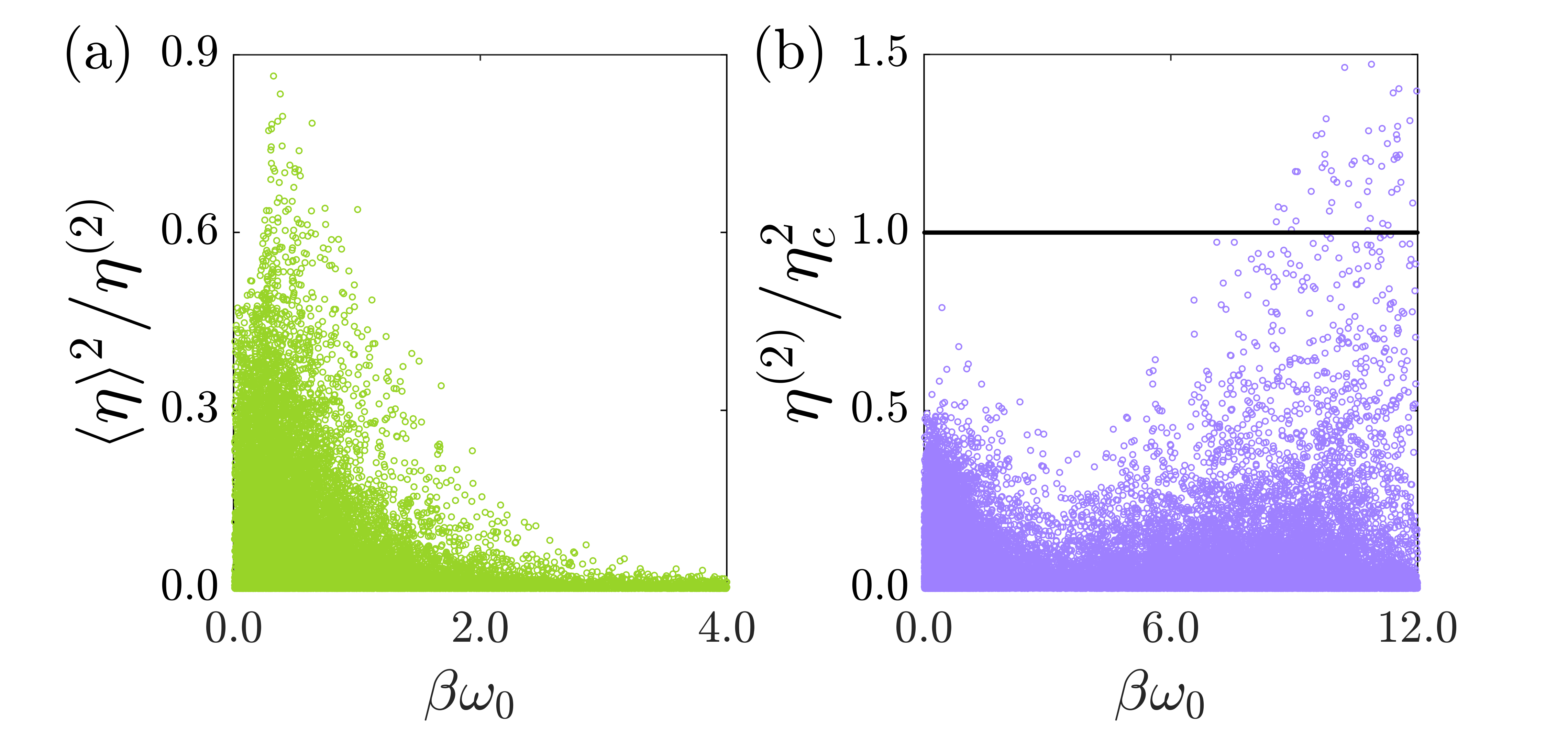
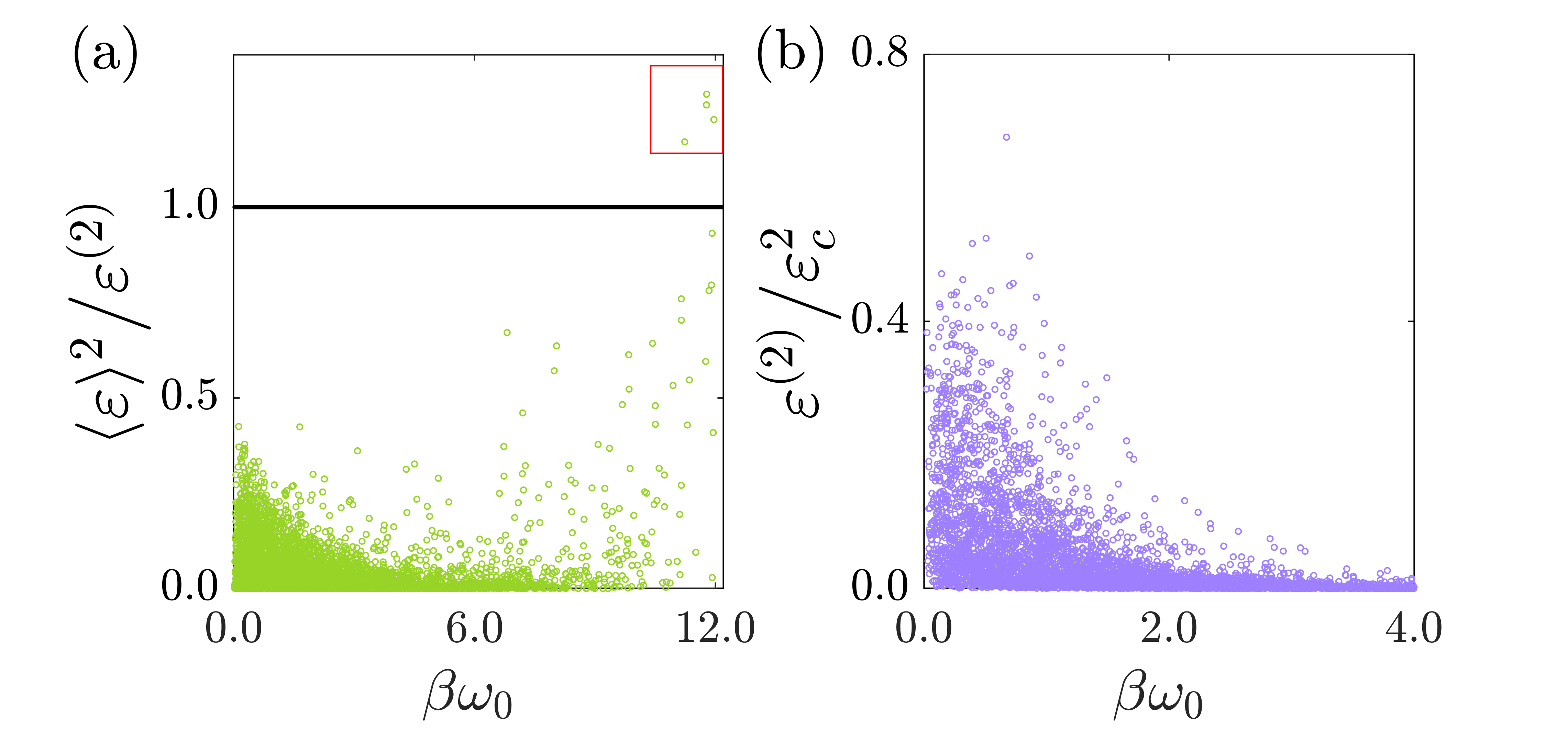
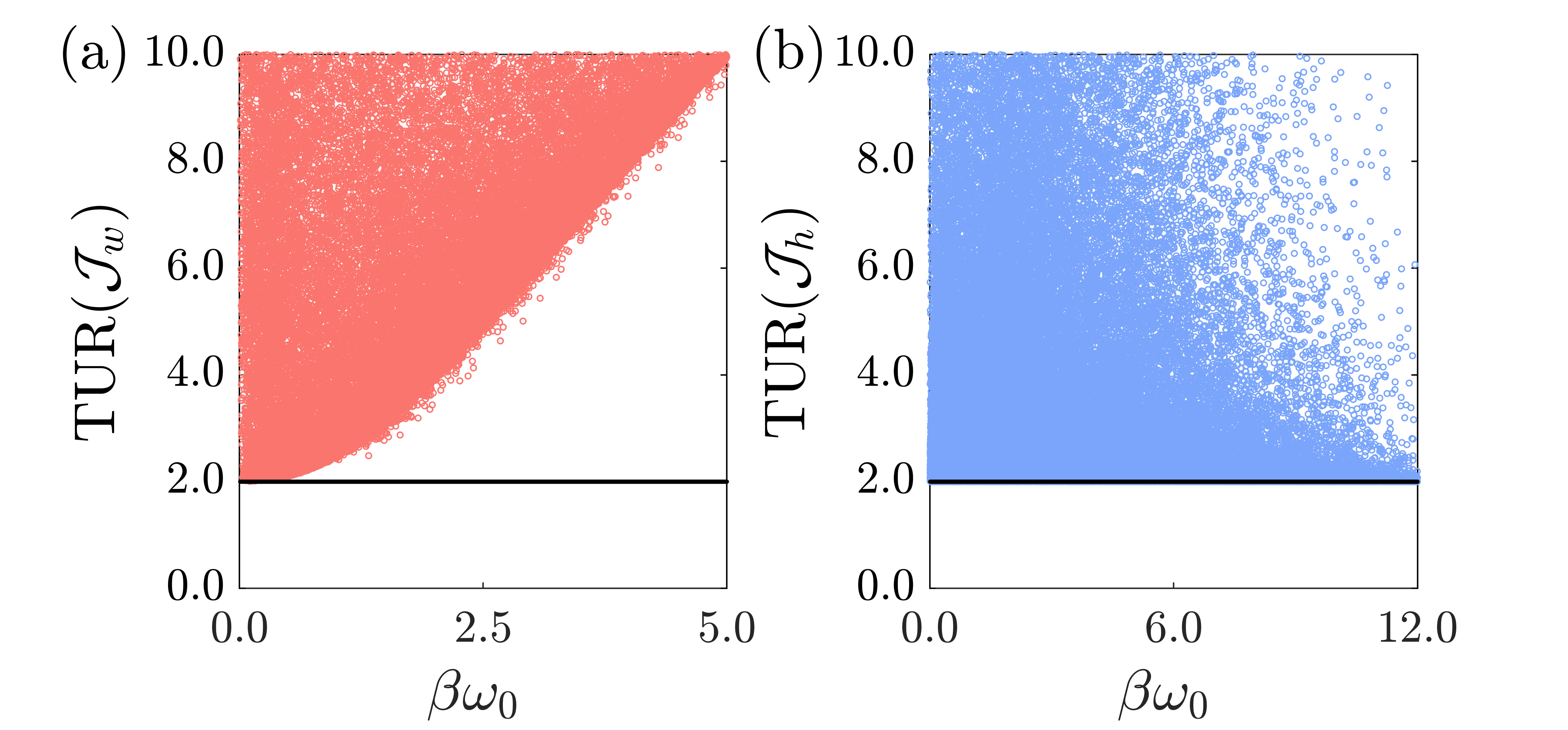
In the following, we present numerical results for N=5N\!=\!5 bosons confined in a harmonic trap. Starting from the single particle partition function Z1=csch(βω0/2)/2Z_{1}\!=\operatorname{csch}\big{(}\beta\hbar\omega_{0}/2\big{)}/2, we use the recursion relation given in Eq. (57) to calculate Z5Z_{5}. The various Onsager coefficients are computed numerically using Eqs. (64) to (66). We investigate bounds on the quantities η(2)\eta^{(2)} [defined in Eq. (43)] in the engine operational regime and ε(2)\varepsilon^{(2)} [defined in Eq. (48)] in the refrigerator operational regime. In Fig. 3 (a) we display the ratio η(2)/η2\eta^{(2)}/\langle\eta\rangle^{2}, which validates the existence of the lower bound, and in contrast to the autonomous continuous engine, the violation of the upper bound on η(2)\eta^{(2)} is observed in Fig. 3 (b). Furthermore, we observe the opposite trend in the refrigerator regime, i.e., the violation of the lower bound, and the existence of the upper bound, as shown in Fig. 4 (a) and (b), respectively. These observations precisely match our analytical predictions, and it is worth emphasizing that the central reason for the violation of these bounds in the linear response regime is due to the breakdown of the traditional FDR for work.

VI Summary

In this work, we utilized the Schwinger-Keldysh nonequilibrium Green’s function formalism to derive an analytical expression for the joint CGF for total work and heat from the hot reservoir in the quantum Otto cycle with an arbitrary many-body working medium. The derived CGF is valid up to the second order of the driving protocol λ(t)\lambda(t) and satisfies the heat engine fluctuation relation. This CGF is applicable to arbitrary perturbative protocols and interaction Hamiltonians. Furthermore, we developed a consistent linear response framework by focusing on the first and second cumulants of total work and heat in the limit of small driving amplitude and small temperature difference. Our analysis revealed the violation of the traditional FDR for the work current as a consequence of quantum non-adiabatic driving during the work strokes. However, for the heat current, the traditional FDR remains valid since the heat exchange stroke in the Otto cycle does not directly experience external driving. These findings have significant implications as they establish different universal bounds on fluctuations for the engine and refrigerator regimes. Specifically, in the engine regime, we observed that the ratio of output to input fluctuations is bounded from below, whereas in the refrigerator regime, the opposite trend is observed–the ratio of fluctuations is bounded from above. These results stand in stark contrast to the behavior observed for autonomous steady-state engines in earlier studies. Moreover, we found that the bounds on the ratio of fluctuations become similar for the two different families of machines only when the Otto cycle is driven in a quantum-adiabatic manner. This highlights the role of quantum effects in determining the bounds on fluctuations for thermal machines. Our study also established connections to the TURs for work and heat currents in the linear response regime, providing further insight into the thermodynamic behavior of the system. Future work will be directed toward analyzing the bounds beyond the linear response regime. It will be intriguing to extend the above analysis to other classes of quantum thermal machines and explore the implications of quantum effects on the performance and thermodynamic behavior of these systems.

ACKNOWLEDGMENTS

S.M. acknowledges financial support from the CSIR, India (File number: 09/936(0273)/2019-EMR-I). B.K.A. acknowledges the MATRICS grant MTR/2020/000472 from SERB, Government of India. B.K.A. also thanks the Shastri Indo-Canadian Institute for providing financial support for this research work in the form of a Shastri Institutional Collaborative Research Grant (SICRG).

Appendix A Joint CF on Keldysh contour:

In this Appendix, we present the details of obtaining the joint CF given in Eq. (3) in the main text. Recall that, the CF is the Fourier transform of the joint PD obtained by performing two-time measurements at the end-points of each stroke of the Otto cycle,

χ(γw,γh)=Tr[𝒰ee(iγwiγh)H(τ)𝒰ee(iγwβc)H(0)]×Tr[𝒰ceiγwH(0)𝒰ce(iγw+iγhβh)H(τ)]𝒵h1[H(τ)]𝒵c1[H(0)].\displaystyle\chi(\gamma_{w},\gamma_{h})={\mathrm{Tr}\big{[}{\cal U}_{\mathrm{e}}^{\dagger}e^{(i\gamma_{w}-i\gamma_{h})H(\tau)}{\cal U}_{\mathrm{e}}e^{(-i\gamma_{w}-\beta_{c})H(0)}\big{]}}\times{\mathrm{Tr}\big{[}{\cal U}_{\mathrm{c}}^{\dagger}e^{i\gamma_{w}H(0)}{\cal U}_{\mathrm{c}}e^{(-i\gamma_{w}+i\gamma_{h}-\beta_{h})H(\tau)}\big{]}}{{\cal Z}^{-1}_{h}[H(\tau)]}\,{{\cal Z}^{-1}_{c}[H(0)]}. (A1)

Here, the Hamiltonian of the working medium at any instant t[0,τ]t\in[0,\tau] is given by H(t)=H0+λ(t)H1H(t)\!=\!H_{0}+\lambda(t)H_{1}, where λ(0)=λ0\lambda(0)\!=\!\lambda_{0} and λ(τ)=λ1\lambda(\tau)\!=\!\lambda_{1}. In time-dependent perturbation theory, we express all the evolution operators in the interaction picture with respect to H0H_{0}. Here, we consider the first trace of Eq. (A1) only. A similar analysis applies to the second trace as well. For the sake of simplicity, we are dropping the e\mathrm{e} subscript from 𝒰e{\cal U}_{\mathrm{e}}. In the interaction picture. We obtain

𝒰I(t)=𝒯+exp[i0tλ(s)H1I(s)𝑑s],\displaystyle{\cal U}_{I}(t)={\cal T}_{+}\exp\Big{[}-\frac{i}{\hbar}\int_{0}^{t}\lambda(s)H_{1}^{I}(s)\,ds\Big{]}, (A2)
𝒰I(0)(t)=𝒯+exp[i0tλ0H1I(s)𝑑s],\displaystyle{\cal U}^{(0)}_{I}(t)={\cal T}_{+}\exp\Big{[}-\frac{i}{\hbar}\int_{0}^{t}\lambda_{0}H_{1}^{I}(s)\,ds\Big{]}, (A3)
𝒰I(τ)(t)=𝒯+exp[i0tλ1H1I(s)𝑑s],\displaystyle{\cal U}^{(\tau)}_{I}(t)={\cal T}_{+}\exp\Big{[}-\frac{i}{\hbar}\int_{0}^{t}\lambda_{1}H_{1}^{I}(s)\,ds\Big{]}, (A4)

where, the superscripts (0)(0) and (τ)(\tau) in Eqs. (A3) and (A4) indicate interaction picture evolution operator with fixed λ0\lambda_{0} and λ1\lambda_{1}, respectively. Here 𝒯+{\cal T}_{+} is the time-ordering operator which arranges the operators from left to right with decreasing time. Note that, H1I(s)=𝒰0(s)H1𝒰0(s)H_{1}^{I}(s)\!=\!{\cal U}_{0}^{\dagger}(s)\,H_{1}\,{\cal U}_{0}(s), where 𝒰0(t)=exp(iH0t/){\cal U}_{0}(t)\!=\!\exp{(\!-\!iH_{0}t/\hbar)} represents the free evolution operator. We express the first trace in Eq. (A1) as,

Tr\displaystyle\mathrm{Tr} [eiγwH(0)𝒰(τ)e(iγwiγh)H(τ)𝒰(τ)eβcH(0)]\displaystyle\Big{[}e^{-i\gamma_{w}H(0)}\,{\cal U}^{\dagger}(\tau)\,e^{(i\gamma_{w}-i\gamma_{h})H(\tau)}\,{\cal U}(\tau)\,e^{-\beta_{c}H(0)}\Big{]}
=\displaystyle= Tr[𝒰(0)(γw)𝒰(τ)𝒰(τ)(γw+γh)𝒰(τ)𝒰(0)(iβc)]\displaystyle\mathrm{Tr}\Big{[}{{\cal U}^{(0)}}^{\dagger}(-\hbar\gamma_{w})\,{\cal U}^{\dagger}(\tau)\,{{\cal U}^{(\tau)}}(-\hbar\gamma_{w}+\hbar\gamma_{h})\,{\cal U}(\tau)\,{{\cal U}^{(0)}}(-i\hbar\beta_{c})\Big{]}
=\displaystyle= Tr[𝒰I(0)(γw)𝒰0(γw)𝒰I(τ)𝒰0(τ)𝒰0(γw+γh)𝒰I(τ)(γw+γh)𝒰0(τ)𝒰I(τ)𝒰0(iβc)𝒰I(0)(iβc)]\displaystyle\mathrm{Tr}\Big{[}{{\cal U}_{I}^{(0)}}^{\dagger}(-\hbar\gamma_{w})\,{\cal U}_{0}^{\dagger}(-\hbar\gamma_{w})\,{\cal U}_{I}^{\dagger}(\tau)\,{\cal U}_{0}^{\dagger}(\tau)\,{\cal U}_{0}(-\hbar\gamma_{w}+\hbar\gamma_{h})\,{{\cal U}_{I}^{(\tau)}}(-\hbar\gamma_{w}+\hbar\gamma_{h})\,{\cal U}_{0}(\tau)\,{\cal U}_{I}(\tau)\,{\cal U}_{0}(-i\hbar\beta_{c})\,{{\cal U}_{I}^{(0)}}(-i\hbar\beta_{c})\Big{]}
=\displaystyle= Tr[𝒰0(iβc)𝒰0(γh)𝒰0(γh)𝒰I(0)(iβc)𝒰0(γh)𝒰0(γh)𝒰I(0)(γw)𝒰0(γh)\displaystyle\mathrm{Tr}\Big{[}{\cal U}_{0}(-i\hbar\beta_{c})\,{\cal U}_{0}(\hbar\gamma_{h})\,\overbrace{{\cal U}_{0}^{\dagger}(\hbar\gamma_{h})\,{\cal U}_{I}^{(0)}(-i\hbar\beta_{c})\,{\cal U}_{0}(\hbar\gamma_{h})}\,\underbrace{{\cal U}^{\dagger}_{0}(\hbar\gamma_{h})\,{{\cal U}_{I}^{(0)}}^{\dagger}(-\hbar\gamma_{w})\,{\cal U}_{0}(\hbar\gamma_{h})}\,
𝒰0(γw+γh)𝒰I(τ)𝒰0(γw+γh)𝒰0(τ)𝒰I(τ)(γw+γh)𝒰0(τ)𝒰I(τ)]\displaystyle\quad\quad\overbrace{{\cal U}_{0}^{\dagger}(-\hbar\gamma_{w}+\hbar\gamma_{h})\,{\cal U}_{I}^{\dagger}(\tau)\,{\cal U}_{0}(-\hbar\gamma_{w}+\hbar\gamma_{h})}\underbrace{{\cal U}_{0}^{\dagger}(\tau)\,{{\cal U}_{I}^{(\tau)}}(-\hbar\gamma_{w}+\hbar\gamma_{h})\,{\cal U}_{0}(\tau)}\,\overbrace{{\cal U}_{I}(\tau)}\Big{]}
=\displaystyle= 𝒯+eiγhγhiβcλ0H1I(s)𝑑s𝒯eiγw+γhγhλ0H1I(s)𝑑s𝒯eiτγw+γhγw+γhλ(s+γwγh)H1I(s)𝑑s\displaystyle\Big{\langle}{\cal T}_{+}e^{-\frac{i}{\hbar}\int_{\hbar\gamma_{h}}^{\hbar\gamma_{h}-i\hbar\beta_{c}}\lambda_{0}H_{1}^{I}(s)ds}\,{\cal T}_{-}e^{-\frac{i}{\hbar}\int_{-\hbar\gamma_{w}+\hbar\gamma_{h}}^{\hbar\gamma_{h}}\lambda_{0}H_{1}^{I}(s)ds}\,{\cal T}_{-}e^{-\frac{i}{\hbar}\int_{\tau-\hbar\gamma_{w}+\hbar\gamma_{h}}^{-\hbar\gamma_{w}+\hbar\gamma_{h}}\lambda(s+\gamma_{w}-\gamma_{h})H_{1}^{I}(s)ds}
𝒯+eiττγw+γhλ1H1I(s)𝑑s𝒯+ei0τλ(s)H1I(s)𝑑sβ~cTr[e(βciγh)H0]\displaystyle\quad\quad\,{\cal T}_{+}e^{-\frac{i}{\hbar}\int_{\tau}^{\tau-\hbar\gamma_{w}+\hbar\gamma_{h}}\lambda_{1}H_{1}^{I}(s)ds}\,{\cal T}_{+}e^{-\frac{i}{\hbar}\int_{0}^{\tau}\lambda(s)H_{1}^{I}(s)ds}\Big{\rangle}_{\widetilde{\beta}_{c}}\mathrm{Tr}\Big{[}e^{(-\beta_{c}-i\gamma_{h})H_{0}}\Big{]}
=\displaystyle= 𝒯ceicλC(s)H1I(s)𝑑sβ~cTr[e(βciγh)H0].\displaystyle\Big{\langle}{\cal T}_{c}\,e^{-\frac{i}{\hbar}\int_{c}\lambda_{C}(s)H_{1}^{I}(s)\,ds}\Big{\rangle}_{\widetilde{\beta}_{c}}\,\mathrm{Tr}\Big{[}e^{(-\beta_{c}-i\gamma_{h})H_{0}}\Big{]}. (A5)

In the last line, we map the real-time evolution onto a modified Keldysh contour CC [see Fig. 2 (a) in the main text] by introducing the contour-time ordered operator 𝒯C{\cal T}_{C} with contour-time dependent driving parameter λC(s)\lambda_{C}(s). Similarly, we can map the partition function 𝒵c[H(0)]{\cal Z}_{c}[H(0)] appearing in Eq. (A1) onto the same contour CC. For the partition function, we obtain

𝒵c[H(0)]\displaystyle{\cal Z}_{c}[H(0)] =Tr[eβcH(0)]=Tr[𝒰0(iβc)𝒰I(0)(iβc)]=Tr[𝒰0(iβc)𝒰0(γh)𝒰I(0)(iβc)𝒰0(γh)]\displaystyle=\mathrm{Tr}\Big{[}e^{-\beta_{c}H(0)}\Big{]}=\mathrm{Tr}\Big{[}\,{\cal U}_{0}(-i\hbar\beta_{c})\,{\cal U}_{I}^{(0)}(-i\hbar\beta_{c})\,\Big{]}=\mathrm{Tr}\Big{[}\,{\cal U}_{0}(-i\beta_{c})\,{\cal U}^{\dagger}_{0}(\hbar\gamma_{h})\,{\cal U}_{I}^{(0)}(-i\hbar\beta_{c})\,{\cal U}_{0}(\hbar\gamma_{h})\,\Big{]}
=𝒯ceiγhγhiβcλ0H1I(s)𝑑sβcTr[eβcH0],\displaystyle=\Big{\langle}{\cal T}_{c}\,e^{-\frac{i}{\hbar}\int_{\hbar\gamma_{h}}^{\hbar\gamma_{h}-i\hbar\beta_{c}}\lambda_{0}H_{1}^{I}(s)\,ds}\Big{\rangle}_{{\beta}_{c}}\,\mathrm{Tr}\big{[}e^{-\beta_{c}H_{0}}\big{]}, (A6)

where the contour-time dependent first term is mapped onto a Keldysh contour which runs only on the vertical line of Fig. 2 (a). The same prescription also applies for the second trace and the partition function 𝒵h[H(τ)]{\cal Z}_{h}[H(\tau)] in Eq. (A1), resulting in the second modified contour [see Fig. 2 (b)].

Appendix B Details of the calculation of joint CGF

In this Appendix, we will provide details of the derivation of Eq. (5). We will closely follow the prescription provided in Ref. Fei and Quan (2020). Here, we will demonstrate the series expansion for the first contour of the joint heat and work characteristic function:

χc(γw,γh)\displaystyle\chi_{c}(\gamma_{w},\gamma_{h}) 𝒯CeiCλC(s1)H1I(s1)𝑑s1β~c𝒯Ceiγhγhiβcλ0H1I(s1)𝑑s1βc\displaystyle\coloneqq\frac{\big{\langle}{\cal T}_{C}\,e^{-\frac{i}{\hbar}\int_{C}\!\lambda_{C}(s_{1})H_{1}^{I}(s_{1})ds_{1}}\big{\rangle}_{\widetilde{\beta}_{c}}}{\big{\langle}{\cal T}_{C}\,e^{-\frac{i}{\hbar}\int_{\hbar\gamma_{h}}^{\hbar\gamma_{h}\!-\!i\hbar\beta_{c}}\!\lambda_{0}H_{1}^{I}(s_{1})ds_{1}}\big{\rangle}_{{\beta}_{c}}}
=1+n=1[j=1nC𝑑sjλC(sj)ΘC(sjsj+1)(i)nH1I(s1)H1I(sn)β~c]1+n=1[j=1nγhγhiβc𝑑sjλC(sj)ΘC(sjsj+1)(i)nH1I(s1)H1I(sn)βc],\displaystyle=\frac{1+\displaystyle\sum_{n=1}^{\infty}\bigg{[}\prod_{j=1}^{n}\int_{C}ds_{j}\lambda_{C}(s_{j})\Theta_{C}(s_{j}\!-\!s_{j+1})\left(\!-\frac{i}{\hbar}\right)^{n}\big{\langle}H_{1}^{I}(s_{1})...H_{1}^{I}(s_{n})\big{\rangle}_{\widetilde{\beta}_{c}}\bigg{]}}{1+\displaystyle\sum_{n=1}^{\infty}\bigg{[}\prod_{j=1}^{n}\int_{\hbar\gamma_{h}}^{\hbar\gamma_{h}-i\hbar\beta_{c}}ds_{j}\lambda_{C}(s_{j})\Theta_{C}(s_{j}\!-\!s_{j+1})\left(\!-\frac{i}{\hbar}\right)^{n}\big{\langle}H_{1}^{I}(s_{1})...H_{1}^{I}(s_{n})\big{\rangle}_{{\beta}_{c}}\bigg{]}}, (B1)

where, the contour step function ΘC(sjsj+1)\Theta_{C}(s_{j}\!-\!s_{j+1}) is appearing because of the contour-time ordering. A more convenient way is to consider the expansion of the cumulant generating function ln[χc(γw,γh)]\ln[\chi_{c}(\gamma_{w},\gamma_{h})], where the series expansion is expressed in terms of nn-point connected correlation functions (cumulant correlation functions),

lnχc(γw,γh)=n=1[j=1nC𝑑𝐒jG~c(s1,,sn)j=1nγhγhiβc𝑑𝐒jGc(s1,,sn)],\displaystyle\ln\,\chi_{c}(\gamma_{w},\gamma_{h})=\sum_{n=1}^{\infty}\bigg{[}\prod_{j=1}^{n}\int_{C}d\mathbf{S}_{j}\widetilde{G}_{c}(s_{1},...,s_{n})-\prod_{j=1}^{n}\int_{\hbar\gamma_{h}}^{\hbar\gamma_{h}-i\hbar\beta_{c}}d\mathbf{S}_{j}{G}_{c}(s_{1},...,s_{n})\bigg{]}, (B2)

where, d𝐒j=dsjλC(sj)ΘC(sjsj+1)d\mathbf{S}_{j}=ds_{j}\lambda_{C}(s_{j})\Theta_{C}(s_{j}\!-\!s_{j+1}) and

G~c(s1,,sn)\displaystyle\widetilde{G}_{c}(s_{1},...,s_{n}) =(i)nH1I(s1)H1I(sn)β~c,\displaystyle=\left(\!-\frac{i}{\hbar}\right)^{n}\!\mathopen{\hbox{\set@color${\langle}$}\kern-1.94444pt\leavevmode\hbox{\set@color${\langle}$}}H_{1}^{I}(s_{1})...H_{1}^{I}(s_{n})\mathclose{\hbox{\set@color${\rangle}$}\kern-1.94444pt\leavevmode\hbox{\set@color${\rangle}$}}_{\widetilde{\beta}_{c}},
Gc(s1,,sn)\displaystyle{G}_{c}(s_{1},...,s_{n}) =(i)nH1I(s1)H1I(sn)βc.\displaystyle=\left(\!-\frac{i}{\hbar}\right)^{n}\!\mathopen{\hbox{\set@color${\langle}$}\kern-1.94444pt\leavevmode\hbox{\set@color${\langle}$}}H_{1}^{I}(s_{1})...H_{1}^{I}(s_{n})\mathclose{\hbox{\set@color${\rangle}$}\kern-1.94444pt\leavevmode\hbox{\set@color${\rangle}$}}_{{\beta}_{c}}. (B3)

Note that, .\mathopen{\hbox{\set@color${\langle}$}\kern-1.94444pt\leavevmode\hbox{\set@color${\langle}$}}.\mathclose{\hbox{\set@color${\rangle}$}\kern-1.94444pt\leavevmode\hbox{\set@color${\rangle}$}} represents cumulant correlation function [see Eq. (8) in the main text]. Crucially, the contour-time dependent driving parameter λC(s)\lambda_{C}(s) is piece-wise defined along the contour CC:

λ(s)={λ(s)Part 1:s[0,τ),λ1Part 2:s[τ,τγw+γh),λ(s+γwγh)Part 3:s[τγw+γh,γw+γh),λ0Part 4:s[γw+γh,γhiβc].\displaystyle\lambda(s)=\begin{cases}\lambda(s)&\mathrm{Part}\;1:\;s\in[0,\tau),\\ \lambda_{1}&\mathrm{Part}\;2:\;s\in[\tau,\tau\!-\!\hbar\gamma_{w}+\hbar\gamma_{h}),\\ \lambda(s+\hbar\gamma_{w}\!-\!\hbar\gamma_{h})&\mathrm{Part}\;3:\;s\in[\tau\!-\!\hbar\gamma_{w}+\hbar\gamma_{h},-\hbar\gamma_{w}+\hbar\gamma_{h}),\\ \lambda_{0}&\mathrm{Part}\;4:\;s\in[-\hbar\gamma_{w}+\hbar\gamma_{h},\hbar\gamma_{h}\!-\!i\hbar\beta_{c}].\end{cases} (B4)

In what follows, we will calculate the right-hand side of Eq. (B2) up to the second order of the driving parameter λ(s)\lambda(s). The contribution to the first order of λ(s)\lambda(s) is given by

i[γw(λ1λ0)γhλ1]H1β~cβcλ0[H1β~cH1βc].\displaystyle i\big{[}\gamma_{w}(\lambda_{1}\!-\!\lambda_{0})-\gamma_{h}\lambda_{1}\big{]}\langle H_{1}\rangle_{\widetilde{\beta}_{c}}-\beta_{c}\lambda_{0}\big{[}\langle H_{1}\rangle_{\widetilde{\beta}_{c}}\!-\!\langle H_{1}\rangle_{{\beta}_{c}}\big{]}. (B5)

Next, for the contribution to the second order in λ(s)\lambda(s) we have to calculate double integrals given by

C𝑑s1λC(s1)C𝑑s2λC(s2)ΘC(s1s2)G~c(s1,s2)γhγhiβc𝑑s1λC(s1)γhγhiβc𝑑s2λC(s2)ΘC(s1s2)Gc(s1,s2)\displaystyle\int_{C}\!\!ds_{1}\,\lambda_{C}(s_{1})\!\int_{C}\!\!ds_{2}\,\lambda_{C}(s_{2})\,\Theta_{C}(s_{1}\!-\!s_{2})\,\widetilde{G}_{c}(s_{1},s_{2})-\!\!\int_{\hbar\gamma_{h}}^{\hbar\gamma_{h}\!-\!i\hbar\beta_{c}}\!\!ds_{1}\,\lambda_{C}(s_{1})\!\int_{\hbar\gamma_{h}}^{\hbar\gamma_{h}\!-\!i\hbar\beta_{c}}\!\!ds_{2}\,\lambda_{C}(s_{2})\,\Theta_{C}(s_{1}\!-\!s_{2})\,G_{c}(s_{1},s_{2})
=\displaystyle= C𝑑s1λC(s1)C𝑑s2λC(s2)ΘC(s1s2)G~c>(s1s2)γhγhiβc𝑑s1λC(s1)γhγhiβc𝑑s2λC(s2)ΘC(s1s2)Gc>(s1s2).\displaystyle\int_{C}\!\!ds_{1}\,\lambda_{C}(s_{1})\!\!\int_{C}\!ds_{2}\,\lambda_{C}(s_{2})\,\Theta_{C}(s_{1}\!-\!s_{2})\,\widetilde{G}_{c}^{>}(s_{1}\!-\!s_{2})-\!\!\int_{\hbar\gamma_{h}}^{\hbar\gamma_{h}\!-\!i\hbar\beta_{c}}\!\!ds_{1}\,\lambda_{C}(s_{1})\!\!\int_{\hbar\gamma_{h}}^{\hbar\gamma_{h}\!-\!i\hbar\beta_{c}}\!\!ds_{2}\,\lambda_{C}(s_{2})\,\Theta_{C}(s_{1}\!-\!s_{2})\,G_{c}^{>}(s_{1}\!-\!s_{2}). (B6)

Note that the greater Green’s functions are introduced in Eq. (7) in the main text. Due to Eq. (B4), the double integral along the contour CC is expressed as a sum of double integrals of parts (i,j)(i,j), where i,j{1,2,3,4}i,j\in\{1,2,3,4\}. Importantly, once we take into account the contour step function Θ(s1s2)\Theta(s_{1}\!-\!s_{2}), only 10 out of the possible 16 terms survive in this sum:

(i,j)={(1,1),(2,1),(2,2),(3,1),(3,2),(3,3),(4,1),(4,2),(4,3),(4,4).\displaystyle(i,j)=\begin{cases}(1,1),\\ (2,1),\;(2,2),\\ (3,1),\;(3,2),\;(3,3),\\ (4,1),\;(4,2),\;(4,3),\;(4,4).\end{cases} (B7)

Bellow we show details of calculating a few of these double integrations:

1. For (i,j)=(4,1)(i,j)=(4,1)

dω2πγw+γhγhiβc𝑑s1λ0eiωs10τ𝑑s2λ(s2)eiωs2G~c>(ω)\displaystyle\int\frac{d\omega}{2\pi}\int_{-\!\hbar\gamma_{w}+\hbar\gamma_{h}}^{\hbar\gamma_{h}\!-\!i\hbar\beta_{c}}\!ds_{1}\,\lambda_{0}\,e^{-i\omega s_{1}}\int_{0}^{\tau}\!ds_{2}\,\lambda(s_{2})\,e^{i\omega s_{2}}\widetilde{G}_{c}^{>}(\omega)
=dω2πλ0eω(βc+iγh)G~c>(ω)iω0τ𝑑s2λ(s2)eiωs2dω2πλ0G~c>(ω)iωeiω(γwγh)0τ𝑑s2λ(s2)eiωs2\displaystyle=\int\frac{d\omega}{2\pi}\lambda_{0}\frac{e^{-\hbar\omega(\beta_{c}+i\gamma_{h})}\widetilde{G}_{c}^{>}(\omega)}{-i\omega}\int_{0}^{\tau}\!ds_{2}\,\lambda(s_{2})\,e^{i\omega s_{2}}-\int\frac{d\omega}{2\pi}\lambda_{0}\frac{\widetilde{G}_{c}^{>}(\omega)}{-i\omega}\,e^{i\hbar\omega(\gamma_{w}-\gamma_{h})}\int_{0}^{\tau}\!ds_{2}\,\lambda(s_{2})\,e^{i\omega s_{2}}
=dω2πλ0G~c>(ω)iω0τ𝑑s2λ(s2)eiωs2+dω2πλ0G~c>(ω)iωeiω(γwγh)0τ𝑑s2λ(s2)eiωs2\displaystyle=\int\frac{d\omega}{2\pi}\lambda_{0}\frac{\widetilde{G}_{c}^{>}(-\omega)}{-i\omega}\int_{0}^{\tau}\!ds_{2}\,\lambda(s_{2})\,e^{i\omega s_{2}}+\int\frac{d\omega}{2\pi}\lambda_{0}\frac{\widetilde{G}_{c}^{>}(\omega)}{i\omega}\,e^{i\hbar\omega(\gamma_{w}-\gamma_{h})}\int_{0}^{\tau}\!ds_{2}\,\lambda(s_{2})\,e^{i\omega s_{2}}
=dω2πG~c>(ω)iωλ00τ𝑑s2λ(s2)eiωs2+dω2πG~c>(ω)iωλ0eiω(γwγh)0τ𝑑s2λ(s2)eiωs2.\displaystyle=\int\frac{d\omega}{2\pi}\frac{\widetilde{G}_{c}^{>}(\omega)}{i\omega}\,\lambda_{0}\int_{0}^{\tau}\!ds_{2}\,\lambda(s_{2})\,e^{-i\omega s_{2}}+\int\frac{d\omega}{2\pi}\frac{\widetilde{G}_{c}^{>}(\omega)}{i\omega}\,\lambda_{0}\,e^{i\hbar\omega(\gamma_{w}-\gamma_{h})}\int_{0}^{\tau}\!ds_{2}\,\lambda(s_{2})\,e^{i\omega s_{2}}. (B8)

where to go from the second step to the third step we have used the KMS relation given in Eq. (12) in the main text.

2. For (i,j)=(4,2)(i,j)=(4,2)

dω2πγw+γhγhiβc𝑑s1λ0eiωs1ττγw+γh𝑑s2λ1eiωs2G~c>(ω)\displaystyle\int\frac{d\omega}{2\pi}\int_{-\!\hbar\gamma_{w}+\hbar\gamma_{h}}^{\hbar\gamma_{h}\!-\!i\hbar\beta_{c}}\!ds_{1}\,\lambda_{0}\,e^{-i\omega s_{1}}\int_{\tau}^{\tau\!-\!\hbar\gamma_{w}+\hbar\gamma_{h}}\!ds_{2}\,\lambda_{1}\,e^{i\omega s_{2}}\widetilde{G}_{c}^{>}(\omega)
=dω2πλ0λ1eω(βc+iγh)G~c>(ω)ω2(1eiω(γwγh))eiωτdω2πλ0λ1G~c>(ω)ω2(1eiω(γwγh))eiωτ\displaystyle=-\int\frac{d\omega}{2\pi}\lambda_{0}\lambda_{1}\frac{e^{-\hbar\omega(\beta_{c}+i\gamma_{h})}\widetilde{G}_{c}^{>}(\omega)}{\omega^{2}}\big{(}1-e^{-i\hbar\omega(\gamma_{w}-\gamma_{h})}\big{)}\,e^{i\omega\tau}-\int\frac{d\omega}{2\pi}\lambda_{0}\lambda_{1}\frac{\widetilde{G}_{c}^{>}(\omega)}{\omega^{2}}\big{(}1-e^{i\hbar\omega(\gamma_{w}-\gamma_{h})}\big{)}\,e^{i\omega\tau}
=dω2πλ0λ1G~c>(ω)ω2(1eiω(γwγh))eiωτdω2πλ0λ1G~c>(ω)ω2(1eiω(γwγh))eiωτ\displaystyle=-\int\frac{d\omega}{2\pi}\lambda_{0}\lambda_{1}\frac{\widetilde{G}_{c}^{>}(-\omega)}{\omega^{2}}\big{(}1-e^{-i\hbar\omega(\gamma_{w}-\gamma_{h})}\big{)}\,e^{i\omega\tau}-\int\frac{d\omega}{2\pi}\lambda_{0}\lambda_{1}\frac{\widetilde{G}_{c}^{>}(\omega)}{\omega^{2}}\big{(}1-e^{i\hbar\omega(\gamma_{w}-\gamma_{h})}\big{)}\,e^{i\omega\tau}
=dω2πG~c>(ω)ω2[2λ0λ1(1eiω(γwγh))cos(ωτ)],\displaystyle=\int\frac{d\omega}{2\pi}\frac{\widetilde{G}_{c}^{>}(\omega)}{\omega^{2}}\big{[}-{2\lambda_{0}\lambda_{1}}\big{(}1-e^{i\hbar\omega(\gamma_{w}-\gamma_{h})}\big{)}\,\cos{(\omega\tau)}\big{]}, (B9)

3. For (i,j)=(4,3)(i,j)=(4,3)

dω2πγw+γhγhiβc𝑑s1λ0eiωs1τγw+γhγw+γh𝑑s2λ(s2+γwγh)eiωs2G~c>(ω)\displaystyle\int\frac{d\omega}{2\pi}\int_{-\!\hbar\gamma_{w}+\hbar\gamma_{h}}^{\hbar\gamma_{h}\!-\!i\hbar\beta_{c}}\!ds_{1}\,\lambda_{0}\,e^{-i\omega s_{1}}\int_{\tau-\hbar\gamma_{w}+\hbar\gamma_{h}}^{-\hbar\gamma_{w}+\hbar\gamma_{h}}\!ds_{2}\,\lambda(s_{2}+\hbar\gamma_{w}-\hbar\gamma_{h})\,e^{i\omega s_{2}}\widetilde{G}_{c}^{>}(\omega)
=dω2πγw+γhγhiβc𝑑s1λ0eiωs10τ𝑑s2λ(s2)eiω(s2γw+γh)G~c>(ω)\displaystyle=-\int\frac{d\omega}{2\pi}\int_{-\!\hbar\gamma_{w}+\hbar\gamma_{h}}^{\hbar\gamma_{h}\!-\!i\hbar\beta_{c}}\!ds_{1}\,\lambda_{0}\,e^{-i\omega s_{1}}\int_{0}^{\tau}\!ds_{2}\,\lambda(s_{2})\,e^{i\omega(s_{2}-\hbar\gamma_{w}+\hbar\gamma_{h})}\widetilde{G}_{c}^{>}(\omega)
=dω2πG~c>(ω)iωλ0eiω(γwγh)0τ𝑑s2λ(s2)eiωs2dω2πG~c>(ω)iωλ00τ𝑑s2λ(s2)eiωs2.\displaystyle=-\int\frac{d\omega}{2\pi}\frac{\widetilde{G}_{c}^{>}(\omega)}{i\omega}\,\lambda_{0}\,e^{i\hbar\omega(\gamma_{w}-\gamma_{h})}\int_{0}^{\tau}\!ds_{2}\,\lambda(s_{2})\,e^{-i\omega s_{2}}-\int\frac{d\omega}{2\pi}\frac{\widetilde{G}_{c}^{>}(\omega)}{i\omega}\,\lambda_{0}\int_{0}^{\tau}\!ds_{2}\,\lambda(s_{2})\,e^{i\omega s_{2}}. (B10)

The intermediate steps are similar to the (4,1) case.

4. For (i,j)=(4,4)(i,j)=(4,4)

dω2πγw+γhγhiβc𝑑s1λ0eiωs1γw+γhs1𝑑s2λ0eiωs2G~c>(ω)dω2πγhγhiβc𝑑s1λ0eiωs1γhs1𝑑s2λ0eiωs2Gc>(ω)\displaystyle\int\frac{d\omega}{2\pi}\int_{-\!\hbar\gamma_{w}+\hbar\gamma_{h}}^{\hbar\gamma_{h}\!-\!i\hbar\beta_{c}}\!ds_{1}\,\lambda_{0}\,e^{-i\omega s_{1}}\int_{-\hbar\gamma_{w}+\hbar\gamma_{h}}^{s_{1}}\!ds_{2}\,\lambda_{0}\,e^{i\omega s_{2}}\widetilde{G}_{c}^{>}(\omega)-\int\frac{d\omega}{2\pi}\int_{\hbar\gamma_{h}}^{\hbar\gamma_{h}\!-\!i\hbar\beta_{c}}\!ds_{1}\,\lambda_{0}\,e^{-i\omega s_{1}}\int_{\hbar\gamma_{h}}^{s_{1}}\!ds_{2}\,\lambda_{0}\,e^{i\omega s_{2}}{G}_{c}^{>}(\omega)
=dω2πG~c>(ω)ω2λ02[iωγwβcω+1eβcωeiωγw]dω2πGc>(ω)ω2λ02[βcω+1eβcω]\displaystyle=\int\frac{d\omega}{2\pi}\frac{\widetilde{G}_{c}^{>}(\omega)}{\omega^{2}}\lambda_{0}^{2}\big{[}-i\hbar\omega\gamma_{w}-\beta_{c}\hbar\omega+1-e^{-\beta_{c}\hbar\omega}e^{-i\hbar\omega\gamma_{w}}\big{]}-\int\frac{d\omega}{2\pi}\frac{{G}_{c}^{>}(\omega)}{\omega^{2}}\lambda_{0}^{2}\big{[}-\beta_{c}\hbar\omega+1-e^{-\beta_{c}\omega}\big{]}
=dω2πλ02[G~c>(ω)ω2(iωγwβcω+1)eiω(γwγh)G~c>(ω)ω2]dω2πλ02[Gc>(ω)ω2(βcω+1)Gc>(ω)ω2]\displaystyle=\int\frac{d\omega}{2\pi}\lambda_{0}^{2}\Big{[}\frac{\widetilde{G}_{c}^{>}(\omega)}{\omega^{2}}\big{(}-i\hbar\omega\gamma_{w}-\beta_{c}\hbar\omega+1\big{)}-e^{-i\hbar\omega(\gamma_{w}-\gamma_{h})}\frac{\widetilde{G}_{c}^{>}(-\omega)}{\omega^{2}}\Big{]}-\int\frac{d\omega}{2\pi}\lambda_{0}^{2}\Big{[}\frac{{G}_{c}^{>}(\omega)}{\omega^{2}}\big{(}-\beta_{c}\hbar\omega+1)-\frac{{G}_{c}^{>}(-\omega)}{\omega^{2}}\Big{]}
=dω2πG~c>(ω)ω2λ02[iωγwβcω+1eiω(γwγh)]+dω2πGc>(ω)ωλ02βc.\displaystyle=\int\frac{d\omega}{2\pi}\frac{\widetilde{G}_{c}^{>}(\omega)}{\omega^{2}}\lambda_{0}^{2}\big{[}-i\hbar\omega\gamma_{w}-\beta_{c}\hbar\omega+1-e^{i\hbar\omega(\gamma_{w}-\gamma_{h})}\big{]}+\int\frac{d\omega}{2\pi}\frac{{G}_{c}^{>}(\omega)}{\omega}\lambda_{0}^{2}\beta_{c}\hbar. (B11)

Note that, the second term here is stemming from the canonical partition function 𝒵c[H(0)]{\cal Z}_{c}[H(0)] [second term in Eq. (B6)]. The rest of the terms in Eq. (B7) can be calculated analogously. Now, following Ref. Fei and Quan (2020), we will categorize the 10 non-zero terms given in Eq. (B7) in 6 groups:

  1. 1.

    {(2,2)}\{(2,2)\}:

    dω2πG~c>(ω)[λ12ω2(iω(γwγh)+1eiω(γwγh))].\displaystyle\int\frac{d\omega}{2\pi}\widetilde{G}_{c}^{>}(\omega)\Big{[}\frac{\lambda_{1}^{2}}{\omega^{2}}\big{(}i\hbar\omega(\gamma_{w}-\gamma_{h})+1-e^{i\hbar\omega(\gamma_{w}-\gamma_{h})}\big{)}\Big{]}. (B12)
  2. 2.

    {(1,1)+(3,1)+(3,3)}\{(1,1)+(3,1)+(3,3)\}

    dω2πG~c>(ω)(1eiω(γwγh))0τ𝑑s10τ𝑑s2λ(s1)λ(s2)eiω(s1s2).\displaystyle\int\frac{d\omega}{2\pi}\widetilde{G}_{c}^{>}(\omega)\,\Big{(}1-e^{i\hbar\omega(\gamma_{w}-\gamma_{h})}\Big{)}\int_{0}^{\tau}ds_{1}\int_{0}^{\tau}ds_{2}\,\lambda(s_{1})\lambda(s_{2})e^{i\omega(s_{1}-s_{2})}. (B13)
  3. 3.

    {(2,1)+(3,2)}\{(2,1)+(3,2)\}

    dω2πG~c>(ω)[2λ1ω(1eiω(γwγh))0τ𝑑sλ(s)sin[ω(τs)]].\displaystyle\int\frac{d\omega}{2\pi}\widetilde{G}_{c}^{>}(\omega)\Big{[}-\frac{2\lambda_{1}}{\omega}\Big{(}1-e^{i\hbar\omega(\gamma_{w}-\gamma_{h})}\Big{)}\int_{0}^{\tau}ds\,\lambda(s)\sin{[\omega(\tau-s)]}\Big{]}. (B14)
  4. 4.

    {(4,3)+(4,1)}\{(4,3)+(4,1)\}

    dω2πG~c>(ω)[2λ0ω(1eiω(γwγh))0τ𝑑sλ(s)sin(ωs)].\displaystyle\int\frac{d\omega}{2\pi}\widetilde{G}_{c}^{>}(\omega)\Big{[}-\frac{2\lambda_{0}}{\omega}\Big{(}1-e^{i\hbar\omega(\gamma_{w}-\gamma_{h})}\Big{)}\int_{0}^{\tau}ds\,\lambda(s)\sin{(\omega s)}\Big{]}. (B15)
  5. 5.

    {(4,2)}\{(4,2)\}

    dω2πG~c>(ω)[2λ0λ1ω2(1eiω(γwγh))cos(ωτ)].\displaystyle\int\frac{d\omega}{2\pi}{\widetilde{G}_{c}^{>}(\omega)}\Big{[}-\frac{2\lambda_{0}\lambda_{1}}{\omega^{2}}\Big{(}1-e^{i\hbar\omega(\gamma_{w}-\gamma_{h})}\Big{)}\,\cos{(\omega\tau)}\Big{]}. (B16)
  6. 6.

    {(4,4)}\{(4,4)\}

    dω2πG~c>(ω)[λ02ω2(iωγwβcω+1eiω(γwγh))]+dω2πGc>(ω)βcλ02ω.\displaystyle\int\frac{d\omega}{2\pi}{\widetilde{G}_{c}^{>}(\omega)}\Big{[}\frac{\lambda_{0}^{2}}{\omega^{2}}\Big{(}-i\hbar\omega\gamma_{w}-\beta_{c}\hbar\omega+1-e^{i\hbar\omega(\gamma_{w}-\gamma_{h})}\Big{)}\Big{]}+\int\frac{d\omega}{2\pi}{{G}_{c}^{>}(\omega)}\frac{\hbar\beta_{c}\lambda_{0}^{2}}{\omega}. (B17)

We further collect all the terms with (1eiω(γwγh))\big{(}1-e^{i\hbar\omega(\gamma_{w}-\gamma_{h})}\big{)}

dω2πG~c>(ω)1eiω(γwγh)ω2[λ12+λ022λ0λ1cos(ωτ)+ω20τds10τds2λ(s1)λ(s2)eiω(s1s2)\displaystyle\int\frac{d\omega}{2\pi}{\widetilde{G}_{c}^{>}(\omega)}\frac{1-e^{i\hbar\omega(\gamma_{w}-\gamma_{h})}}{\omega^{2}}\Big{[}\lambda_{1}^{2}+\lambda_{0}^{2}-2\lambda_{0}\lambda_{1}\cos{(\omega\tau)}+\omega^{2}\int_{0}^{\tau}ds_{1}\int_{0}^{\tau}ds_{2}\,\lambda(s_{1})\lambda(s_{2})e^{i\omega(s_{1}-s_{2})}
2ωλ10τdsλ(s)sin[ω(τs)]2ωλ00τdsλ(s)sin(ωs)]\displaystyle\quad\quad\quad-2\omega\lambda_{1}\int_{0}^{\tau}ds\,\lambda(s)\sin{[\omega(\tau-s)]}-2\omega\lambda_{0}\int_{0}^{\tau}ds\,\lambda(s)\sin{(\omega s)}\Big{]}
=dω2πG~c>(ω)1eiω(γwγh)ω2|λ1eiωτλ0iω0τ𝑑sλ(s)eiωs|2\displaystyle=\int\frac{d\omega}{2\pi}{\widetilde{G}_{c}^{>}(\omega)}\frac{1-e^{i\hbar\omega(\gamma_{w}-\gamma_{h})}}{\omega^{2}}\bigg{|}\lambda_{1}e^{i\omega\tau}-\lambda_{0}-i\omega\int_{0}^{\tau}ds\,\lambda(s)\,e^{i\omega s}\bigg{|}^{2}
=dω2πG~c>(ω)1eiω(γwγh)ω2|0τ𝑑sλ˙(s)eiωs|2\displaystyle=\int\frac{d\omega}{2\pi}{\widetilde{G}_{c}^{>}(\omega)}\frac{1-e^{i\hbar\omega(\gamma_{w}-\gamma_{h})}}{\omega^{2}}\bigg{|}\int_{0}^{\tau}ds\,\dot{\lambda}(s)\,e^{i\omega s}\bigg{|}^{2}
=dω2πG~c>(ω)1eiω(γwγh)ω2A(ω),\displaystyle=\int\frac{d\omega}{2\pi}{\widetilde{G}_{c}^{>}(\omega)}\frac{1-e^{i\hbar\omega(\gamma_{w}-\gamma_{h})}}{\omega^{2}}\,A(\omega), (B18)

where A(ω)=|0τ𝑑sλ˙(s)eiωs|2A(\omega)\!=\!\big{|}\int_{0}^{\tau}ds\,\dot{\lambda}(s)\,e^{i\omega s}\big{|}^{2} encapsulates information on the speed of the driving protocol λ(s)\lambda(s). Finally, summing all the terms given in Eqs. (B12) to (B17), we obtain

dω2πG~c>(ω)[1ω(iγw(λ12λ02)iγhλ12βcλ02)+1eiω(γwγh)ω2A(ω)]+dω2πGc>(ω)βcλ02ω.\displaystyle\int\frac{d\omega}{2\pi}{\widetilde{G}_{c}^{>}(\omega)}\bigg{[}\frac{1}{\omega}\Big{(}i\hbar\gamma_{w}(\lambda_{1}^{2}-\lambda_{0}^{2})-i\hbar\gamma_{h}\lambda_{1}^{2}-\hbar\beta_{c}\lambda_{0}^{2}\Big{)}+\frac{1-e^{i\hbar\omega(\gamma_{w}-\gamma_{h})}}{\omega^{2}}\,A(\omega)\bigg{]}+\int\frac{d\omega}{2\pi}{{G}_{c}^{>}(\omega)}\frac{\hbar\beta_{c}\lambda_{0}^{2}}{\omega}. (B19)

Therefore, the right-hand side of Eq. (B2) up to second order of driving parameter λ(s)\lambda(s) is given by

i(γw(λ1λ0)γhλ1)\displaystyle i\Big{(}\gamma_{w}(\lambda_{1}\!-\!\lambda_{0})-\gamma_{h}\lambda_{1}\Big{)} H1β~cβcλ0(H1β~cH1βc)+(iγw(λ12λ02)iγhλ12βcλ02)dω2πG~c>(ω)ω\displaystyle\langle H_{1}\rangle_{\widetilde{\beta}_{c}}-\beta_{c}\lambda_{0}\Big{(}\langle H_{1}\rangle_{\widetilde{\beta}_{c}}\!-\!\langle H_{1}\rangle_{{\beta}_{c}}\Big{)}+\Big{(}i\hbar\gamma_{w}(\lambda_{1}^{2}-\lambda_{0}^{2})-i\hbar\gamma_{h}\lambda_{1}^{2}-\hbar\beta_{c}\lambda_{0}^{2}\Big{)}\int\frac{d\omega}{2\pi}\frac{{\widetilde{G}_{c}^{>}(\omega)}}{\omega}
+βcλ02dω2πGc>(ω)ω+dω2πG~c>(ω)1eiω(γwγh)ω2A(ω).\displaystyle+\hbar\beta_{c}\lambda_{0}^{2}\int\frac{d\omega}{2\pi}\frac{{{G}_{c}^{>}(\omega)}}{\omega}+\int\frac{d\omega}{2\pi}{{\widetilde{G}_{c}^{>}(\omega)}}\frac{1-e^{i\hbar\omega(\gamma_{w}-\gamma_{h})}}{\omega^{2}}\,A(\omega). (B20)

It is essential to highlight that the contour CC corresponding to the first trace in Eq. (2) in the main text, contains all the contributions to the statistics of total work and input heat that are solely connected to the cold reservoir inverse temperature βc\beta_{c}. An analogous calculation can be done for the second contour CC^{\prime}, which captures all the contributions that are connected to the hot reservoir inverse temperature βh\beta_{h}.

Appendix C Proof for heat FDR

In this Appendix, we will demonstrate the proof for the heat FDR given by Eq. (32) in the main text. We start with Eq. (19) and take the limit of w=0\mathcal{F}_{w}\!=\!0 and q=0\mathcal{F}_{q}\!=\!0. This immediately hands over the following expression for heat-fluctuation

𝒥h2|w=0q=0\displaystyle\mathopen{\hbox{\set@color${\langle}$}\kern-1.94444pt\leavevmode\hbox{\set@color${\langle}$}}\mathcal{J}_{h}^{2}\mathclose{\hbox{\set@color${\rangle}$}\kern-1.94444pt\leavevmode\hbox{\set@color${\rangle}$}}\Big{|}_{\begin{subarray}{c}\mathcal{F}_{w}=0\\ \mathcal{F}_{q}=0\end{subarray}}\! =1τcyc[H02βc+H02βh+2λ1[H0H1βc+H0H1βh]+2λ12dωπGc(ω)+Gh(ω)ωβcλ0[H02H1βc\displaystyle=\frac{1}{\tau_{cyc}}\bigg{[}\mathopen{\hbox{\set@color${\langle}$}\kern-1.94444pt\leavevmode\hbox{\set@color${\langle}$}}H_{0}^{2}\mathclose{\hbox{\set@color${\rangle}$}\kern-1.94444pt\leavevmode\hbox{\set@color${\rangle}$}}_{\beta_{c}}\!+\mathopen{\hbox{\set@color${\langle}$}\kern-1.94444pt\leavevmode\hbox{\set@color${\langle}$}}H_{0}^{2}\mathclose{\hbox{\set@color${\rangle}$}\kern-1.94444pt\leavevmode\hbox{\set@color${\rangle}$}}_{\beta_{h}}\!+2\lambda_{1}\big{[}\mathopen{\hbox{\set@color${\langle}$}\kern-1.94444pt\leavevmode\hbox{\set@color${\langle}$}}H_{0}H_{1}\mathclose{\hbox{\set@color${\rangle}$}\kern-1.94444pt\leavevmode\hbox{\set@color${\rangle}$}}_{\beta_{c}}\!\!+\mathopen{\hbox{\set@color${\langle}$}\kern-1.94444pt\leavevmode\hbox{\set@color${\langle}$}}H_{0}H_{1}\mathclose{\hbox{\set@color${\rangle}$}\kern-1.94444pt\leavevmode\hbox{\set@color${\rangle}$}}_{\beta_{h}}\big{]}+2\hbar\lambda_{1}^{2}\!\!\int\!\frac{d\omega}{\pi}\frac{G_{c}^{{}^{\prime}}(\omega)+G_{h}^{{}^{\prime}}(\omega)}{\omega}\!-\!\beta_{c}\lambda_{0}\Big{[}\mathopen{\hbox{\set@color${\langle}$}\kern-1.94444pt\leavevmode\hbox{\set@color${\langle}$}}H_{0}^{2}H_{1}\mathclose{\hbox{\set@color${\rangle}$}\kern-1.94444pt\leavevmode\hbox{\set@color${\rangle}$}}_{\beta_{c}}
+λ0dω2πGc′′(ω)ω]βhλ1[H02H1βh+λ1dω2πGh′′(ω)ω]+2dω2πGc(ω)A(ω)ω+2dω2πA(ω)Gc>(ω)]w=0q=0\displaystyle\!\!+\hbar\lambda_{0}\!\!\int\!\frac{d\omega}{2\pi}\frac{G_{c}^{{}^{\prime\prime}}(\omega)}{\omega}\Big{]}\!-\!\beta_{h}\lambda_{1}\!\Big{[}\mathopen{\hbox{\set@color${\langle}$}\kern-1.94444pt\leavevmode\hbox{\set@color${\langle}$}}H_{0}^{2}H_{1}\mathclose{\hbox{\set@color${\rangle}$}\kern-1.94444pt\leavevmode\hbox{\set@color${\rangle}$}}_{\beta_{h}}\!\!+\hbar\lambda_{1}\!\!\int\!\frac{d\omega}{2\pi}\frac{G_{h}^{{}^{\prime\prime}}(\omega)}{\omega}\Big{]}\!+\!2\hbar\!\!\int\!\frac{d\omega}{2\pi}\frac{G^{{}^{\prime}}_{c}(\omega)A(\omega)}{\omega}+\hbar^{2}\!\!\int\!\frac{d\omega}{2\pi}{A(\omega)G_{c}^{>}(\omega)}\bigg{]}_{\begin{subarray}{c}\mathcal{F}_{w}=0\\ \mathcal{F}_{q}=0\end{subarray}}
=2τcyc{β[H0β+2λH1β+2λ2dω2πG>(ω)ω]βλ2β2[H1β+λdω2πG>(ω)ω]}\displaystyle=\frac{2}{\tau_{cyc}}\Big{\{}-\frac{\partial}{\partial\beta}\Big{[}\langle H_{0}\rangle_{\beta}+2\lambda\langle H_{1}\rangle_{\beta}+2\hbar\lambda^{2}\!\!\int\frac{d\omega}{2\pi}\frac{G^{>}(\omega)}{\omega}\Big{]}-\beta\lambda\frac{\partial^{2}}{\partial\beta^{2}}\Big{[}\langle H_{1}\rangle_{\beta}+\hbar\lambda\!\!\int\frac{d\omega}{2\pi}\frac{G^{>}(\omega)}{\omega}\Big{]}\Big{\}}
=2qq,\displaystyle=2\cdot\mathcal{L}_{qq}, (C1)

where we have used λ=λ0\lambda\!=\!\lambda_{0} and β=βc\beta\!=\!\beta_{c}, as adopted in the main text.

Appendix D Connection with the TURs

In this Appendix, we will provide proof for the thermodynamic uncertainty relations,

σ𝒥w2𝒥w22,σ𝒥h2𝒥h22,\displaystyle\langle\sigma\rangle\frac{\mathopen{\hbox{\set@color${\langle}$}\kern-1.94444pt\leavevmode\hbox{\set@color${\langle}$}}\mathcal{J}_{w}^{2}\mathclose{\hbox{\set@color${\rangle}$}\kern-1.94444pt\leavevmode\hbox{\set@color${\rangle}$}}}{\langle\mathcal{J}_{w}\rangle^{2}}\geq 2,\quad\langle\sigma\rangle\frac{\mathopen{\hbox{\set@color${\langle}$}\kern-1.94444pt\leavevmode\hbox{\set@color${\langle}$}}\mathcal{J}_{h}^{2}\mathclose{\hbox{\set@color${\rangle}$}\kern-1.94444pt\leavevmode\hbox{\set@color${\rangle}$}}}{\langle\mathcal{J}_{h}\rangle^{2}}\geq 2, (D1)

where the entropy production rate σ=w𝒥w+q𝒥h\sigma\!=\!{\cal F}_{w}\langle\mathcal{J}_{w}\rangle+{\cal F}_{q}\langle\mathcal{J}_{h}\rangle. Using Eqs. (27) and (37) we show that

σ𝒥w2𝒥w2\displaystyle\langle\sigma\rangle\frac{\mathopen{\hbox{\set@color${\langle}$}\kern-1.94444pt\leavevmode\hbox{\set@color${\langle}$}}\mathcal{J}_{w}^{2}\mathclose{\hbox{\set@color${\rangle}$}\kern-1.94444pt\leavevmode\hbox{\set@color${\rangle}$}}}{\langle\mathcal{J}_{w}\rangle^{2}} σ2ww𝒥w2\displaystyle\geq\langle\sigma\rangle\frac{2\cdot{\cal L}_{ww}}{\langle\mathcal{J}_{w}\rangle^{2}}
=(w𝒥w+q𝒥h)2ww𝒥w2\displaystyle=\big{(}{\cal F}_{w}\langle\mathcal{J}_{w}\rangle+{\cal F}_{q}\langle\mathcal{J}_{h}\rangle\big{)}\frac{2{\cal L}_{ww}}{\langle\mathcal{J}_{w}\rangle^{2}}
=2(ww2w2+2wwwqwq+wwqqq2)1𝒥w2\displaystyle=2\Big{(}{\cal L}_{ww}^{2}{\cal F}_{w}^{2}+2{\cal L}_{ww}{\cal L}_{wq}{\cal F}_{w}{\cal F}_{q}+{\cal L}_{ww}{\cal L}_{qq}{\cal F}_{q}^{2}\Big{)}\frac{1}{\langle\mathcal{J}_{w}\rangle^{2}}
=2(𝒥w2+[wwqqwq2])1𝒥w2\displaystyle=2\Big{(}\langle\mathcal{J}_{w}\rangle^{2}+\big{[}{\cal L}_{ww}{\cal L}_{qq}-{\cal L}_{wq}^{2}\big{]}\Big{)}\frac{1}{\langle\mathcal{J}_{w}\rangle^{2}}
=2+2det||𝒥w22.\displaystyle=2+\frac{2\cdot\mathrm{det}|{\cal L}|}{\langle\mathcal{J}_{w}\rangle^{2}}\geq 2. (D2)

The proof of the TUR corresponding to 𝒥h\mathcal{J}_{h} follows analogously. In Fig. 5 we display the TURs for work and heat currents for the trapped boson model considered in the main text.

Refer to caption
Figure 5: Thermodynamic Uncertainty Relations: TUR(𝒥i)=σ𝒥i2/𝒥i2\mathrm{TUR}(\mathcal{J}_{i})\!=\!\langle\sigma\rangle\mathopen{\hbox{\set@color${\langle}$}\kern-1.94444pt\leavevmode\hbox{\set@color${\langle}$}}\mathcal{J}_{i}^{2}\mathclose{\hbox{\set@color${\rangle}$}\kern-1.94444pt\leavevmode\hbox{\set@color${\rangle}$}}/\langle\mathcal{J}_{i}\rangle^{2}, where (a) i=wi\!=\!w, and (b) i=hi\!=\!h. These results correspond to the example presented in the main text, i.e., N=5 bosons trapped in a harmonic potential. Parameters chosen from uniform distributions: β[0, 4]\beta\in[0,\,4], ω0[0, 3]\omega_{0}\in[0,\,3], Δβ[0, 0.3β]\Delta\beta\in[0,\,0.3\beta], λ[0, 0.3]\lambda\in[0,\,0.3], and Δλ[0, 0.1]\Delta\lambda\in[0,\,0.1]. Simulations were done over one million points.

Appendix E Proof for 𝜼𝒄𝟐𝓕𝒘𝟐𝓛𝒘𝒘𝜷𝟐𝓛𝒒𝒒𝜼𝟐\bm{\eta_{c}^{2}\geq\frac{{\cal F}_{w}^{2}\mathcal{L}_{ww}}{\beta^{2}{\cal L}_{qq}}\geq\langle\eta\rangle^{2}}

In this Appendix, we will prove the inequalities stated in Eq. (42) in the main text step by step,

ηc2w2wwβ2qqη2.\displaystyle\eta_{c}^{2}\geq\frac{{\cal F}_{w}^{2}{\cal L}_{ww}}{\beta^{2}{\cal L}_{qq}}\geq\langle\eta\rangle^{2}. (E1)

Let us first consider the first inequality. We will consider a modified version: ηc2β2qqwww20\eta_{c}^{2}\beta^{2}\mathcal{L}_{qq}\!-\!\mathcal{L}_{ww}\mathcal{F}_{w}^{2}\geq 0. By using the fact that ηc=Δβ/β=q/β\eta_{c}\!=\!\Delta\beta/\beta\!=\!\mathcal{F}_{q}/\beta, we observe

ηc2β2qqwww2=\displaystyle\eta_{c}^{2}\beta^{2}\mathcal{L}_{qq}\!-\!\mathcal{L}_{ww}\mathcal{F}_{w}^{2}= qqq2www2\displaystyle\mathcal{L}_{qq}\mathcal{F}_{q}^{2}\!-\!\mathcal{L}_{ww}\mathcal{F}_{w}^{2}
=\displaystyle= qqq2+wqwqwqwqwww2\displaystyle\mathcal{L}_{qq}\mathcal{F}_{q}^{2}+\mathcal{L}_{wq}\mathcal{F}_{w}\mathcal{F}_{q}\!-\!\mathcal{L}_{wq}\mathcal{F}_{w}\mathcal{F}_{q}\!-\!\mathcal{L}_{ww}\mathcal{F}_{w}^{2}
=\displaystyle= q𝒥hw𝒥w\displaystyle\mathcal{F}_{q}\langle\mathcal{J}_{h}\rangle\!-\!\mathcal{F}_{w}\langle\mathcal{J}_{w}\rangle
=\displaystyle= q𝒥h[1+ηηc]\displaystyle\mathcal{F}_{q}\langle\mathcal{J}_{h}\rangle\Big{[}1+\frac{\langle\eta\rangle}{\eta_{c}}\Big{]}
\displaystyle\geq 0.\displaystyle 0. (E2)

In the above steps, we used the engine condition: 𝒥w<0\langle\mathcal{J}_{w}\rangle\!<\!0, and 𝒥h>0\langle\mathcal{J}_{h}\rangle\!>\!0. Next, let’s move on to the second inequality. Our strategy will be to consider a modified version of the second inequality: ww𝒥w2qq𝒥h20\mathcal{L}_{ww}\langle\mathcal{J}_{w}\rangle^{2}\!-\!\mathcal{L}_{qq}\langle\mathcal{J}_{h}\rangle^{2}\!\geq\!0. We observe

ww𝒥w2qq𝒥h2\displaystyle\mathcal{L}_{ww}\langle\mathcal{J}_{w}\rangle^{2}\!-\!\mathcal{L}_{qq}\langle\mathcal{J}_{h}\rangle^{2} =(wwqqwq2)[qqq2www2]\displaystyle=\big{(}\mathcal{L}_{ww}\mathcal{L}_{qq}\!-\!\mathcal{L}_{wq}^{2}\big{)}\Big{[}\mathcal{L}_{qq}\mathcal{F}_{q}^{2}\!-\!\mathcal{L}_{ww}\mathcal{F}_{w}^{2}\Big{]}
=det||[q𝒥hw𝒥w]\displaystyle=\mathrm{det}|\mathcal{L}|\Big{[}\mathcal{F}_{q}\langle\mathcal{J}_{h}\rangle\!-\!\mathcal{F}_{w}\langle\mathcal{J}_{w}\rangle\Big{]}
=det||q𝒥h[1+ηηc]\displaystyle=\mathrm{det}|\mathcal{L}|\,\mathcal{F}_{q}\langle\mathcal{J}_{h}\rangle\Big{[}1+\frac{\langle\eta\rangle}{\eta_{c}}\Big{]}
0.\displaystyle\geq 0. (E3)

It is important to note that, the two ingredients required for this proof are-

  1. 1.

    The positive semi-definiteness of the Onsager matrix, which implies that det||0\mathrm{det}|\mathcal{L}|\!\geq\!0, and

  2. 2.

    The characterization of engine operational regime by 𝒥w<0\langle\mathcal{J}_{w}\rangle\!<\!0 and 𝒥h>0\langle\mathcal{J}_{h}\rangle\!>\!0.

Appendix F Calculation of CGF for heat from the cold reservoir

The CF for qcq_{c} is obtained by setting γh=γw=γc\gamma_{h}\!=\!\gamma_{w}\!=\!-\gamma_{c} in Eq. (2). The new counting variable γc\gamma_{c} corresponds to the stochastic variable (wqh)(-w-q_{h}),

χ(γc)=𝑑w𝑑qhP(w,qh)eiγc(wqh).\displaystyle\chi(\gamma_{c})=\int\!\!\!\int d{w}\,d{q_{h}}\,P({w},{q_{h}})\,e^{i\gamma_{c}{(-w-q_{h})}}. (F1)

Interestingly, under the perfect thermalization condition with respect to heat reservoirs, the first law of thermodynamics holds even in the stochastic level, i.e., qc=wqhq_{c}=-w-q_{h}. This is rigorously proven in Appendix A of our previous work Mohanta et al. (2023). As a result, the CF in Eq. (F1) correctly provides the statistics of the exchanged heat qcq_{c} with respect to the cold reservoir. Finally, setting γh=γw=γc\gamma_{h}\!=\!\gamma_{w}\!=\!-\gamma_{c} in Eq. (5), we obtain the CGF for qcq_{c},

ln\displaystyle\ln χ(γc)=iγcλ0[H1β~hH1β~c]iγcλ02dω2πG~h>(ω)G~c>(ω)ωβcλ0[H1β~cH1βc+λ0dω2πG~c>(ω)Gc>(ω)ω]\displaystyle\chi(\gamma_{c})=-i\gamma_{c}\lambda_{0}\big{[}\langle H_{1}\rangle_{\widetilde{\beta}_{h}}\!\!-\!\langle H_{1}\rangle_{\widetilde{\beta}_{c}}\big{]}\!-\!i\gamma_{c}\hbar\lambda_{0}^{2}\!\!\int\!\frac{d\omega}{2\pi}\frac{\widetilde{G}_{h}^{>}(\omega)\!-\!\widetilde{G}_{c}^{>}(\omega)}{\omega}\!-\!\beta_{c}\lambda_{0}\Big{[}\langle H_{1}\rangle_{\widetilde{\beta}_{c}}\!\!-\!\langle H_{1}\rangle_{\beta_{c}}+\hbar\lambda_{0}\!\!\int\!\frac{d\omega}{2\pi}\frac{\widetilde{G}_{c}^{>}(\omega)\!-\!{G}_{c}^{>}(\omega)}{\omega}\Big{]}
βhλ1[H1β~hH1βh+λ1dω2πG~h>(ω)Gh>(ω)ω]+dω2π1eiωγcω2A(ω)G~h>(ω)+lneiγcH0βc+lneiγcH0βh.\displaystyle\!-\!\beta_{h}\lambda_{1}\Big{[}\langle H_{1}\rangle_{\widetilde{\beta}_{h}}\!\!-\!\langle H_{1}\rangle_{\beta_{h}}+\hbar\lambda_{1}\!\!\int\!\frac{d\omega}{2\pi}\frac{\widetilde{G}_{h}^{>}(\omega)\!-\!{G}_{h}^{>}(\omega)}{\omega}\Big{]}+\int\!\frac{d\omega}{2\pi}\frac{1\!-\!e^{-i\hbar\omega\gamma_{c}}}{\omega^{2}}{A}(\omega)\widetilde{G}_{h}^{>}(\omega)+\ln\langle e^{i\gamma_{c}H_{0}}\rangle_{\beta_{c}}+\ln\langle e^{-i\gamma_{c}H_{0}}\rangle_{\beta_{h}}. (F2)

A crucial point to note here is that now the shifted inverse temperatures become β~c=βciγc\widetilde{\beta}_{c}\!=\!\beta_{c}\!-\!i\gamma_{c} and β~h=βh+iγc\widetilde{\beta}_{h}\!=\!{\beta}_{h}+i\gamma_{c}, and consequently, G~h>(w)\widetilde{G}_{h}^{>}(w) and G~c>(w)\widetilde{G}_{c}^{>}(w) are redefined accordingly.

Appendix G Proof for 𝜺𝒄𝟐𝜷𝟐𝓛𝒒𝒒𝓕𝒘𝟐𝓛𝒘𝒘𝜺𝟐\bm{\varepsilon_{c}^{2}\geq\frac{\beta^{2}{\cal L}_{qq}}{{\cal F}_{w}^{2}{\cal L}_{ww}}\geq\langle\varepsilon\rangle^{2}}

In this Appendix, we will demonstrate the proof for the inequalities in Eq. (50) in the main text,

εc2β2qqw2wwε2.\displaystyle\varepsilon_{c}^{2}\geq\frac{\beta^{2}{\cal L}_{qq}}{{\cal F}_{w}^{2}{\cal L}_{ww}}\geq\langle\varepsilon\rangle^{2}. (G1)

To prove the first inequality, we start with the modified version of the first inequality www2β2qq/εc20\mathcal{L}_{ww}\mathcal{F}_{w}^{2}\!-\!\beta^{2}\mathcal{L}_{qq}/\varepsilon_{c}^{2}\geq 0:

www2β2qq/εc2=\displaystyle\mathcal{L}_{ww}\mathcal{F}_{w}^{2}\!-\!\beta^{2}\mathcal{L}_{qq}/\varepsilon_{c}^{2}= www2qqq2\displaystyle\mathcal{L}_{ww}\mathcal{F}_{w}^{2}\!-\!\mathcal{L}_{qq}\mathcal{F}_{q}^{2}
=\displaystyle= w𝒥wq𝒥h\displaystyle\mathcal{F}_{w}\langle\mathcal{J}_{w}\rangle\!-\!\mathcal{F}_{q}\langle\mathcal{J}_{h}\rangle
\displaystyle\approx w𝒥w+q𝒥c\displaystyle\mathcal{F}_{w}\langle\mathcal{J}_{w}\rangle+\mathcal{F}_{q}\langle\mathcal{J}_{c}\rangle
=\displaystyle= w𝒥w[1+εεc]\displaystyle\mathcal{F}_{w}\langle\mathcal{J}_{w}\rangle\Big{[}1+\frac{\langle\varepsilon\rangle}{\varepsilon_{c}}\Big{]}
\displaystyle\geq 0.\displaystyle 0. (G2)

Here, we have used the refrigerator condition: 𝒥c>0\langle\mathcal{J}_{c}\rangle\!>\!0, and 𝒥w>0\langle\mathcal{J}_{w}\rangle\!>\!0. To prove the second inequality, we start with the modified version of the second inequality as follows:

qq𝒥h2ww𝒥w2\displaystyle\mathcal{L}_{qq}\langle\mathcal{J}_{h}\rangle^{2}\!-\!\mathcal{L}_{ww}\langle\mathcal{J}_{w}\rangle^{2} =(wwqqwq2)[www2qqq2]\displaystyle=\big{(}\mathcal{L}_{ww}\mathcal{L}_{qq}\!-\!\mathcal{L}_{wq}^{2}\big{)}\Big{[}\mathcal{L}_{ww}\mathcal{F}_{w}^{2}\!-\!\mathcal{L}_{qq}\mathcal{F}_{q}^{2}\Big{]}
=det||[w𝒥w+q𝒥c]\displaystyle=\mathrm{det}|\mathcal{L}|\Big{[}\mathcal{F}_{w}\langle\mathcal{J}_{w}\rangle+\mathcal{F}_{q}\langle\mathcal{J}_{c}\rangle\Big{]}
=det||w𝒥w[1+εεc]\displaystyle=\mathrm{det}|\mathcal{L}|\,\mathcal{F}_{w}\langle\mathcal{J}_{w}\rangle\Big{[}1+\frac{\langle\varepsilon\rangle}{\varepsilon_{c}}\Big{]}
0.\displaystyle\geq 0. (G3)

In this case, the two ingredients required for this proof are-

  1. 1.

    The positive semi-definiteness of the Onsager matrix, which implies that det||0\mathrm{det}|\mathcal{L}|\!\geq\!0, and

  2. 2.

    The characterization of refrigerator operational regime by 𝒥c>0\langle\mathcal{J}_{c}\rangle\!>\!0 and 𝒥w>0\langle\mathcal{J}_{w}\rangle\!>\!0.

References