¹¹institutetext: Hong Kong University of Science and Technology
¹¹email: {jganad,golin}@cse.ust.hk

Fully Dynamic $k$ -Center in Low Dimensions via Approximate Furthest Neighbors

Jinxiang Gan Mordecai Jay Golin

Abstract

Let $P$ be a set of points in some metric space. The approximate furthest neighbor problem is, given a second point set $C,$ to find a point $p\in P$ that is a $(1+\epsilon)$ approximate furthest neighbor from $C.$

The dynamic version is to maintain $P,$ over insertions and deletions of points, in a way that permits efficiently solving the approximate furthest neighbor problem for the current $P.$

We provide the first algorithm for solving this problem in metric spaces with finite doubling dimension. Our algorithm is built on top of the navigating net data-structure.

An immediate application is two new algorithms for solving the dynamic $k$ -center problem. The first dynamically maintains $(2+\epsilon)$ approximate $k$ -centers in general metric spaces with bounded doubling dimension and the second maintains $(1+\epsilon)$ approximate Euclidean $k$ -centers. Both these dynamic algorithms work by starting with a known corresponding static algorithm for solving approximate $k$ -center, and replacing the static exact furthest neighbor subroutine used by that algorithm with our new dynamic approximate furthest neighbor one.

Unlike previous algorithms for dynamic $k$ -center with those same approximation ratios, our new ones do not require knowing $k$ or $\epsilon$ in advance. In the Euclidean case, our algorithm also seems to be the first deterministic solution.

Keywords:

PTAS, Dynamic Algorithms,

k

-center, Furthest Neighbor.

1 Introduction

The main technical result of this paper is an efficient procedure for calculating approximate furthest neighbors from a dynamically changing point set $P.$ This procedure, in turn, will lead to the development of two new simple algorithms for maintaining approximate $k$ -centers in dynamically changing point sets.

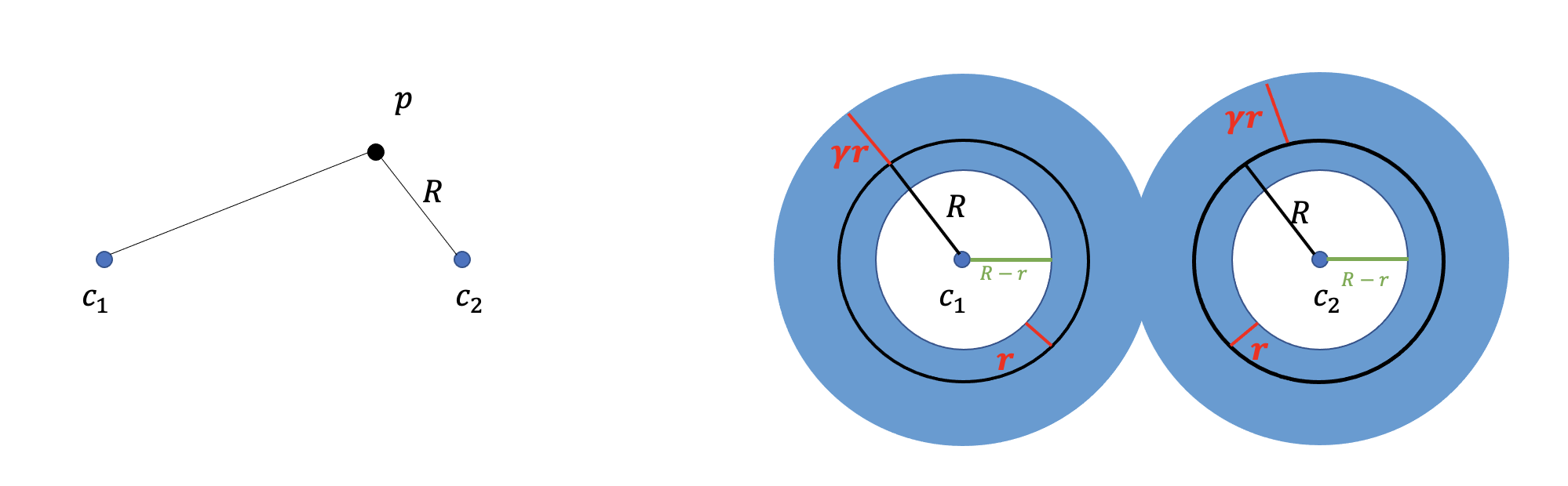
Let $B(c,r)$ denote the ball centered at $c$ with radius $r$ . The $k$ -center problem is to find a minimum radius $r^{*}$ and associated $C$ such that the union of balls $\bigcup_{c\in C}B(c,r^{*})$ contains all of the points in $P.$

In the arbitrary metric space version of the problem, the centers are restricted to be points in $P.$ In the Euclidean $k$ -center problem $(\mathcal{X},d)=\left(\mathbb{R}^{D},\ell_{2}\right)$ with $D\geq 1$ and $C$ may be any set of $k$ points in $\mathbb{R}^{D}.$ The Euclidean $1$ -center problem is also known as the minimum enclosing ball (MEB) problem.

An $\rho$ -approximation algorithm would find a set of centers $C^{\prime},$ $|C^{\prime}|\leq k,$ and radius $r^{\prime}$ in polynomial time such that $\bigcup_{c\in C^{\prime}}B(c,r^{\prime})$ contains all of the points in $P$ and $r^{\prime}\leq\rho r^{*}$ . The $k$ -center problem is known to be NP-hard to approximate with a factor smaller than 2 for arbitrary metric spaces[HN79], and with a factor smaller than $\sqrt{3}$ for Euclidean spaces [FG88].

Static algorithms

There do exist two 2-approximation algorithms in [Gon85, HS85] for the $k$ center problem on an arbitrary metric space; the best-known approximation factor for Euclidean $k$ -center remains 2 even for two-dimensional space when $k$ is part of the input (see [FG88]). There are better results for the special case of the Euclidean $k$ -center for fixed $k$ , $k=1$ or $2$ (e.g., see [BHPI02, BC03, AS10, KA15, KS20]). There are also PTASs [BHPI02, BC03, KS20] for the Euclidean $k$ center when $k$ and $D$ are constants.

Dynamic algorithms

In many practical applications, the data set $P$ is not static but changes dynamically over time, e.g, a new point may be inserted to or deleted from $P$ at each step. $C$ and $r$ then need to be recomputed at selected query times. If only insertions are permitted, the problem is incremental; if both insertions and deletions are permitted, the problem is fully dynamic.

The running time of such dynamic algorithms are often split into the time required for an update (to register a change in the storing data structure) and the time required for a query (to solve the problem on the current dataset). In dynamic algorithms, we require both update and query time to be nearly logarithmic or constant. The static versions take linear time.

Some known results on these problems are listed in Table 1. As is standard, many of them are stated in terms of the aspect ratio of point set $P$ . Let $d_{max}=\sup\{d(x,y):x,y\in P\text{ and }x\neq y\}$ and $d_{min}=\inf\{d(x,y):x,y\in P\text{ and }x\neq y\}$ . The aspect ratio $\Delta$ of $P$ is $\Delta=\frac{d_{max}}{d_{min}}$ .

Arbitrary Metric Space $(\mathcal{X},d)$
Author	Approx.	Dimensions	Update Time	Query Time	Fixed
Chan et al. [CGS18]	$2+\epsilon$	High	O( $k^{2}\frac{\log\Delta}{\epsilon}$ ) (avg.)	$O(k)$	$k,\epsilon$
Goranci et al. [GHL⁺21]	$2+\epsilon$	Low	$O((2/\epsilon)^{O(dim(\mathcal{X}))}\log\Delta\log\log\Delta\cdot\ln\epsilon^{-1})$	$O(\log\Delta+k)$	$\epsilon$
Bateni et al. [BEJM21]	$2+\epsilon$	High	$O(\frac{\log\Delta\log n}{\epsilon}(k+\log n)$ )(avg.)	$O(k)$	$k,\epsilon$
This paper	$2+\epsilon$	Low	$O\left(2^{O(dim(\mathcal{X}))}\log\Delta\log\log\Delta\right)$	$O(k^{2}(\log\Delta+(1/\epsilon)^{O(dim(\mathcal{X})}))$

Euclidean Space $(\mathbb{R}^{D},\ell_{2})$
Author	Approx.	Dimensions	Update Time	Query Time	Fixed
Chan [Cha09]	$1+\epsilon$	Low	$O((\frac{1}{\epsilon})^{D}k^{O(1)}\log n)$ (avg)	$O(\epsilon^{-D}k\log k\log n+(\frac{k}{\epsilon})^{O(k^{1-1/D})})$	$k,\epsilon$
Schmidt and Sohler [SS19]	$16$	Low	$O((2\sqrt{d}+1)^{d}\log^{2}\Delta\log n)$ (avg.)	$O((2\sqrt{d}+1)^{d}(\log\Delta+\log n))$
Schmidt and Sohler [SS19]	$O(f\cdot D)$	High	$O(D^{2}\log^{2}n\log\Delta n^{1/f})$ (avg.)	$O(f\cdot D\cdot\log n\log\Delta)$	$f$
(*) Bateni et al. [BEJM21]	$f(\sqrt{8}+\epsilon)$	High	$O(\frac{\log\delta^{-1}\log\Delta}{\epsilon}Dn^{1/f^{2}+o(1)})$		$\epsilon,f$
This paper	$1+\epsilon$	Low	$O\left(2^{O(D)}\log\Delta\log\log\Delta\right)$	$O(D\cdot k(\log\Delta+(1/\epsilon)^{O(D)})2^{k\log k/\epsilon})$

Table 1: Previous results on approximate dynamic

k

-centers. More information on the model used by each is in the text. Note that all algorithms listed provide correct results except for Schmidt and Sohler [SS19], which maintains

O(f\cdot D)

with probability

1-1/n

, and Bateni et al. [BEJM21], which maintains a

f(\sqrt{8}+\epsilon)

solution with probability

1-\delta

. [BEJM21] also combines the updates and queries.

The algorithms listed in the table work under slightly different models. More explicitly:

1.

For arbitrary metric spaces, both [GHL⁺21] and the current paper assume that the metric space has a bounded doubling dimension $dim(\mathcal{X})$ (see Definition 2).
2.

In “Low dimension”, update time may be exponential in $D$ ; in “High dimension” it may not.
3.

The “fixed” column denotes parameter(s) that must be fixed in advance when initializing the corresponding data structure, e.g., $k$ and/or $\epsilon.$ In addition, in both [SS19, BEJM21] for high dimensional space, $f\geqslant 1$ is a constant selected in advance that appears in both the approximation factor and running time.

The data structure used in the current paper is the navigating nets from [KL04]. It does not require knowing $k$ or $\epsilon$ in advance but instead supports them as parameters to the query.
4.

In [Cha09], (avg) denotes that the update time is in expectation (it is a randomized algorithm).
5.

Schmidt and Sohler [SS19] answers the slightly different membership query. Given $p$ , it returns the cluster containing $p.$ In low dimension, the running time of their algorithm is expected and amortized.

Our contributions and techniques

Our main results are two algorithms for solving the dynamic approximate $k$ -center problem in, respectively, arbitrary metric spaces with a finite doubling dimension and in Euclidean space.

1.

Our first new algorithm is for any metric space with finite doubling dimension:

Theorem 1.1

Let $(\mathcal{X},d)$ be a metric space with a finite doubling dimension $D$ . Let $P\subset X$ be a dynamically changing set of points. We can maintain $P$ in $O(2^{O(D)}\log\Delta\log\log\Delta)$ time per point insertion and deletion so as to support $(2+\epsilon)$ approximate $k$ -center queries in $O(k^{2}(\log\Delta+(1/\epsilon)^{O(D)}))$ time.

Compared with previous results (see table 1), our data structure does not require knowing $\epsilon$ or $k$ in advance, while the construction of the previous data structure depends on $k$ or $\epsilon$ as basic knowledge.
2.

Our second new algorithm is for the Euclidean $k$ -center problem:

Theorem 1.2

Let $P\subset\mathbb{R}^{D}$ be a dynamically changing set of points. We can maintain $P$ in $O(2^{O(D)}\log\Delta\log\log\Delta)$ time per point insertion and deletion so as to support $(1+\epsilon)$ approximate $k$ -center queries in $O(D\cdot k(\log\Delta+(1/\epsilon)^{O(D)})2^{k\log k/\epsilon})$ time.

This algorithm seems to be the first deterministic dynamic solution for the Euclidean $k$ -center problem. Chan [Cha09] presents a randomized dynamic algorithm while they do not find a way to derandomize it.

The motivation for our new approach was the observation that many previous results e.g., [BC03, BHPI02, Cha09, Gon85, KS20], on static $k$ -center, work by iteratively searching the furthest neighbor in $P$ from a changing set of points $C.$

Consider a set of $n$ points $P$ in some metric space $({\mathcal{X}},d).$ A nearest neighbor in $P$ to a query point $q,$ is a point $p\in P$ satisfying $d(p,q)=\min_{p^{\prime}\in P}d(p^{\prime},q)=d(P,q).$ A $(1+\epsilon)$ approximate nearest neighbor to $q$ is a point $p\in P$ satisfying $d(p,q)\leq(1+\epsilon)d(P,q).$

Similarly, a furthest neighbor to a query point $q$ is a $p$ satisfying $d(p,q)=\max_{p^{\prime}\in P}d(p^{\prime},q)$ . A $(1+\epsilon)$ approximate furthest neighbor to $q$ is a point $p\in P$ satisfying $\max_{p^{\prime}\in P}d(p^{\prime},q)\leq(1+\epsilon)d(p,q).$

There exist efficient algorithms for maintaining a dynamic point set $P$ (under insertions and deletions) that, given query point $q$ , quickly permit calculating approximate nearest [KL04] and furthest [Bes96, PSSS15, Cha16] neighbors to $q.$

A $(1+\epsilon)$ approximate nearest neighbor to a query set $C$ , is a point $p\in P$ satisfying $d(p,C)\leq(1+\epsilon)d(P,C)$ . Because “nearest neighbor” is decomposable, i.e., $d(P,C)=\min_{q\in C}d(P,q),$ [KL04] also permits efficiently calculating an approximate nearest neighbor to set $C$ from a dynamically changing $P.$

An approximate furthest neighbor to a query set $C$ is similarly defined as a point $p\in P$ satisfying $\max_{p^{\prime}\in P}d(p^{\prime},C)\leq(1+\epsilon)d(p,C).$ Our main new technical result is Theorem 2.1, which permits efficiently calculating an approximate furthest neighbor to query set $C$ from a dynamically changing $P.$ We note that, unlike nearest neighbor, furthest neighbor is not a decomposable problem and such a procedure does not seem to have previously known.

This technical result permits the creation of new algorithms for solving the dynamic $k$ -center problem in low dimensions.

2 Searching for a $(1+\epsilon)$ -Approximate Furthest Point in a Dynamically Changing Point Set

Let $(\mathcal{X},d)$ denote a fixed metric space.

Definition 1

Let $C,P\subset\mathcal{X}$ be finite sets of points and $q\in\mathcal{X}$ . Set

d({C},q)=d(q,C)=\min_{q^{\prime}\in{C}}d(q^{\prime},q)\quad\mbox{and}\quad d({C},P)=\min_{p\in P}d(C,p).

$p\in P$ is a furthest neighbor in $P$ to $q$ if $d(q,p)=\max_{p^{\prime}\in P}d(q,p^{\prime}).$

$p\in P$ is a furthest neighbor in $P$ to set $C$ if $d(C,p)=\max_{p^{\prime}\in P}d(C,p^{\prime}).$

$p\in P$ is a $(1+\epsilon)$ -approximate furthest neighbor in $P$ to $q$ if

\max_{p^{\prime}\in P}d(q,p^{\prime})\leq(1+\epsilon)d(q,p).

$p\in P$ is a $(1+\epsilon)$ -approximate furthest neighbor in $P$ to $C$ if

\max_{p^{\prime}\in P}d(C,p^{\prime})\leq(1+\epsilon)d(C,p).

$\mbox{FN}(P,q)$ and $\mbox{AFN}(P,q,\epsilon)$ will, respectively, denote procedures returning a furthest neighbor and a $(1+\epsilon)$ -approximate furthest neighbor to $q$ in $P.$

$\mbox{FN}(P,C)$ and $\mbox{AFN}(P,C,\epsilon)$ will, respectively, denote procedures returning a furthest neighbor and $(1+\epsilon)$ -approximate furthest neighbor to $C$ in $P.$

Our algorithm assumes that $\mathcal{X}$ has finite doubling dimension.

Definition 2 (Doubling Dimensions)

The doubling dimension of a metric space $(\mathcal{X},d)$ is the minimum value $\dim(\mathcal{X})$ such that any ball $B(x,r)$ in $(\mathcal{X},d)$ can be covered by $2^{\dim(\mathcal{X})}$ balls of radius $r/2$ .

It is known that the doubling dimension of the Euclidean space $(R^{D},\ell_{2})$ is $\Theta(D)$ [H⁺01].

Now let $(\mathcal{X},d)$ be a metric space with a finite doubling dimension and $P\subset\mathcal{X}$ be a finite set of points. Recall that $d_{max}=\sup\{d(x,y):x,y\in P\}\quad\mbox{and}\quad d_{min}=\inf\{d(x,y):x,y\in P,\ x\neq y\}.$ and The aspect ratio $\Delta$ of $P$ is $\Delta=\frac{d_{max}}{d_{min}}$ .

Our main technical theorem (proven below in Section 2.2) is:

Theorem 2.1

Let $(\mathcal{X},d)$ be a metric space with finite doubling dimension and $P\subset\mathcal{X}$ be a point set stored by a navigating net data structure [KL04]. Let $C\subset\mathcal{X}$ be another point set. Then, we can find a $(1+\epsilon)$ -approximate furthest point among $P$ to $C$ in $O\left(\mathcal{|C|}(\log\Delta+(1/\epsilon)^{O(\dim(\mathcal{X}))})\right)$ time, where $\Delta$ is the aspect ratio of set $P$ .

The navigating net data structure [KL04] is described in more detail below.

2.1 Navigating Nets [KL04]

Navigating nets are very well-known structures for dynamically maintaining points in a metric space with finite doubling dimension, in a way that permits approximate nearness queries. To the best of our knowledge they have not been previously used for approximate “furthest point from set” queries.

To describe the algorithm, we first need to quickly review some basic known facts about navigating nets. The following lemma is critical to our analysis.

Lemma 1

[KL04] Let $(\mathcal{X},d)$ be a metric space and $Y\subseteq\mathcal{X}$ . If the aspect ratio of the metric induced on $Y$ is at most $\Delta$ and $\Delta\geqslant 2$ , then $|Y|\leqslant\Delta^{O(\dim(\mathcal{X}))}$ .

We next introduce some notation from [KL04]:

Definition 3 ( $r$ -net)

[KL04] Let $(\mathcal{X},d)$ be a metric space. For a given parameter $r>0$ , a subset $Y\subseteq\mathcal{X}$ is an $r$ -net of $P$ if it satisfies:

(1)

For every $x,y\in Y$ , $d(x,y)\geqslant r$ ;
(2)

$\forall x\in P$ , there exists at least one $y\in Y$ such that $x\in B(y,r)$ .

We now start the description of the navigating net data structure. Set $\Gamma=\{2^{i}:i\in\mathbb{Z}\}$ . Each $r\in\Gamma$ is called a scale. For every $r\in\Gamma$ , $Y_{r}$ will denote an $r$ -net of $Y_{r/2}$ . The base case is that for every scale $r\leqslant d_{min}$ , $Y_{r}=P.$

Let $\gamma\geqslant 4$ be some fixed constant. For each scale $r$ and each $y\in Y_{r}$ , the data structure stores the set of points

L_{y,r}=\{z\in Y_{r/2}:d(z,y)\leqslant\gamma\cdot r\}.

(1)

$L_{y,r}$ is called the scale $r$ navigation list of $y$ .

Let $r_{max}\in\Gamma$ denote the smallest $r$ satisfying $|Y_{r}|=1$ and $r_{min}\in\Gamma$ denote the largest $r$ satisfying $L_{y,r}=\{y\}$ for every $y\in Y_{r}$ . Scales $r\in[r_{min},r_{max}]$ are called non-trivial scales; all other scales are called trivial. Since $r_{max}=\Theta(d_{max})$ and $r_{min}=\Theta(d_{min})$ , the number of non-trivial scales is $O\left(\log_{2}\frac{r_{max}}{r_{min}}\right)=O(\log_{2}\Delta).$

Finally, we need a few more basic properties of navigating nets:

Lemma 2

[KL04](Lemma 2.1 and 2.2) For each scale $r$ , we have:

(1)

$\forall y\in Y_{r}$ , $|L_{y,r}|=O(2^{O(\dim(\mathcal{X}))}).$
(2)

$\forall z\in P$ , $d(z,Y_{r})<2r$ ;
(3)

$\forall x,y\in Y_{r}$ , $d(x,y)\geqslant r$ .

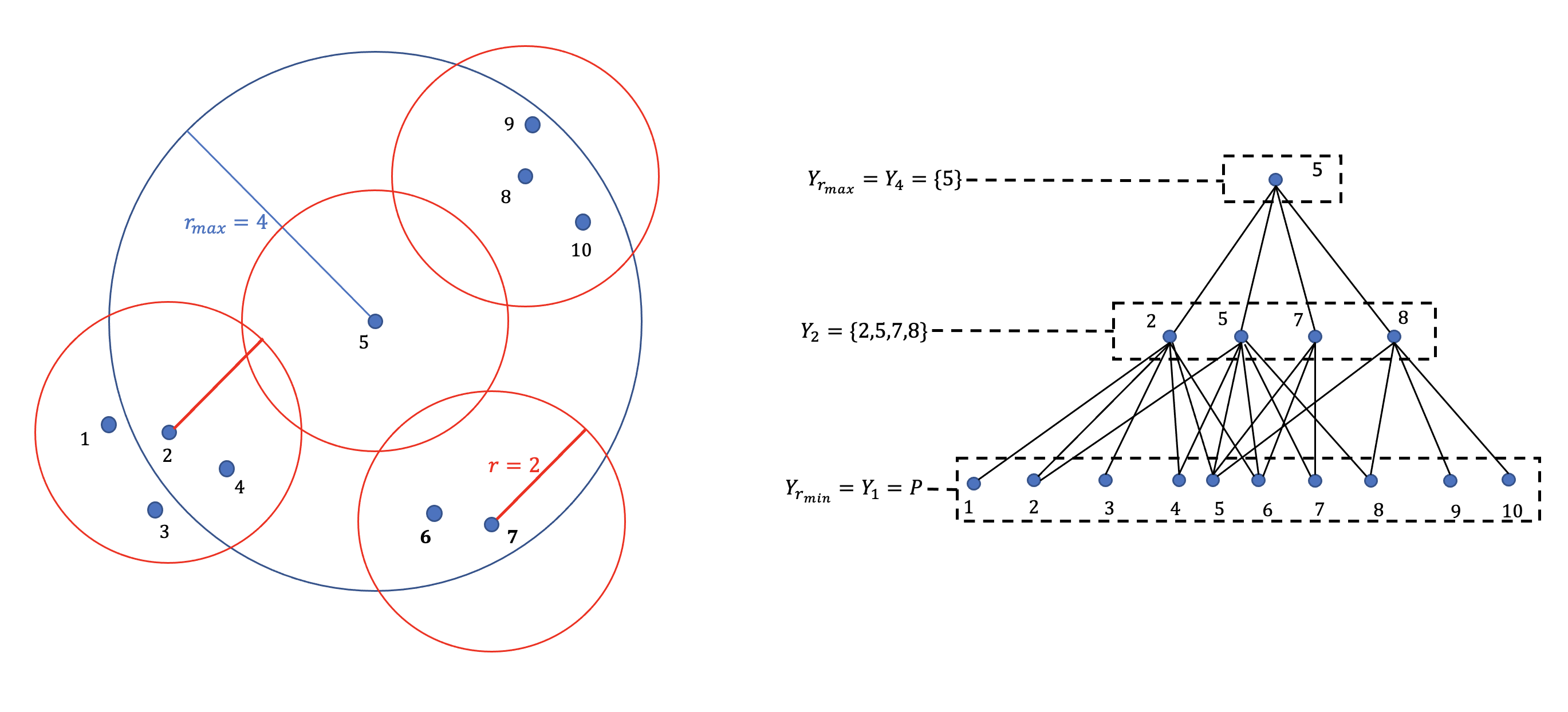
We provide an example (Figure 3) of navigating nets in the Appendix. Navigating nets were originally designed to solve dynamic approximate nearest neighbor queries and are useful because they can be quickly updated.

Theorem 2.2

([KL04]) Navigating nets use $O(2^{O(\dim(\mathcal{X}))}\cdot n)$ words. The data structure can be updated with an insertion of a point to $P$ or a deletion of a point in $P$ in time $(2^{O(\dim(\mathcal{X}))}\log\Delta\log\log\Delta)$ ¹¹1Note: Although the update time of the navigating net depends on $O(\log\Delta)$ , it does not explicitly maintain the value of $\Delta.$ Instead it dynamically maintains the values $r_{max}=\Theta(d_{max})$ and $r_{min}=\Theta(d_{min})$ . The update time depends on the number of non-trivial scales $\log\frac{r_{max}}{r_{min}}=\Theta(\log\Delta)$ , but without actually knowing $\Delta.$ . This includes $(2^{O(\dim(\mathcal{X}))}\log\Delta)$ distance computations.

2.2 The Approximate Furthest Neighbor Algorithm $\mbox{AFN}(P,C,\epsilon$ )

Algorithm 1 Approximate Furthest Neighbor:

\mbox{AFN}(P,C,\epsilon)

Input: A navigating net for set $P\subset\mathcal{X}$ , set $C\subset\mathcal{X}$ and a constant $\epsilon>0$ .
Output: A $(1+\epsilon)$ -approximate furthest neighbor among $P$ to $C$

1:Set

r=r_{max}

and

Z_{r}=Y_{r_{max}}

;

2:while

r>\max\{\frac{1}{2}(\epsilon\cdot\max_{z\in Z_{r}}d(z,C)),r_{min}

} do

3: set

Z_{r/2}=\bigcup_{z\in Z_{r}}\{y\in L_{z,r}:d(y,C)\geqslant\max_{z\in Z_{r}}d(z,C)-r\}

;

4: set

r=r/2

5:Return

z\in Z_{r}

satisfying

d(z,C)

is maximal.

$\mbox{AFN}(P,C,\epsilon)$ is given in Algorithm 1. Figure 1 provides some geometric intuition. $\mbox{AFN}(P,C,\epsilon)$ requires that $P$ be stored in a navigating net and the following definitions:

Definition 4 (The sets $Z_{r}$ )

•

$Z_{r_{max}}=Y_{r_{max}}$ , where $|Y_{r_{max}}|=1$ ;
•

If $Z_{r}$ is defined, $Z_{r/2}=\bigcup_{z\in Z_{r}}\{y\in L_{z,r}:d(y,C)\geqslant\max_{z\in Z_{r}}d(z,C)-r\}$ .

Note that, by induction, $Z_{r}\subseteq Y_{r}.$

Refer to caption — Figure 1: Illustration of line 3 of Algorithm 1. $C=\{c_{1},c_{2}\}$ . Let $p\in Z_{r}$ be the furthest point in $Z_{r}$ to $C$ and set $R=\max_{z\in Z_{r}}d(z,C)$ (in fig. 1, $R=d(c_{2},p)).$ , $Z_{r}\subseteq B(c_{1},R)\cup B(c_{2},R)$ . If $z\in B(c_{i},R)$ and $y\in L_{z,r}$ then $y\in B(c_{i},R+\gamma r).$ Next note that if $y\in Z_{r/2}$ then $y\in L_{z,r}$ for some $z\in Z_{r}$ and for each $i,$ $d(y,c_{i})\geq d(y,C)\geq R-r.$ This is illustrated in the right figure; $y$ must be in one of the two blue annulus $B(c_{i},R+\gamma r)\setminus B(c_{i},R-r)$ ( $i=1,2).$ Thus $Z_{r/2}$ is contained in the union of the annulus.

We now prove that $\mbox{AFN}(P,C,\epsilon)$ returns a $(1+\epsilon)$ -approximate furthest point among $P$ to $C$ . We start by showing that, for every scale $r,$ the furthest point to $C$ is close to $Z_{r}.$

Lemma 3

Let $a^{*}$ be the furthest point to $C$ in $P$ . Then, every set $Z_{r}$ as defined in Definition 4, contains a point $z_{r}$ satisfying $d(z_{r},a^{*})\leqslant 2r$

Proof

The proof is illustrated in Figure 2. It works by downward induction on $r$ . In the base case $r=r_{max}$ and $Z_{r_{max}}=Y_{r_{max}}$ , thus $d(a^{*},Z_{r_{max}})\leqslant 2r$ .

For the inductive step, we assume that $Z_{r}$ satisfies the induction hypothesis, i.e, $Z_{r}$ contains a point $z^{\prime}$ satisfying $d(z^{\prime},a^{*})\leqslant 2r$ . We will show that $Z_{r/2}$ contains a point $y$ satisfying $d(y,a^{*})\leqslant r$ .

Since $Y_{r/2}$ is a $\frac{r}{2}$ -net of $P$ , there exists a point $y\in Y_{r/2}$ satisfying $d(y,a^{*})\leqslant r$ (Lemma 2(2)). Then,

d(z^{\prime},y)\leqslant d(z^{\prime},a^{*})+d(a^{*},y)\leqslant 2r+r=3r

and thus, because $\gamma\geqslant 4,$ $y\in L_{z^{\prime},r}.$ Finally, let $c^{\prime}=\arg\min_{c_{i}\in C}d(y,c_{i})$ . Then

d(y,C)=d(y,c^{\prime})\geqslant d(a^{*},c^{\prime})-d(a^{*},y)\geqslant d(a^{*},C)-d(a^{*},y)\geqslant\max_{z\in Z_{r}}d(z,C)-r.

Thus $y\in Z_{r/2}$ .

Lemma 3 permits bounding the approximation ratio of algorithm $\mbox{AFN}(P,C,\epsilon)$ .

Lemma 4

Algorithm $\mbox{AFN}(P,C,\epsilon)$ returns a point $q$ whose distance to $C$ satisfies $\max_{p\in P}d(p,C)\leqslant(1+\epsilon)d(q,C)$ .

Proof

Let $r^{\prime}$ denote the value of $r$ at the end of the algorithm. Let $a^{*}$ be the furthest point to $C$ among $P$ . Consider the two following conditions on $r^{\prime}:$

$r^{\prime}\leqslant\frac{1}{2}(\epsilon\cdot\max_{z\in Z_{r^{\prime}}}d(z,C))$ . In this case, by Lemma 3, there exists a point $z_{r^{\prime}}\in Z_{r^{\prime}}$ satisfying $d(z_{r^{\prime}},a^{*})\leqslant 2r^{\prime}$ . Let $c^{\prime}=\arg\min_{c_{i}\in C}d(z_{r^{\prime}},c_{i})$ .

	$\displaystyle\max_{z\in Z_{r^{\prime}}}d(z,C)$	$\displaystyle\geqslant d(z_{r^{\prime}},C)=d(z_{r^{\prime}},c^{\prime})\geqslant d(a^{},c^{\prime})-d(z_{r^{\prime}},a^{})$
		$\displaystyle\geqslant d(a^{},C)-2r^{\prime}\geqslant d(a^{},C)-\epsilon\cdot\max_{z\in Z_{r^{\prime}}}d(z,C)$

Thus,

(1+\epsilon)\cdot\max_{z\in Z_{r^{\prime}}}d(z,C)\geqslant d(a^{*},C)=\max_{x\in P}d(x,C).

(2)

$r^{\prime}\leqslant r_{min}$ . In this case, recall that $Z_{r}\subseteq Y_{r}$ and that for every scale $r^{\prime}\leqslant r_{min}$ and $\forall y\in Y_{r}$ , $L_{y,r}=\{y\}$ . Then

Z_{r^{\prime}/2}=\bigcup_{z\in Z_{r^{\prime}}}\{y\in L_{z,r^{\prime}}:d(y,C)\geqslant\max_{z\in Z_{r^{\prime}}}d(z,C)-r^{\prime}\}\subseteq\bigcup_{z\in Z_{r^{\prime}}}\{z\}=Z_{r^{\prime}}.

Now let $r_{1}$ be the largest scale for which $r_{1}\leqslant\frac{1}{2}(\epsilon\cdot\max_{z\in Z_{r_{1}}}d(z,C))$ and $r_{2}$ the scale at which AFN( $C,\epsilon$ ) terminates.

From point 1, Equation (2) holds with $r^{\prime}=r_{1}.$

If $r_{1}\geq r_{min}$ , then $r_{1}=r_{2}$ and the lemma is correct.

If $r_{1}<r_{min}$ then $r_{1}\leq r_{2}\leq r_{min}$ , so from point 2, $Z_{r_{1}}\subseteq Z_{r_{2}}$ and

(1+\epsilon)\cdot\max_{z\in Z_{r_{2}}}d(z,C)\geqslant(1+\epsilon)\cdot\max_{z\in Z_{r_{1}}}d(z,C)\geqslant d(a^{*},C)=\max_{x\in P}d(x,C)

Since $r_{1}$ satisfies condition 1, the second inequality holds. Hence, the lemma is again correct.

We now analyze the running time of $\mbox{AFN}(P,C,\epsilon)$ .

Lemma 5

In each iteration of $\mbox{AFN}(P,C,\epsilon)$ , ${|Z_{r}|}\leqslant 4|C|(\gamma+2/\epsilon)^{O(\dim(\mathcal{X}))}$ .

Proof

We actually prove the equivalent statement that $|Z_{r/2}|\leqslant 4|C|(\gamma+2/\epsilon)^{O(D)}$ .

For all $y\in Z_{r/2}$ , there exists a point $z^{\prime}\in Z_{r}$ satisfying $y\in L_{z^{\prime},r}$ , i.e, $d(z^{\prime},y)\leqslant\gamma\cdot r$ . Let $c^{\prime}=\arg\min_{c\in C}d(z^{\prime},C)$ . Thus,

d(y,c^{\prime})\leqslant d(c^{\prime},z^{\prime})+d(z^{\prime},y)=d(z^{\prime},C)+d(z^{\prime},y)\leqslant\max_{z\in Z_{r}}\,d(z,C)+\gamma\cdot r.

An iteration of $\mbox{AFN}(C,\epsilon)$ will construct $Z_{r/2}$ only when $\max_{z\in Z_{r}}d(z,C)\leqslant\frac{2r}{\epsilon}$ . Therefore, $d(y,c^{\prime})\leqslant(\gamma+2/\epsilon)r.$ This implies $Z_{r/2}\subseteq\bigcup_{c\in C}B(c,(\gamma+2/\epsilon)r).$

Next notice that, since $Z_{r/2}\subseteq Y_{r/2}$ is a $r/2$ -net, $\forall z_{1},z_{2}\in Z_{r/2},\,d(z_{1},z_{2})\geqslant\frac{r}{2}$ .

Finally, for fixed $c\in C$ , $\forall x,y\in Z_{r/2}\cap B(c,(\gamma+2/\epsilon)r)$ , we have $\frac{r}{2}\leqslant d(x,y)\leqslant 2(\gamma+2/\epsilon)r$ . Thus, the aspect ratio $\Delta_{B\left(c,(\gamma+2/\epsilon)r\right)}$ of the set $Z_{r/2}\cap B(c,(\gamma+2/\epsilon)r)$ is at most $\Delta_{B(c,(\gamma+2/\epsilon)r)}\leqslant\frac{2(\gamma+2/\epsilon)r}{\frac{r}{2}}=4(\gamma+2/\epsilon)$ . Therefore, by Lemma 1, $\forall c\in C,\,|Z_{r/2}\cap B(c,(\gamma+2/\epsilon)r)|\leqslant(4(\gamma+2/\epsilon))^{O(\dim(\mathcal{X}))}.$

Thus, $|Z_{r/2}|\leqslant|C|(4(\gamma+2/\epsilon))^{O(\dim(\mathcal{X}))}$

Lemma 6

$\mbox{AFN}(P,C,\epsilon)$ runs at most $\log_{2}\Delta+O(1)$ iterations.

Proof

The algorithm starts with $r=r_{max}$ and concludes when $r\geq r_{min}/2.$ Thus, the total number of iterations is at most

\log_{2}\frac{r_{max}}{r_{min}/2}=1+\log_{2}\frac{r_{max}}{r_{min}}=1+\log_{2}\Theta\left(\frac{r_{max}}{r_{min}}\right)=1+\log_{2}\Theta\left(\frac{d_{max}}{d_{min}}\right)=O(1)+\log_{2}\Delta.

Lemmas 5 and 6, immediately imply that the running time of AFN( $C,\epsilon$ ) is at most $O(|C|(4(\gamma+2/\epsilon)))^{O(\dim(\mathcal{X}))}\log\Delta)$ .

A more careful analysis leads to the proof of Theorem 2.1. Due to space limitations the full proof is deferred to appendix 0.B.

3 Modified $k$ -Center Algorithms

$AFN(P,C,\epsilon)$ will now be used to design two new dynamic $k$ -center algorithms.

Lemma 2 hints that elements in $Y_{r}$ can be approximate centers. This observation motivated Goranci et al. [GHL⁺21] to search for the smallest $r$ such that $|Y_{r}|\leqslant k$ and return the elements in $Y_{r}$ as centers. Unfortunately, used this way, the original navigating nets data structure only returns an $8$ -approximation solution. [GHL⁺21] improve this by simultaneously maintaining multiple nets.

Although we also apply navigating nets to construct approximate $k$ -centers, our approach is very different from that of [GHL⁺21]. We do not use the elements in $Y_{r}$ as centers themselves. We only use the navigating net to support $AFN(P,C,\epsilon)$ . Our algorithms result from substituting $AFN(P,c,\epsilon)$ for deterministic furthest neighbor procedures in static algorithms.

The next two subsections introduce the two modified algorithms.

3.1 A Modified Version of Gonzalez’s [Gon85]’s Greedy Algorithm

Gonzalez [Gon85] described a simple and now well-known $O(kn)$ time $2$ -approximation algorithm that works for any metric space. It operates by performing $k$ exact furthest neighbor from a set queries. We just directly replace those exact queries with our new approximate furthest neighbor query procedure.

It is then straightforward to modify Gonzalaz’s proof from [Gon85] that his original algorithm is a $2$ -approximation one, to prove that our new algorithm is a $(2+\epsilon)$ -approximation one. The details of the algorithm (Algorithm 3) and the modified proof are provided in Appendix 0.C. This yields.

Theorem 3.1

Let $P\subset\mathcal{X}$ be a finite set of points in a metric space $(\mathcal{X},d)$ . Suppose $\mbox{AFN}(P,C,\epsilon)$ can be implemented in $T(|C|,\epsilon)$ time. Algorithm 3 constructs a $(2+\epsilon)$ -approximate solution for the $k$ -center problem in $O\left(k\cdot T\left(k,\frac{\epsilon}{5}\right)\right)$ time.

Plugging Theorem 2.1 into this proves Theorem 1.1.

3.2 A Modified Version of the Kim Schwarzwald [KS20] Algorithm

In what follows, $D\geq 1$ is some arbitrary dimension.

In 2020 [KS20] gave an $O(nD/\epsilon)$ time (1+ $\epsilon$ )-algorithm for the Euclidean $1$ -center (MEB) problem. They further showed how to extend this to obtain a (1+ $\epsilon$ )-approximation to the Euclidean $k$ -center in $O(nD2^{O(k\log k/\epsilon)})$ time.

Their algorithms use, as a subroutine, a $\Theta(n)$ (or $\Theta(n|C|)$ ) time brute-force procedure for finding $\mbox{FN}(P,q)$ (or $\mbox{FN}(P,C)).$

This subsection shows how replacing $\mbox{FN}(P,q)$ (or $\mbox{FN}(P,C)$ ) by $\mbox{AFN}(P,q,\epsilon/3)$ (or $\mbox{AFN}(P,C,\epsilon/3)$ ) along with some other minor small changes, maintains the correctness of the algorithm. Our modified version of Kim and Schwarzwald [KS20]’s MEB algorithm is presented as Algorithm 2.

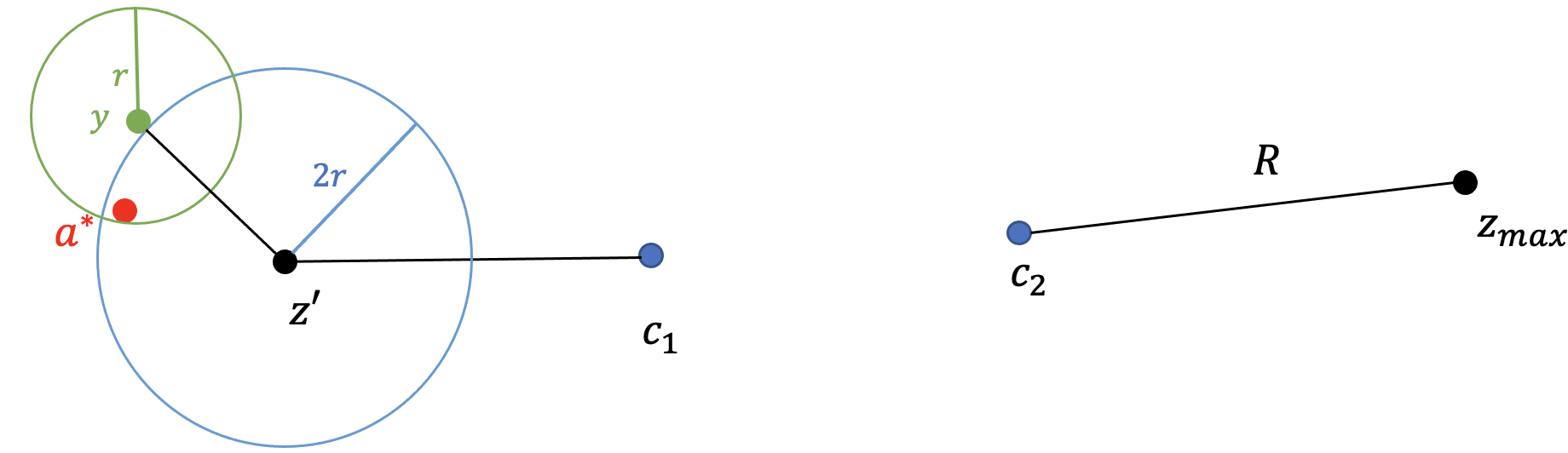
Let $\epsilon>0$ be a constant. Their algorithm runs in $O(1/\epsilon)$ iterations. The $i$ ’th iteration starts from some point $m_{i}$ and uses $O(n)$ time to search for the point $p_{i+1}=\mbox{FN}(P,m_{i})$ furthest from $m_{i}.$ The iteration then selects a “good” point $m_{i+1}$ on the line segment $p_{i+1}m_{i}$ as the starting point for the next iteration, where “good” means that the distance from $m_{i+1}$ to the optimal center is somehow bounded. The time to select such a "good" point is $O(D)$ . The total running time of their algorithm is $O(nD/\epsilon)$ . They also prove that the performance ratio of their algorithm is at most $(1+\epsilon)$ .

The running time of their algorithm is dominated by the $O(n)$ time required to find the point $\mbox{FN}(P,m_{i})$ . As we will see in Theorem 3.2 below, finding the exact furthest point $\mbox{FN}(P,m_{i})$ was not necessary. This could be replaced by $\mbox{AFN}(P,\epsilon/3,m_{i}).$

The first result is that this minor modification of Kim and Schwarzwald [KS20]’s algorithm still produces a $(1+\epsilon)$ approximation.

Theorem 3.2

Let $P\subset\mathbb{R}^{D}$ be a set of points whose minimum enclosing ball has (unknown) radius $r^{*}.$ Suppose $\mbox{AFN}(P,q,\epsilon)$ can be implemented in $T(\epsilon)$ time.

Let $c,r$ be the values returned by Algorithm 2. Then $P\subset B(c,r)$ and $r\leq(1+\epsilon)r^{*}$ . Thus Algorithm 2 constructs a $(1+\epsilon)$ -approximate solution and it runs in $O\left(DT\left(\frac{\epsilon}{3}\right)\frac{1}{\epsilon}\right)$ time.

Plugging Theorem 2.1 into Theorem 3.2 proves Theorem 1.2 for $k=1$ .

Algorithm 2 Modified MEB(

P,\epsilon

)

Input: A set of points $P$ and a constant $\epsilon>0$ .
Output: A $(1+\epsilon)$ -approximate minimum enclosing ball $B(c,r)$ containing all points in $P$ .
The algorithm presented is just a slight modification of that of [KS20]. The differences are that in [KS20], line 4 was originally $p_{i+1}=\mbox{FN}(P,m_{i})$ and the four $(1+\epsilon/3)$ terms on lines 8 and 9, were all originally $(1+\epsilon).$

1:Arbitrarily select a point

p_{1}

from

P

;

2:Set

m_{1}=p_{1}

r=\infty

, and

\delta_{1}=1

;

3:for

i=1

\lfloor 6/\epsilon\rfloor

p_{i+1}=

AFN

(P,m_{i},\epsilon/3)

;

r_{i}=\left(1+\frac{\epsilon}{3}\right)d(m_{i},p_{i+1});

6: if

r_{i}<r

then

c=m_{i};

r=r_{i};

m_{i+1}=m_{i}+(p_{i+1}-m_{i})\cdot\frac{\delta_{i}^{2}+(1+\epsilon/3)^{2}-1}{2(1+\epsilon/3)^{2}}

\delta_{i+1}=\sqrt{1-\left(\frac{1+(1+\epsilon/3)^{2}-\delta^{2}_{i}}{2(1+\epsilon/3)}\right)^{2}}

;

Proof

Every ball $B(m_{i},r_{i})$ generated by Algorithm 2 encloses all of the points in $P,$ i.e.,

\forall i,\quad\max_{p\in P}d(m_{i},p)\leqslant r_{i}.

(3)

To prove the correctness of the algorithm it suffices to show that $r\leq(1+\epsilon)r^{*}.$ Without loss of generality, we assume that $\epsilon\leqslant 1.$

Each iteration of lines 4-9 of $\mbox{MEB}(P,\epsilon)$ must end in one of the two following cases:

(1)

$d(m_{i},p_{i+1})\leqslant(1+\epsilon/3)r^{*}$ ,
(2)

$d(m_{i},p_{i+1})>(1+\epsilon/3)r^{*}$ .

Note that if Case (1) holds for some $i,$ then, directly from Equation 3 (using $\epsilon\leqslant 1$ ),

\max_{p\in P}d(m_{i},p)\leqslant r_{i}=(1+\epsilon/3)d(m_{i},p_{i+1})\leqslant(1+\epsilon/3)^{2}r^{*}<(1+\epsilon)r^{*}

This implies that if Case 1 ever holds, Algorithm 2 is correct.

The main lemma is

Lemma 7

If, $\forall 1\leqslant i\leqslant j$ , case (2) holds, i.e., $d(m_{i},p_{i+1})>(1+\epsilon/3)r^{*}$ , then $j\leq\frac{6}{\epsilon}-1.$

The proof of Lemma 7 is just a straightforward modification of the proof given in Kim and Schwarzwald [KS20] for their original algorithm and is therefore omitted. For completeness we provide the full modified proof in Section 0.D.1.

Lemma 7 implies that, by the end of the algorithm, Case 1 must have occurred at least once, so $r\leq(1+\epsilon)r^{*}$ and the algorithm outputs a correct solution. Derivation of the running time of the algorithm is straightforward, completing the proof of Theorem 3.2.

[KS20] discuss (without providing details) how to use the "guessing" technique of [BHPI02, BC03]) to extend their MEB algorithm to yield a $(1+\epsilon)$ -approximation solution to the $k$ -center problem for $k\geqslant 2$ .

For MEB, the Euclidean $1$ -center, in each iteration, they maintained the location of a candidate center $c$ and computed a furthest point to $c$ among $P$ . For the Euclidean $k$ -centers, in each step, they maintain locations of a set $C$ of candidate centers, $|C|\leqslant k$ and compute a furthest point to $C$ among $P$ using a $\mbox{FN}(P,C)$ procedure.

Again we can modify their algorithm by replacing the $\mbox{FN}(P,C)$ procedure by a $\mbox{AFN}(P,C,\epsilon)$ one, computing an approximate furthest point to $C$ among $P$ . This will prove Theorem 1.2.

The full details of a modified version of their algorithm have been provided in section 0.D.2, which uses $\mbox{AFN}(P,C,\epsilon)$ in place of $\mbox{FN}(P,C)$ , as well as an analysis of correctness and run time.

4 Conclusion

Our main new technical contribution is an algorithm, $\mbox{AFN}(P,C,\epsilon)$ that finds a $(1+\epsilon)$ -approximate furthest point in $P$ to $C.$ This works on top of a navigating net data structure [KL04] storing $P.$

The proofs of Theorems 1.1 and 1.2 follow immediately by maintaining a navigating net and plugging $\mbox{AFN}(P,C,\epsilon)$ into Theorems 3.1 and 0.D.1, respectively.

These provide a fully dynamic and deterministic $(2+\epsilon)$ -approximation algorithm for the $k$ -center problem in a metric space with finite doubling dimension and a $(1+\epsilon)$ -approximation algorithm for the Euclidean $k$ -center problem, where $\epsilon,k$ are parameters given at query time.

One limitation of our algorithm is that, because $\mbox{AFN}(P,C,\epsilon)$ is built on top of navigating nets, it depends upon aspect ratio $\Delta$ . This is the only dependence of the $k$ -center algorithm on $\Delta.$ An interesting future direction would be to develop algorithms for $\mbox{AFN}(P,C,\epsilon)$ in special metric spaces built on top of other structures that are independent of $\Delta.$ This would automatically lead to algorithms for approximate $k$ -center that, in those spaces, would also be independent of $\Delta.$

References

[AS10] Pankaj K Agarwal and R Sharathkumar. Streaming algorithms for extent problems in high dimensions. In Proceedings of the twenty-first annual ACM-SIAM symposium on Discrete algorithms, pages 1481–1489. SIAM, 2010.
[BC03] Mihai Badoiu and Kenneth L Clarkson. Smaller core-sets for balls. In Proceedings of the fifteenth annual ACM-SIAM symposium on Discrete algorithms (SODA), volume 3, pages 801–802, 2003.
[BEJM21] Mohammad Hossein Bateni, Hossein Esfandiari, Rajesh Jayaram, and Vahab Mirrokni. Optimal fully dynamic $k$ -centers clustering. arXiv preprint arXiv:2112.07050, 2021.
[Bes96] Sergei Bespamyatnikh. Dynamic algorithms for approximate neighbor searching. In 8th Canadian Conference on Computational Geometry (CCCG’96), pages 252–257, 1996.
[BHPI02] Mihai Bādoiu, Sariel Har-Peled, and Piotr Indyk. Approximate clustering via core-sets. In Proceedings of the thiry-fourth annual ACM symposium on Theory of computing (STOC), pages 250–257, 2002.
[CGS18] TH Hubert Chan, Arnaud Guerqin, and Mauro Sozio. Fully dynamic k-center clustering. In Proceedings of the 2018 World Wide Web Conference (WWW), pages 579–587, 2018.
[Cha09] Timothy M Chan. Dynamic coresets. Discrete & Computational Geometry, 42(3):469–488, 2009.
[Cha16] Timothy M Chan. Dynamic streaming algorithms for epsilon-kernels. In 32nd International Symposium on Computational Geometry (SoCG 2016). Schloss Dagstuhl-Leibniz-Zentrum fuer Informatik, 2016.
[FG88] Tomás Feder and Daniel Greene. Optimal algorithms for approximate clustering. In Proceedings of the twentieth annual ACM symposium on Theory of computing, pages 434–444, 1988.
[GHL⁺21] Gramoz Goranci, Monika Henzinger, Dariusz Leniowski, Christian Schulz, and Alexander Svozil. Fully dynamic k-center clustering in low dimensional metrics. In 2021 Proceedings of the Workshop on Algorithm Engineering and Experiments (ALENEX), pages 143–153. SIAM, 2021.
[Gon85] Teofilo F Gonzalez. Clustering to minimize the maximum intercluster distance. Theoretical Computer Science, 38:293–306, 1985.
[H⁺01] Juha Heinonen et al. Lectures on analysis on metric spaces. Springer Science & Business Media, 2001.
[HN79] Wen-Lian Hsu and George L Nemhauser. Easy and hard bottleneck location problems. Discrete Applied Mathematics, 1(3):209–215, 1979.
[HS85] Dorit S Hochbaum and David B Shmoys. A best possible heuristic for the k-center problem. Mathematics of operations research, 10(2):180–184, 1985.
[KA15] Sang-Sub Kim and HeeKap Ahn. An improved data stream algorithm for clustering. Computational Geometry, 48(9):635–645, 2015.
[KL04] Robert Krauthgamer and James R Lee. Navigating nets: Simple algorithms for proximity search. In Proceedings of the fifteenth annual ACM-SIAM symposium on Discrete algorithms (SODA), pages 798–807, 2004.
[KS20] Sang-Sub Kim and Barbara Schwarzwald. A (1+ $\varepsilon$ )-approximation for the minimum enclosing ball problem in $R^{d}$ . In the 36th European Workshop on Computational Geometry (EuroCG), 2020.
[PSSS15] Rasmus Pagh, Francesco Silvestri, Johan Sivertsen, and Matthew Skala. Approximate furthest neighbor in high dimensions. In International Conference on Similarity Search and Applications, pages 3–14. Springer, 2015.
[SS19] Melanie Schmidt and Christian Sohler. Fully dynamic hierarchical diameter k-clustering and k-center. arXiv preprint arXiv:1908.02645, 2019.

Appendix 0.A A Navigating Nets Example

Appendix 0.B The Proof of Theorem 2.1

Proof

It only remains to show that the running time of $\mbox{AFN}(P,C,\epsilon)$ is bounded by $O(|C|\log\Delta)+O(|C|(1/\epsilon)^{O(\dim(\mathcal{X}))})$ . We do this by splitting the set of scales $r$ processed by line 2 of Algorithm 1 into two ranges, (1) $\frac{r}{3}\geqslant\max_{x\in P}d(x,C)$ and (2) $\frac{r}{3}<\max_{x\in P}d(x,C).$

We then study the two cases separately : For (1) we will show a better bound on $|Z_{r}|$ than Lemma 5; for (2) we will show that the number of processed scales is small.

(1)

When $\frac{r}{3}\geqslant\max_{x\in P}d(x,C)$ , the size of $Z_{r}$ is small. To see this note that

$\max_{z\in Z_{r}}d(z,C)\leqslant\max_{x\in P}d(x,C)\leqslant\frac{r}{3}$

Thus, for each $z\in Z_{r}$ , there exists a $c\in C$ such that $z\in B(c,\frac{r}{3})$ , i.e., $Z_{r}\subseteq\bigcup_{c\in C}B(c,\frac{r}{3})$ . Additionally, $Z_{r}\subseteq Y_{r}$ , so, $\forall x,y\in Z_{r}$ , $d(x,y)\geqslant r$ . Since the diameter of the ball $B(c,\frac{r}{3})$ is smaller than $r$ , $|Z_{r}\cap B(c,\frac{r}{3})|\leqslant 1$ for every $c\in C$ . Therefore, $|Z_{r}|\leqslant|C|$ .

By Lemma 6, the number of iterations is at most $\log\Delta+O(1)$ . Hence, the total running time for Case (1) is $O(|C|(\log\Delta+1))=O(|C|\log\Delta).$

(2)

When $\frac{r}{3}<\max_{x\in P}d(x,C)$ , although the size of $Z_{r}$ can be larger, the number of possible iterations will be small.

By Lemma 5, $|Z_{r}|\leqslant 4|C|(\gamma+2/\epsilon)^{O(\dim(\mathcal{X}))}$ . Let $r^{\prime}$ be the value when the algorithm terminates, then $2r^{\prime}>\frac{\epsilon}{2}\max_{z\in Z_{r^{\prime}}}d(z,C)$ . From Lemma 4, $(1+\epsilon)\max_{z\in Z_{r^{\prime}}}d(z,C)\geqslant\max_{x\in P}d(x,C)$ .We have

3\cdot\max_{x\in P}d(x,C)>r\geqslant r^{\prime}>\frac{\epsilon}{4}\max_{z\in Z_{r^{\prime}}}d(x,C)\geq\frac{\epsilon}{4(1+\epsilon)}\max_{x\in P}d(x,C)

Thus, the total number of Case (2) iterations is at most $O(\log(\frac{1}{\epsilon}))$ and the total running time in Case (2) is $O(|C|(4(\gamma+2/\epsilon))^{O(\dim(\mathcal{X}))}\log(1/\epsilon)).$

Combining (1) and (2), the total running time of the algorithm is $O(|C|(\log\Delta))+O\left(|C|(1/\epsilon)^{O(\dim(\mathcal{X}))}\right).$

Appendix 0.C The Modified Version of Gonzales’s Greedy Algorithm

As noted in the main text, Algorithm 3 is essentially Gonzalez’s [Gon85] original algorithm with $\mbox{FN}(P,C)$ replaced by $\mbox{AFN}(P,C,\epsilon/5).$

0.C.1 The Algorithm

Algorithm 3 Modified Greedy Algorithm:

GREEDY(P,\epsilon)

Input: A set of points $P\subset X$ , positive integer $k$ and a constant $\epsilon>0$ .
Output: A set $C$ ( $|C|\leq k$ ) and radius $r$ such that $P\subset\bigcup_{c\in C}B(c,r)$ and $r\leq(2+\epsilon)r^{*}.$

1:Arbitrarily select a point

p_{1}

from

P

and set

C=\{p_{1}\}

2:while

|C|<k

C=C\cup\left\{\mbox{AFN}\left(P,C,\frac{\epsilon}{5}\right)\right\}

\mbox{FN}(P,C)

is replaced by

\mbox{AFN}(P,C,\epsilon/5)

4:Set

r=\left(1+\frac{\epsilon}{5}\right)d(C,\mbox{AFN}(P,C,\frac{\epsilon}{5}))

5:Return

C,r

as the solution.

Gonzalaz’s original algorithm only returned $C,$ since in the deterministic case $R=\mbox{FN}(P,C)$ could be calculated in $O(kr)$ time.

0.C.2 Proof of Theorem 3.1

As noted this proof is just a modification of the proof of correctness of Gonzalez’s [Gon85] original algorithm (which used $\mbox{FN}(P,C)$ rather than $\mbox{AFN}(P,C,\epsilon/5)$ ).

Proof

(of Theorem 3.1)

Let $C=\{q_{1},...,q_{k}\}$ and $r$ denote the solution returned by $GREEDY(P,\epsilon)$ .

Let $q=AFN(P,C,\frac{\epsilon}{5})$ be the $(1+\frac{\epsilon}{5})$ -approximate furthest neighbor from $P$ to $C$ returned. Thus

\forall p\in P,\quad d(p,C)\leqslant\left(1+\frac{\epsilon}{5}\right)d(C,q)=r,

i.e., $P\subseteq\bigcup_{i=1}^{k}B(c_{i},r)$ . The output of the algorithm $GREEDY(P,\epsilon)$ is thus a feasible solution.

Let $O=\{o_{1},...,o_{k}\}$ denote an optimal $k$ center solution for the point set $P$ with $r^{*}$ being the optimal radius value. Recall that $|S|$ is the number of points in set $S$ . We consider two cases:

Case 1

$\forall 1\leqslant i\leqslant k$ , $|C\cap B(o_{i},r^{*})|=1$

Fix $p\in P.$ Let $o_{i}$ be such that $p\in B(o_{i},r^{*}).$ Now let $q_{j}$ satisfy $q_{j}\in C\cap B(o_{i},r^{*})$ .

Then, by the triangle inequality, $d(p,q_{j})\leqslant d(p,o_{i})+d(o_{i},q_{j})\leqslant 2r^{*}$ .

We have just shown that $\forall p\in P,$ $d(p,C)\leqslant 2r^{*}$ . In particular,

$d(C,q)\leqslant\max_{p\in P}d(p,C)\leqslant 2r^{*}.$

Therefore,

$r=\left(1+\frac{\epsilon}{5}\right)d(C,q)\leqslant\left(1+\frac{\epsilon}{5}\right)2r^{*}<(2+\epsilon)r^{*}.$

Case 2

There exists $o^{\prime}\in O$ such that $|C\cap B(o^{\prime},r^{*})|\geqslant 2$ .
Let $q_{i}$ be the $i$ th point added into $C$ and $C_{i}=\{q_{1},...,q_{i}\}$ . Thus $C_{1}\subset C_{2}\subset\cdots\subset C_{k}=C$ . In Case 2, $C\cap B(o^{\prime},r^{*})$ contains at least two points $q_{i}$ and $q_{j}$ ( $i<j$ ). From line 3 in $GREEDY(P,\epsilon)$ , we have $q_{j}=AFN\left(P,C_{j-1},\frac{\epsilon}{5}\right)$ . Furthermore,

	$\displaystyle\max_{p\in P}d(p,C)$	$\displaystyle\leqslant\max_{p\in P}d(p,C_{j-1})\quad\quad\%\text{(Because $C_{j-1}\subseteq C$)}$
		$\displaystyle\leqslant\left(1+\frac{\epsilon}{5}\right)d(C_{j-1},q_{j})$
		$\displaystyle\leqslant\left(1+\frac{\epsilon}{5}\right)d(q_{i},q_{j})\quad\quad\%\text{(Because $q_{i}\in C_{j-1}$)}$
		$\displaystyle\leqslant\left(1+\frac{\epsilon}{5}\right)(d(q_{i},o^{\prime})+d(o^{\prime},q_{j}))$
		$\displaystyle\leqslant\left(1+\frac{\epsilon}{5}\right)(r^{}+r^{})=\left(2+\frac{2\epsilon}{5}\right)r^{}.\quad\quad()$

Then, consider the radius returned by $GREEDY(P,\epsilon)$ :

	$\displaystyle r$	$\displaystyle=\left(1+\frac{\epsilon}{5}\right)d(C,q)$
		$\displaystyle\leqslant\left(1+\frac{\epsilon}{5}\right)\max_{p\in P}d(p,C)$
		$\displaystyle\leqslant\left(1+\frac{\epsilon}{5}\right)\left(2+\frac{2\epsilon}{5}\right)r^{}\quad\quad\%\text{(From ($$))}$
		$\displaystyle\leqslant\left(2+\frac{4\epsilon}{5}+\frac{2\epsilon^{2}}{25}\right)\leqslant(2+\epsilon)r^{*}$

where the last inequality assumes, without loss of generality, that $\epsilon\leq 1.$

Thus, $\forall p\in P$ , $P\subseteq\bigcup_{i=1}^{k}B(c_{i},R)$ and, in both cases $r\leqslant(2+\epsilon)r^{*}$ . Thus, $GREEDY(P,\epsilon)$ always computes a $(2+\epsilon)$ -approximation solution.

Appendix 0.D Missing Details Associated with the Modified Kim and Schwarzwald[KS20]’s algorithm

0.D.1 Proof of Lemma 7

As noted previously, this proof is a modification of the proof of correctness given by Kim and Schwarzwald [KS20] for their algorithm (which used $\mbox{FN}(P,q)$ rather than $\mbox{AFN}(P,q,\epsilon/3)$ ).

The proof needs an important geometric observation due to Kim and Schwarzwald[KS20] (slightly rephrased here). This was an extension of an earlier observation by Kim and Ahn[KA15] that was used to design a streaming algorithm for the Euclidean 2-center problem.

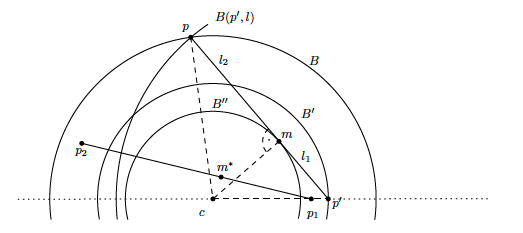
Lemma 8

[KS20] (See Figure 4.) Fix $D\geq 2.$ Let $B$ and $B^{\prime}$ be two $D$ -dimensional balls with radii $r$ and $r^{\prime},$ $r>r^{\prime},$ around the same center point $c$ . Let $p\in\partial B$ and $p^{\prime}\in\partial B^{\prime}$ with $d(p,p^{\prime})=l\geqslant r$ .

Define $B^{\prime\prime}$ to be the $D$ -dimensional ball centered at $c$ that is tangential to $pp^{\prime}$ . Denote that tangent point as $m$ and define the distances $l_{1}=d(p^{\prime},m)$ and $l_{2}=d(p,m)$ . Note that $l=l_{1}+l_{2}$ .

Consider any line segment $p_{1}p_{2}$ satisfying $d(p_{1},p_{2})>l$ , $p_{1}\in B^{\prime}$ and $p_{2}\in B$ . Then any point $m^{*}$ on $p_{1}p_{2}$ with $d(m^{*},p_{1})\geqslant l_{1}$ and $d(m^{*},p_{2})\geqslant l_{2}$ lies inside $B^{\prime\prime}$ .

Lemma 8 will imply that if case (2) $d(m_{i},p_{i+1})>(1+\epsilon/3)r^{*}$ always occurs, then the distance from $c^{*}$ to $m_{i}$ is bounded.

Corollary 1

If, $\forall 1\leqslant i\leqslant j$ , case (2) holds, i.e., $d(m_{i},p_{i+1})>(1+\epsilon/3)r^{*}$ , then $d(c^{*},m_{j+1})\leqslant\delta_{j+1}\cdot r^{*}$ and $\delta_{j+1}<\delta_{j}.$

Proof

The proof will be by induction. In the base case, $\delta_{1}=1$ and $m_{1}$ is arbitrarily selected in $P$ , so $d(c^{*},m_{1})\leqslant\max_{x\in P}d(c^{*},x)=r^{*}=\delta_{1}\cdot r^{*}$ .

Now suppose that, $\forall 1\leqslant i\leqslant j$ , $d(m_{i},p_{i+1})>(1+\epsilon/3)r^{*}$ holds. From the induction hypothesis, we assume that $d(c^{*},m_{j})\leqslant\delta_{j}\cdot r^{*}$ and $\delta_{j+1}<\delta_{j}\leq 1.$

Set $B=B(c^{*},r^{*})$ , and $B^{\prime}=B(c^{*},\delta_{j}r^{*})$ .

Next, arbitrarily select a point $p$ on the boundary of $B(c^{*},r^{*}).$ Now construct ball $\bar{B}=B(p,(1+\epsilon/3)r^{*})$ . From the induction hypothesis,

d(m_{j},p_{j+1})\leqslant d(c^{*},m_{j})+r^{*}\leqslant\delta_{j}r^{*}+r^{*}.

If $\delta_{j}r^{*}\leq(\epsilon/3)r^{*},$ this would imply

d(m_{j},p_{j+1})\leqslant(1+\epsilon/3)r^{*},

contradicting that this is Case 2. Thus $\delta_{j}r^{*}>(\epsilon/3)r^{*}$ .

Since, $\delta_{j}<1,$ this implies that $\bar{B}$ must intersect $B^{\prime}$ . Arbitrarily select one of the two intersection points as $p^{\prime}$ . Next set $l=d(p,p^{\prime})=(1+\epsilon/3)r^{*}.$

Finally, define $B^{\prime\prime}$ to be the ball centered at $c^{*}$ that is tangent to line segment $pp^{\prime}$ . Denote that tangent point as $m$ and define the distances $l_{1}=d(p^{\prime},m)$ and $l_{2}=d(p,m)$ . We will show that $B^{\prime\prime}=B(c^{*},\delta_{j+1}r^{*})$ , i.e., that $d(c^{*},m)=\delta_{j+1}r^{*}$ , where $\delta_{j+1}$ is as defined on line 9 of Algorithm 2.

Note that $l=l_{1}+l_{2}$ . Thus, $l_{1}$ can be computed by the equation (illustrated in figure 5).

(\delta_{j}r^{*})^{2}-l_{1}^{2}=(r^{*})^{2}-((1+\epsilon/3)r^{*}-l_{1})^{2}

This solves to $l_{1}=\frac{\delta_{j}^{2}+(1+\epsilon/3)^{2}-1}{2(1+\epsilon/3)}\cdot r^{*}.$ Thus

\delta_{j+1}=\sqrt{1-\left(\frac{1+(1+\epsilon/3)^{2}-\delta^{2}_{j}}{2(1+\epsilon/3)}\right)^{2}}

as required and, by construction, $\delta_{j+1}<\delta_{j}.$ Furthermore,

\frac{\delta_{i}^{2}+(1+\epsilon/3)^{2}-1}{2(1+\epsilon/3)^{2}}=\frac{l_{1}}{l}.

Plugging into line 8 of Algorithm 2 yields

m_{j+1}=m_{j}+(p_{j+1}-m_{j})\cdot\frac{l_{1}}{l}=m_{j}+(p_{j+1}-m_{j})\cdot\left(1-\frac{l_{2}}{l}\right).

Since $d(m_{j},p_{j+1})>(1+\epsilon/3)r^{*}$ , we have

d(m_{j},m_{j+1})=\frac{l_{1}}{l}\cdot d(m_{j},p_{j+1})>\frac{l_{1}}{(1+\epsilon/3)r^{*}}(1+\epsilon/3)r^{*}=l_{1}

and $d(p_{j+1},m_{j+1})=\frac{l_{2}}{l}\cdot d(m_{j},p_{j+1})>l_{2}$ .

From the induction hypothesis, $d(c^{*},m_{j})\leqslant\delta_{j}\cdot r^{*}$ , so $m_{j}\in B(c^{*},\delta_{j}r^{*})$ . The definition of $c^{*},r^{*},$ further implies $p_{j+1}\in B(c^{*},r^{*})$ .

We now apply Lemma 8, with $p_{1}=m_{j}$ , $p_{2}=p_{j+1}$ and $m^{*}=m_{j+1}.$ Since these three points are collinear, Lemma 8 implies that $m^{*}\in B^{\prime\prime},$ i.e., that

d(c^{*},m_{j+1})\leqslant\delta_{j+1}\cdot r^{*}.

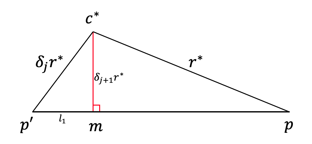
We can now prove Lemma 7. We again note that this is just a slight modification of the proof given by Kim and Schwarzwald [KS20] for their original algorithm.

Proof

(of Lemma 7.)

Recall that the goal is to prove that if, $\forall 1\leqslant i\leqslant j$ , case (2) holds, i.e., $d(m_{i},p_{i+1})>(1+\epsilon/3)r^{*}$ , then $j\leq\frac{6}{\epsilon}-1.$

Consider the triangle $\bigtriangleup pp^{\prime}c^{*}$ (Figure 5) constructed in the proof of Corollary 1.

Let $p(i),p^{\prime}(i),m(i)$ denote $p,p^{\prime},m$ in step $i$ of the algorithm.

Recall that in the construction, $p(i)$ is on the boundary of $B(c^{*},r^{*})$ and $p^{\prime}(i)$ is on the boundary of $B^{\prime}=B(c^{*},\delta_{i}r^{*})$ . Additionally, $d(p(i),p^{\prime}(i))=(1+\epsilon/3)r^{*}$ and line segment $c^{*}m$ is vertical to line segment $p(i)p^{\prime}(i).$ Recall that

d(p^{\prime}(i),m(i))=l_{1}=\frac{\delta_{i}^{2}+(1+\epsilon/3)^{2}-1}{2(1+\epsilon/3)}r^{*}\quad\mbox{and}\quad d(p(i),m(i))=(1-\epsilon/3)r^{*}-l_{1}.

Now define $\beta_{i},\alpha_{i}$ so that

d(m(i),p(i))=\beta_{i}\cdot d(p(i),p^{\prime}(i))=\beta_{i}(1+\epsilon/3)r^{*}\quad\mbox{and}\quad(p^{\prime}(i),m(i))=\alpha_{i}(1+\epsilon/3)r^{*}.

Note that $\alpha_{i}+\beta_{i}=1.$

Since $\bigtriangleup m(i)p(i)c^{*}$ is a right triangle, $d(m(i),p(i))=\beta_{i}(1+\epsilon/3)r^{*}\leqslant d(c^{*},p(i))=r^{*}$ so, $\forall i,$ $\beta_{i}\leq\frac{1}{(1+\epsilon/3)}$ .

We have therefore just proven that if, $\forall 1\leqslant i\leqslant j$ , case (2) holds, i.e., $d(m_{i},p_{i+1})>(1+\epsilon/3)r^{*}$ , then for all such $i,$ $\beta_{i}\leq\frac{1}{(1+\epsilon/3)}$ and, in particular, $\beta_{j}\leq\frac{1}{(1+\epsilon/3)}.$

By construction, $(\delta_{i}r^{*})^{2}=(r^{*})^{2}-(\beta_{i}(1+\epsilon/3)r^{*})^{2}$ and $(\alpha_{i}(1+\epsilon/3)r^{*})^{2}=(\delta_{i-1}r^{*})^{2}-(\delta_{i}r^{*})^{2}$ . Plugging the first (twice) into the second yields

(\alpha_{i}(1+\epsilon/3)r^{*})^{2}=\left((r^{*})^{2}-(\beta_{i-1}(1+\epsilon/3)r^{*})^{2}\right)-\left((r^{*})^{2}-(\beta_{i}(1+\epsilon/3)r^{*})^{2}\right),

or $\beta_{i}^{2}=\alpha_{i}^{2}+\beta_{i-1}^{2}.$

Combining this with $\beta_{i}=1-\alpha_{i}$ yields $\beta_{i}=\frac{1+\beta^{2}_{i-1}}{2}$ . Set $\varphi_{i}=\frac{1}{1-\beta_{i}}$ . Then

\varphi_{i}=\frac{1}{1-\beta_{i}}=\frac{1}{1-\frac{1+\beta_{i-1}^{2}}{2}}=\frac{1}{\frac{1-\beta_{i-1}^{2}}{2}}=\frac{\frac{1}{1-\beta_{i-1}}}{\frac{1+\beta_{i-1}}{2}}=\frac{\varphi_{i-1}}{\frac{1+(1-\frac{1}{\varphi_{i-1}})}{2}}=\frac{\varphi_{i-1}}{1-\frac{1}{2\varphi_{i-1}}}.

Thus

\varphi_{i}=\frac{\varphi_{i-1}}{1-\frac{1}{2\varphi_{i-1}}}=\varphi_{i-1}(1+\frac{1}{2\varphi_{i-1}}+\frac{1}{(2\varphi_{i-1})^{2}}+\cdots)\geqslant\varphi_{i-1}+\frac{1}{2}.

Recall that $\delta_{1}=1$ , $d(c^{*},p(1))=d(c^{*},p^{\prime}(1))=r^{*}$ , i.e., $\bigtriangleup m(i)p(i)c^{*}$ is an isosceles triangle. Therefore, $\alpha_{1}=\beta_{1}=\frac{1}{2},$ and $\varphi_{1}=2.$ Iterating the equation above yields $\varphi_{i}\geqslant 2+\frac{i-1}{2}$ . Thus, $\beta_{i}\geqslant 1-\frac{2}{3+i}$ . Thus, if $j>\frac{6}{\epsilon}-1$ , then $\beta_{j}>\frac{1}{1+\epsilon/3},$ which we previously saw was not possible.

0.D.2 The Actual Modified Algorithm for Euclidean $k$ Center

Algorithm 4 Modified

k

-center(

P,\epsilon,k

)

Input: A set of points $P$ , positive integer $k$ and a constant $\epsilon>0$ .
Output: A set $\bar{C}$ ( $|\bar{C}|\leq k$ ) and radius $\bar{r}$ such that $P\subset\bigcup_{c\in\bar{C}}B(c,r)$ and $\bar{r}\leq(1+\epsilon)r^{*}.$
In the algorithm, each $m_{j,i}$ , $j\in\{1,\ldots,k\},$ is either undefined or a point in $\mathbb{R}^{D}.$ $M_{i}$ denotes the set of defined $m_{j,i}.$ $\mathcal{F}$ is the set of all functions from $\{1,\ldots,k\lfloor 6/\epsilon\rfloor\}$ to $\{1,\ldots,k\}.$

\bar{r}=\infty

2:for every function

f\in\mathcal{F}

\forall j\in\{1\ldots k\},

set

\delta_{j,1}=1;

Set

r=\infty;

4: Arbitrarily select a point

p_{1}

from

P

;

m_{j,1}=\begin{cases}\mbox{undefined}&\mbox{if $j\not=f(1)$}\\ p_{1}&\mbox{if $j=f(1)$}\end{cases}

6: for

i=1

k\lfloor 6/\epsilon\rfloor

p_{i+1}=

AFN

(P,M_{i},\epsilon/3)

;

r_{i}=\left(1+\frac{\epsilon}{3}\right)d(M_{i},p_{i+1});

9: if

r_{i}<r

then

10:

C=M_{i}

;

r=r_{i}

;

11:

m_{j,i+1}=\begin{cases}m_{j,i}&\mbox{if $j\not=f(i)$}\\ m_{j,i}+(p_{i+1}-m_{j,i})\cdot\frac{\delta_{j,i}^{2}+(1+\epsilon/3)^{2}-1}{2(1+\epsilon/3)^{2}}&\mbox{if $j=f(i)$}\end{cases}

12:

\delta_{j,i+1}=\begin{cases}\delta_{j,i}&\mbox{if $j\not=f(i)$}\\ \sqrt{1-\left(\frac{1+(1+\epsilon/3)^{2}-\delta^{2}_{j,i}}{2(1+\epsilon/3)}\right)^{2}}&\mbox{if $j=f(i)$}\end{cases}

13: if

r<\bar{r}

then

14:

\bar{r}=r;

\bar{C}=C;

Before starting, we provide a brief intuition. If, for each $p\in P$ , the algorithm knew in advance in which of the $k$ clusters $p$ is located, it could solve the problem by running Algorithm 2 separately for each cluster and returning the largest radius it found. Since it doesn’t know that information in advance, it “guesses” the location. This guess is encoded by the function $f\in{\mathcal{F}}$ introduced in Algorithm 4. It runs this procedure for every possible guess. Since one of the guesses must be correct, the algorithm returns a correct answer.

Again, we emphasize that Algorithm 4 is essentially the algorithm alluded²²2We write “alluded to” because [KS20] do not actually provide details. They only say that they are utilizing the guessing technique from [BC03]. In our algorithm, we have provided full details of how this can be done. to in Kim and Schwarzwald [KS20] with calls to $\mbox{FN}(P,C)$ replaced by calls to $\mbox{AFN}(P,C,\epsilon/3).$

Theorem 0.D.1

Let $P\subset\mathbb{R}^{D}$ be a finite set of points. Suppose $\mbox{AFN}(P,C,\epsilon)$ can be implemented in $T(|C|,\epsilon)$ time. Then an $(1+\epsilon)$ -approximate $k$ -center solution for $P$ can be constructed in $O\left(DT\left(k,\frac{\epsilon}{3}\right)2^{O(k\log k/\epsilon)}\right)$ time.

Proof

Let $C^{*}=\{c_{1}^{*},\ldots,c^{*}_{k}\}$ be a set of optimal centers and $r^{*}=d(C^{*},P).$ Partition the points in $P$ into $P_{i},$ $i=1,\ldots,k,$ so that $P_{i}\subseteq P\cap B(c^{*}_{i},r^{*}).$ Let $r^{*}_{i}=d(c^{*}_{i},P_{i}),$ i.e., $B(c^{*}_{i},r^{*}_{i})$ is a minimum enclosing ball for $P_{i}.$ Note that $r^{*}=\max_{i}r^{*}_{i}.$

Fix $f:\{1,\ldots,k\lfloor 6/\epsilon\rfloor\}\rightarrow\{1,\ldots,k\}$ to be some arbitrary function. Lines 3-12 of Algorithm 4 maintains a list of $k$ tentative centers; $m_{1,i},\ldots,m_{k,i},$ denotes the list at the start of iteration $i.$ Note that some of the $m_{j,i}$ might be undefined, i.e., do not exist. $M_{i}$ will denote the set of defined items in the list at the start of iteration $i.$ During iteration $i$ , the list updates (only the) tentative center $m_{f(i),i}$ and also constructs a radius $r_{i}.$

The algorithm starts with all of the $m_{j,i}$ being undefined, chooses some arbitrary point of $P,$ calls it $p_{1},$ and then sets $m_{f(1),1}=p_{1}.$

At step $i,$ it sets $p_{i+1}=\mbox{AFN}\left(P,M_{i},\epsilon/3\right)$ and $r_{i}=\left(1+\frac{\epsilon}{3}\right)d(M_{i},p_{i+1}).$

Note that the definitions of $\mbox{AFN}\left(P,M_{i},\epsilon/3\right)$ and $r_{i}$ immediately imply

\forall i,\quad P\subset\bigcup_{q\in M_{i}}B(q,r_{i}).

(4)

Thus, lines 3-12 return $C$ and $r$ that cover all points in $P$ in $O\left(D\frac{k}{\epsilon}T\left(|C|,\frac{\epsilon}{3}\right)\right)$ time.

So far, the analysis has not considered lines 11-12 of the algorithm.

The algorithm arbitrarily chooses $p_{1}.$ Now consider the unique function $f^{\prime}(i)$ that always returns the index of the $P_{j}$ that contains $p_{i+1},$ i.e., $p_{i+1}\in P_{f^{\prime}(i)}.$ For this $f^{\prime}(i),$ lines 11 and 12 of the algorithm work as if they are running the original modified MEB algorithm on each of the $P_{j}$ separately.

By the generalized pigeonhole principle, there must exist at least one index $j$ such that $f^{\prime}(i)=j$ at least $\lfloor 6/\epsilon\rfloor$ times. For such a $j,$ consider the value of $i$ for which $f^{\prime}(i)=j$ exactly $\lfloor 6/\epsilon\rfloor$ times. Then, from the analysis of Algorithm 2, for this particular $j,$

d(m_{j,i},p_{i+1})\leq(1+\epsilon/3)r^{*}_{j},

d(M_{i},p_{i+1})\leq d(m_{j,i},p_{i+1})\leq(1+\epsilon/3)r^{*}_{j}\leq(1+\epsilon/3)r^{*}.

Thus

r_{i}=\left(1+\frac{\epsilon}{3}\right)d(M,p_{i+1})\leq\left(1+\frac{\epsilon}{3}\right)^{2}r^{*}\leq\left(1+\epsilon\right)r^{*}.

In particular, lines 3-12 using $f^{\prime}(i)$ returns a $(1+\epsilon)$ -approximate solution.

Algorithm 4 runs lines 3-12 on all $\Theta\left(k^{k\lfloor 6/\epsilon\rfloor}\right)=2^{O(k\log k/\epsilon)}$ different possible functions $f(i).$ Since this includes $f^{\prime}(i),$ the full algorithm also returns a $(1+\epsilon)$ -approximate solution.

Fully Dynamic kk-Center in Low Dimensions via Approximate Furthest Neighbors

Abstract

Keywords:

1 Introduction

Static algorithms

Dynamic algorithms

Our contributions and techniques

Theorem 1.1

Theorem 1.2

2 Searching for a (1+ϵ)(1+\epsilon)-Approximate Furthest Point in a Dynamically Changing Point Set

Definition 1

Definition 2 (Doubling Dimensions)

Theorem 2.1

2.1 Navigating Nets [KL04]

Lemma 1

Definition 3 (rr-net)

Lemma 2

Theorem 2.2

2.2 The Approximate Furthest Neighbor Algorithm AFN(P,C,ϵ\mbox{AFN}(P,C,\epsilon)

Definition 4 (The sets ZrZ_{r})

Lemma 3

Proof

Lemma 4

Proof

Lemma 5

Proof

Lemma 6

Proof

3 Modified kk-Center Algorithms

3.1 A Modified Version of Gonzalez’s [Gon85]’s Greedy Algorithm

Theorem 3.1

3.2 A Modified Version of the Kim Schwarzwald [KS20] Algorithm

Theorem 3.2

Proof

Lemma 7

4 Conclusion

References

Appendix 0.A A Navigating Nets Example

Appendix 0.B The Proof of Theorem 2.1

Proof

Appendix 0.C The Modified Version of Gonzales’s Greedy Algorithm

0.C.1 The Algorithm

0.C.2 Proof of Theorem 3.1

Proof

Appendix 0.D Missing Details Associated with the Modified Kim and Schwarzwald[KS20]’s algorithm

0.D.1 Proof of Lemma 7

Lemma 8

Corollary 1

Proof

Proof

0.D.2 The Actual Modified Algorithm for Euclidean kk Center

Theorem 0.D.1

Proof

Fully Dynamic $k$ -Center in Low Dimensions via Approximate Furthest Neighbors

2 Searching for a $(1+\epsilon)$ -Approximate Furthest Point in a Dynamically Changing Point Set

Definition 3 ( $r$ -net)

2.2 The Approximate Furthest Neighbor Algorithm $\mbox{AFN}(P,C,\epsilon$ )

Definition 4 (The sets $Z_{r}$ )

3 Modified $k$ -Center Algorithms

0.D.2 The Actual Modified Algorithm for Euclidean $k$ Center