Functional Control of Oscillator Networks
Abstract
Oscillatory activity is ubiquitous in natural and engineered network systems. The interaction scheme underlying interdependent oscillatory components governs the emergence of network-wide patterns of synchrony that regulate and enable complex functions. Yet, understanding, and ultimately harnessing, the structure-function relationship in oscillator networks remains an outstanding challenge of modern science. Here, we address this challenge by presenting a principled method to prescribe exact and robust functional configurations from local network interactions through optimal tuning of the oscillators’ parameters. To quantify the behavioral synchrony between coupled oscillators, we introduce the notion of functional pattern, which encodes the pairwise relationships between the oscillators’ phases. Our procedure is computationally efficient and provably correct, accounts for constrained interaction types, and allows to concurrently assign multiple desired functional patterns. Further, we derive algebraic and graph-theoretic conditions to guarantee the feasibility and stability of target functional patterns. These conditions provide an interpretable mapping between the structural constraints and their functional implications in oscillator networks. As a proof of concept, we apply the proposed method to replicate empirically recorded functional relationships from cortical oscillations in a human brain, and to redistribute the active power flow in different models of electrical grids.
Introduction
Complex coordinated behavior of oscillatory components is linked to the function of many natural and technological network systems [17, 58, 15]. For instance, distinctive network-wide patterns of synchrony [72, 31, 71] determine the coordinated motion of orbiting particle systems [87], promote successful mating in populations of fireflies [12], regulate the active power flow in electrical grids [23], predict global climate change phenomena [79], dictate the structural development of mother-of-pearl in mollusks [9], and enable numerous cognitive functions in the brain [14, 26]. Since this rich repertoire of patterns emerges from the properties of the underlying interaction network [73], controlling the collective configuration of interdependent units holds a tremendous potential across science and engineering [75]. Despite its practical significance, a comprehensive method to enforce network-wide patterns of synchrony by intervening on the network’s structural parameters does not yet exist.
In this work, we develop a rigorous framework that allows us to optimally control the spatial organization of the network components and their oscillation frequencies to achieve desired patterns of synchrony. We abstract the rhythmic activity of a system as the output of a network of diffusively coupled oscillators [4, 22] with Kuramoto dynamics. This modeling choice is motivated by the rich dynamical repertoire and wide adoption of Kuramoto oscillators [2]. Specifically, we consider an undirected network of oscillators with dynamics
| (1) |
where and are the frequency and phase of the -th oscillator, respectively, is the weighted adjacency matrix of , and and denote the oscillator and interconnection sets, respectively. In this work we consider the case where the network admits both cooperative (i.e., ) and competitive (i.e., ) [34] interactions among the oscillators, as well as the more constrained case of purely cooperative interactions that arises in several real-word systems. For instance, negative interactions are not physically meaningful in networks of excitatory neurons, in power distribution networks (where the interconnection weight denotes conductance and susceptance of a transmission line), and in urban transportation networks (where interconnections denote the number of vehicles on a road with respect to its maximum capacity).
To quantify the pairwise functional relations between oscillatory units, and inspired by the work in Ref. [5], we define a local correlation metric that, compared to the classical Pearson correlation coefficient, does not depend on sampling time and is more convenient when dealing with periodic phase signals (see Supplementary Information). Given a pair of phase oscillators and with phase trajectories and , we define the correlation coefficient
| (2) |
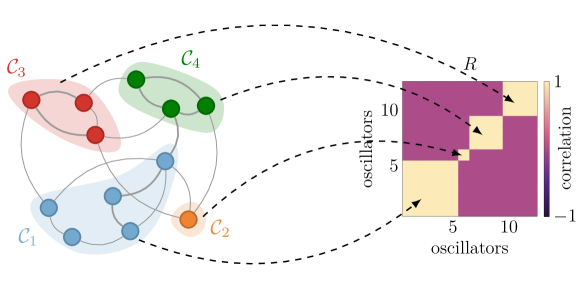
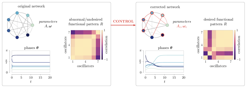
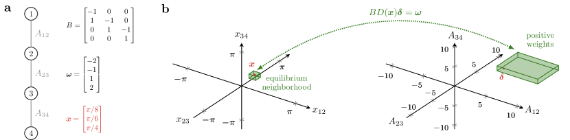
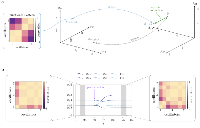
where denotes the average over time. A functional pattern is formally defined as the symmetric matrix whose -th entry equals . Importantly, a functional pattern explicitly encodes the pairwise, local, correlations across all of the oscillators, which are more informative than a global observable (e.g., the order parameter [4, 6]). It is easy to see that, if two oscillators and synchronize after a certain initial transient, as time increases. If two oscillators and become phase-locked (i.e., their phase difference remains constant over time), then their correlation coefficient converges to some constant value with magnitude smaller than 1. If the phases of two oscillators and evolve independently, then their correlation value remains small over time. A few questions arise naturally, which will be answered in this paper. Are all functional patterns achievable? Which network configurations allow for the emergence of multiple target functional patterns? And, if a certain functional pattern can be achieved, is it robust to perturbations? Surprisingly, we reveal that controlling functional patterns can be cast as a convex optimization problem, whose solution can be characterized explicitly. Fig. 1 shows our framework and an example of control of functional pattern for a network with oscillators. In the paper, we will validate our methods by replicating functional patterns from brain recordings in an empirically reconstructed neuronal network, and by controlling the active power distribution in multiple models of power grid.
While synchronization phenomena in oscillator networks have been studied extensively (e.g., see [57, 74, 70, 52, 10]), the development of control methods to impose desired synchronous behaviors has only recently attracted the attention of the research community [55, 25, 28, 45]. Perhaps the work that is closest to our approach is Ref. [25], where the authors tailor interconnection weights and natural frequencies to achieve a specified level of phase cohesiveness in a network of Kuramoto oscillators. Our work improves considerably upon this latter study, whose goal is limited to prescribing an upper bound to the phase differences, by enabling the prescription of pairwise phase differences and by investigating the stability properties of different functional patterns. Taken together, existing results highlight the importance of controlling distinct configurations of synchrony, but remain mainly focused on the control of “macroscopic” observables of synchrony (e.g., the average synchronization level of all the oscillators). In contrast, our control method prescribes desired pairwise levels of correlation across all of the oscillators, thus enabling a precise “microscopic” description of functional interactions.
Analytical results
Feasible functional patterns in positive networks
A functional pattern is an matrix whose entries are the time-averaged cosine of the differences of the oscillator phases (see equation (2)). When the oscillators reach an equilibrium, the differences of the oscillator phases become constant, and the network evolves in a phase-locked configuration. In this case, the functional pattern of the network also becomes constant, and is uniquely characterized by the phase differences at the equilibrium configuration. In this work we study functional patterns for the special case of phase-locked oscillators and, given the equivalence between a desired functional pattern and a desired set of phase differences at equilibrium, convert the problem of generating a functional pattern into the problem of ensuring a desired phase-locked configuration. We recall that, while convenient for the analysis, phase-locked configurations play a crucial role in the functioning of many natural and man-made networks [38, 81, 39].
For the undirected network , let be the difference of the phases of the oscillators and , and let be the vector of all phase differences with and . The network dynamics (1) can be conveniently rewritten in vector form as (see Methods)
| (3) |
where is the (oriented) incidence matrix of the network , is a diagonal matrix of the sine functions in equation (1), and is a vector collecting all the weights with . Because we focus on phase-locked trajectories, all oscillators evolve with the same frequency and the vector satisfies , where is the average of the natural frequencies of the oscillators. Further, since contains only oscillators, any phase difference can always be written as a function of independent differences; for instance, . In fact, for any pair of oscillators and with , it holds . This implies that the vector of all phase differences in equation (3), and in fact any functional pattern, has only degrees of freedom and can be uniquely specified with a set of independent differences (see Methods). Following this reasoning and to avoid cluttered notation, let , and notice that the problem of enforcing a desired functional pattern simplifies to (i) converting the desired functional pattern to the corresponding phase differences , and (ii) computing the network weights to satisfy the following equation:
| (4) |
where we note that the vector has zero mean and that, with a slight abuse of notation, denotes the -dimensional diagonal matrix of the sine of the phase differences uniquely defined by the ()-dimensional vector .
We begin by studying the problem of attaining a desired functional pattern using only nonnegative weights. With the above notation, for a desired functional pattern corresponding to the phase differences , this problem reads as
| (5) | ||||
| (5a) | ||||
| and | (5b) |
It should be noticed that the feasibility of the optimization problem (5) depends on the sign of the entries of the diagonal matrix , but is independent of their magnitude. To see this, notice that
where the and absolute value operators are applied element-wise. Then, Problem (5) is feasible if and only if there exists a nonnegative solution to
The feasibility of the latter equation, in turn, depends on the projections of the natural frequencies on the columns of : a nonnegative solution exists if belongs to the cone generated by the columns of . This also implies that, if a network admits a desired functional pattern then, by tuning its weights, the same network can generate any other functional pattern such that . Thus, by properly tuning its weights, a network can generally generate a continuum of functional patterns determined uniquely by signs of its incidence matrix and the oscillators natural frequencies. This property is illustrated in Fig. 2 for the case of a line network.
A sufficient condition for the feasibility of Problem (5) is as follows:
There exists such that if there exists a set satisfying:
-
(i.a)
for all with and ;
-
(i.b)
for all ;
-
(i.c)
.
Equivalently, the above conditions ensure that is contained within the cone generated by the columns of (see Fig. 3a for a self-contained example). To see this, rewrite the pattern assignment problem as
| (6) |
where the subscripts and denote the entries corresponding to the set and the remaining ones, respectively. If the vectors , , are linearly independent, condition (i.a) implies that is an M-matrix; that is, a matrix which has nonpositive off-diagonal elements and positive principal minors [36]. Otherwise, the argument holds verbatim by replacing with any subset such that the vectors , , are linearly independent. Condition (i.c) guarantees the existence of a solution to . A particular solution to the latter equation is
where denotes the Moore-Penrose pseudo-inverse of a matrix. The positivity of follows from condition (i.b) and the fact that the inverse of an M-matrix is element-wise nonnegative [36]. We conclude that a solution to equation (6) is given by and .
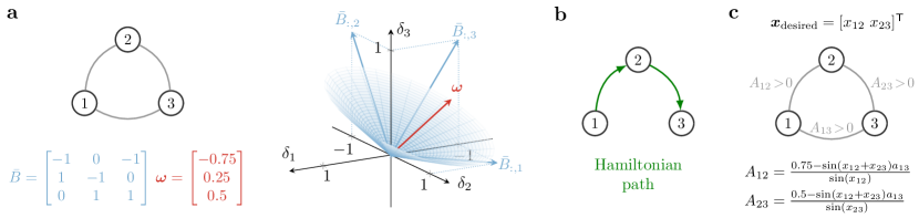
To avoid disconnecting edges or to maintain a fixed network topology, a functional pattern should be realized in Problem (5) using a strictly positive weight vector (that is, rather than ). While, in general, this is a considerably harder problem, a sufficient condition for the existence of a strictly positive solution is that the network with incidence matrix contains an Hamiltonian path, that is, a directed path that visits all the oscillators exactly once (Fig. 3b shows a network containing an Hamiltonian path). Namely,
There exists a strictly positive solution to if
-
(ii.a)
the network with incidence matrix contains a directed Hamiltonian path ;
-
(ii.b)
for all ;
The incidence matrix of a directed Hamiltonian path has two key properties. First, it comprises linearly independent columns, since the path covers all the vertices and contains no cycles. This guarantees that . Second, the columns of the incidence matrix satisfy and for all , . Then, letting the set in the result above identify the columns of the Hamiltonian path, conditions (ii.a) and (ii.b) imply (i.a)-(i.c), thus ensuring the existence of a nonnegative set of weights that solves the pattern assignment problem . Furthermore, by rewriting the pattern assignment problem as in equation (6), the following vector of interconnection weights solves such equation (see Methods):
Because defines an Hamiltonian path and because of (ii.b), the vector contains only strictly positive entries. Thus, for any sufficiently small and positive vector , the weights are also strictly positive, ultimately proving the existence of a strictly positive solution to the pattern assignment problem (see Methods). Fig. 3c illustrates a self-contained example.
Taken together, the results presented in this section reveal that the interplay between the network structure and the oscillators’ natural frequencies dictates whether a desired functional pattern is achievable under the constraint of nonnegative (or even strictly positive) interconnections. First, dense positive networks with a large number of edges are more likely to generate a desired functional pattern, since their incidence matrix features a larger number of candidate vectors to satisfy conditions (i.a)-(i.c). Second, densely connected networks are also more likely to contain an Hamiltonian path, thus promoting also strictly positive network designs. Third, after an appropriate relabeling of the oscillators such that any interconnection from to in the Hamiltonian path satisfies , condition (ii.b) is equivalent to requiring that . That is, the feasibility of a functional pattern is guaranteed when the natural frequencies increase monotonically with the ordering identified by the Hamiltonian path. This also implies, for instance, that sparsely connected positive networks, and not only dense ones, can attain a large variety of functional patterns. An example is a connected line network with increasing natural frequencies, which can generate, among others, any functional pattern defined by phase differences that are smaller than (trivially, when the phase differences are smaller than and the natural frequencies are increasing, a line network contains an Hamiltonian path and the vector of natural frequencies has positive projections onto the columns of the incidence matrix). Fig. 2a contains an example of such a network.
Compatibility of multiple functional patterns
A single choice of the interconnections weights can allow for multiple desired functional patterns, as long as they are compatible with the network dynamics in equation (1). In this section, we provide a characterization of compatible functional patterns in a given network, and derive conditions for the existence of a set of interconnection weights that achieve multiple desired functional patterns. Being able to concurrently assign multiple functional patterns is crucial, for instance, to the investigation and design of memory systems [68], where different patterns of activity correspond to distinct memories. Furthermore, our results complement previous work on the search of equilibria in oscillator networks [44].
To find a set of functional patterns that exists concurrently in a given network with fixed interconnection weights , we exploit the algebraic core of equation (4) and show that the kernel of the incidence matrix uniquely determines the equilibria of the network. In fact, for a given network (i.e., with nonzero components) all compatible equilibria , , must satisfy
| (7) |
From equation (7), we can see that the sine vector of all compatible equilibria must belong to a specific affine subspace of :
| (8) |
Rewriting equation (4) in the above form connects the existence of distinct functional patterns with , the latter featuring a number of well known properties. For instance, it holds that , where is the number of connected components in a network, and that coincides with the subspace spanned by the signed path vectors of all undirected cycles in the network [30]. Notice also that, after a suitable reordering of the phase differences in , we can write , where denotes the phase differences dependent on desired phase differences . Thus, all the for which intersects the affine space described by identify compatible functional patterns.
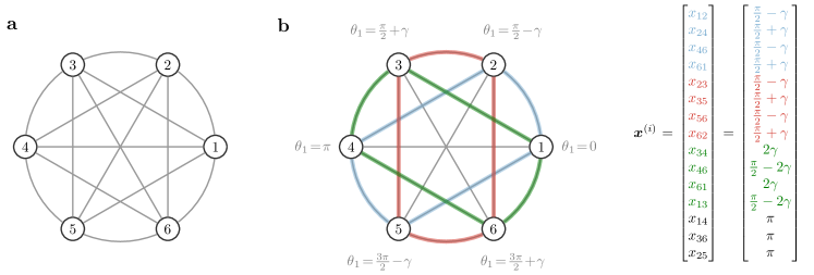
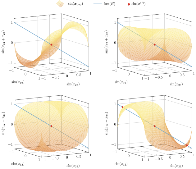
To showcase how the intimate relationship between the network structure and the kernel of its incidence matrix enables the characterization of which (and how many) compatible patterns coexist, we consider three essential network topologies: trees, cycles, and complete graphs. For the sake of simplicity, we let and , so that equation (8) holds whenever . In networks with tree topologies it holds , and is satisfied by patterns of the form , for all . Consider now cycle networks, where . For any cycle of oscillators, two families of patterns are straightforward to derive. First, there are patterns of the form , with , and . Second, there are splay states [22], where the oscillators’ phases evenly span the unitary circle, with , , . Fig. 4 illustrates the compatible functional patterns satisfying equation (8) in a positive network of three fully synchronizing oscillators.
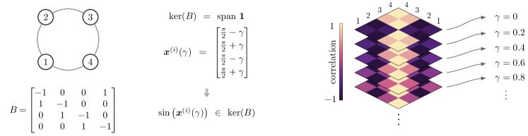
In general, however, cycle networks of identical oscillators admit infinite coexisting patterns. For instance, Fig. 5 shows how we can parameterize infinite equilibria with a scalar in a cycle of oscillators. Finally, as complete graphs are equivalent to a composition of cycles, they also admit infinite compatible patterns that can be parameterized akin to what occurs in a simple cycle (see Supplementary Figure 11).
We now turn our attention to finding the interconnection weights that simultaneously enable a collection of desired functional patterns . We first notice that equation (7) reveals that to achieve a desired functional pattern with components not equal to , , the network weights must belong to an -dimensional affine subspace of :
| (9) |
Let . Then, to concurrently realize a collection of patterns , a solution to equations (9) exists if and only if . It is worth noting that, whenever the latter intersection coincides with a singleton, then there exists a single choice of network weights that realizes . However, if corresponds to a subspace, then infinite networks can realize the desired collection of functional patterns. We conclude by emphasizing that a positive that achieves the desired patterns exists if and only if . That is, if the network weights belong to the nonempty intersection of the affine subspaces with the positive orthant.
Stability of functional patterns
A functional pattern is stable when small deviations of the oscillators phases from the desired configuration lead to vanishing functional perturbations. Stability is a desired property since it guarantees that the desired functional pattern is robust against perturbations to the oscillators dynamics. To study the stability of a functional pattern, we analyze the Jacobian of the Kuramoto dynamics at the desired functional configuration, which reads as [22]
| (10) |
where denotes the Laplacian matrix of the network with weights scaled by the cosines of the phase differences (the weight between nodes and is ). The functional pattern is stable when the eigenvalues of the above Jacobian matrix have negative real parts. For instance, if all phase differences are strictly smaller than (that is, the infinity-norm of satisfies ), then the Jacobian in equation (10) is known to be stable [22]. In the case that both cooperative and competitive interactions are allowed, we can ensure stability of a desired pattern by specifying the network weights in such that if and otherwise, so that the matrix becomes the Laplacian of a positive network (see Methods). Furthermore, we observe that in the particular case where some differences , the network may become disconnected since . Because the Laplacian of a disconnected network has multiple eigenvalues at zero, marginal stability may occur, and phase trajectories may not converge to the desired pattern.
When some phase differences are larger than and the network allows only for nonnegative weights, then stability of a functional pattern is more difficult to assess because the Jacobian matrix becomes a signed Laplacian [86]. The off-diagonal entries of a signed Laplacian satisfy whenever , thus possibly changing the sign of its diagonal entries and violating the conditions for the use of classic results from algebraic graph theory for the stability of Laplacian matrices. To derive a condition for the instability of the Jacobian in equation (10), we exploit the notion of structural balance. We say that the cosine-scaled network with Laplacian matrix is structurally balanced if and only if its oscillators can be partitioned into two sets, and , such that all with connect oscillators in to oscillators in , and all with connect oscillators within , . If a network is structurally balanced, then its Laplacian has mixed eigenvalues [86]. Therefore, we conclude the following:
If the functional pattern yields a structurally balanced cosine-scaled network, then is unstable.
The above condition allows us to immediately assess the instability of functional patterns for the special cases of line and cycle networks. In fact, for a line network with positive weights, is unstable whenever for any . Instead, for a cycle network with positive weights, the pattern can be stable only if it contains at most one phase difference , where solves (see Supplementary Information). In the next section, we propose a heuristic procedure to correct the interconnection weights in positive networks to promote stability of a functional pattern.
Optimal interventions for desired functional patterns
Armed with conditions to guarantee the existence of positive interconnections that enable a desired functional pattern, we now show that the problem of adjusting the network weights to generate a desired functional pattern can be cast as a convex optimization problem. Formally, for a desired functional pattern and network weights , we seek to solve
| (11) | ||||
| (11a) | ||||
| and | (11b) |
where are the controllable modifications of the network weights, and denotes the -norm. Fig. 6a illustrates the control of a functional pattern in a line network of oscillators.
The minimization problem (11) is convex, thus efficiently solvable even for large networks, and may admit multiple minimizers, thus showing that different networks may exhibit the same functional pattern. Moreover, in light of our results above, Problem (11) can be easily adapted to assign a collection of desired patterns . To do so, we simply replace the constraint (11a) with
| (12) |
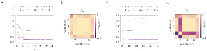
Fig. 6b illustrates an example where we jointly allocate two functional patterns for a complete graph with oscillators (see Supplementary Information for more details on this example).
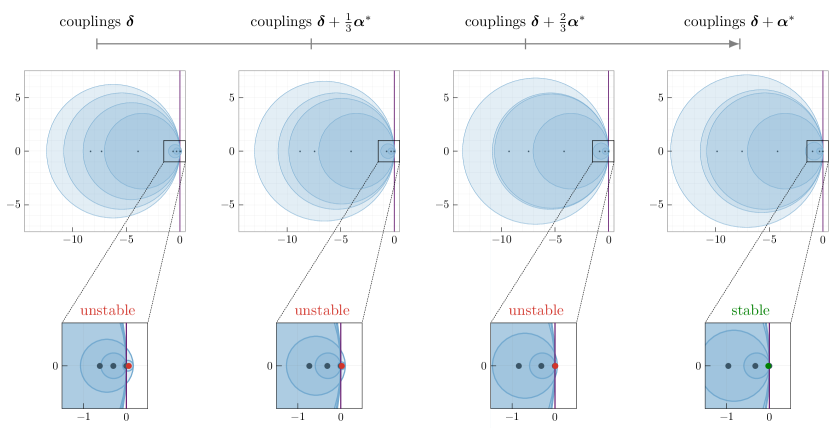
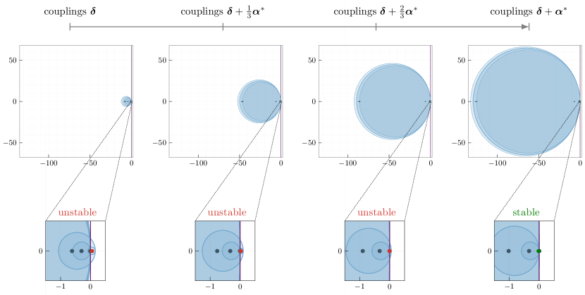
Note that the minimization problem (11) does not guarantee that the functional pattern is stable for the network with weights . To promote stability of the pattern , we use a heuristic procedure based on the classic Gerschgorin’s theorem [29]. Recall that stability of is guaranteed when the associated Jacobian matrix has a Laplacian structure, with negative diagonal entries and nonnegative off-diagonal entries. Further, instability of depends primarily on the negative off-diagonal entries of the Jacobian (these entries are negative because the sign of the network weight is different from the sign of the cosine of the desired phase difference ). Thus, reducing the magnitude of such entries heuristically moves the eigenvalues of the Jacobian towards the stable half of the complex plane (this phenomenon can be captured using the Gerschgorin circles, as we show in Fig. 7 for a network with nodes). To formalize this procedure, let and denote the entries of the weights and tuning vector , respectively, that are associated to negative interconnections in the cosine-scaled network. Then, the optimization problem that enacts the proposed strategy becomes:
| (13) | ||||
Carefully reducing the weights promotes stability of the target pattern. Fig. 7 illustrates the shift of the Jacobian’s eigenvalues while the optimal tuning vector is gradually applied to a -oscillator network to achieve stability of a functional pattern containing negative correlations (the network parameters can be found in the Supplementary Information). Finally, we remark that the procedure in (21) can be further refined by introducing scaling constants to penalize differently from the modification of other interconnection weights (see Supplementary Information for further details and an example).
The minimization problems (11) and (21) do not allow us to tune the oscillators’ natural frequencies, and are constrained to networks with positive weights. When any parameter of the network is unconstrained and can be adjusted to enforce a desired functional pattern, the network optimization problem can be generalized as
| (14) | ||||
| (14a) |
where denotes the correction to the natural frequencies. Problem (14) always admits a solution because can be chosen to satisfy the constraint (25a) for any choice of the network parameters . Further, the (unique) solution to the minimization problem (14) can also be computed in closed form:
where denotes the identity matrix.
We conclude this section by noting that the minimization problems (11)-(14) can be readily extended to include other vector norms besides the -norm in the cost function (e.g., the -norm to promote sparsity of the corrections), and to be applicable to directed networks. The latter extension can be attained by replacing the constraints (11a) and (25a) with a suitable rewriting of the matrix form (4). We refer the interested reader to the Supplementary Information for a comprehensive treatment of this extension and an example.
Applications to complex networks
In the remainder of this paper we apply our methods to an empirically reconstructed brain network and to the IEEE 39 New England power distribution network. In the former case, we use the Kuramoto model to map structure to function, and find that local metabolic changes underlie the emergence of functional patterns of recorded neural activity. In the latter case, we use our methods to restore the nominal network power flow after a fault.
Local metabolic changes govern the emergence of distinct functional patterns in the brain
The brain can be studied as a network system in which Kuramoto oscillators approximate the rhythmic activity of different brain regions [60, 59, 14, 45]. Over short time frames, the brain is capable of exhibiting a rich repertoire of functional patterns while the network structure and the interconnection weights remain unaltered. Functional patterns of brain activity not only underlie multiple cognitive processes, but can also be used as biomarkers for different psychiatric and neurological disorders [65].
To shed light on the structure-function relationship of the human brain, we utilize Kuramoto oscillators evolving on an empirically reconstructed brain network. We hypothesize that the intermittent emergence of diverse patterns stems from changes in the oscillators’ natural frequencies – which can be thought of as endogenous changes in metabolic regional activity regulated by glial cells [27] or exogenous interventions to modify undesired synchronization patterns [45]. First, we show that phase-locked trajectories of the Kuramoto model in equation (1) can be accurately extracted from noisy measurements of neural activity and are a relatively accurate approximation of neural activity.
We employ structural (i.e., interconnections between brain regions) and functional (i.e., time series of recorded neural activity) data from Ref. [60]. Structural connectivity consists of a sparse weighted matrix whose entries represent the strength of the physical interconnection between two brain regions. Functional data comprise time series of neural activity recorded through functional magnetic resonance imaging (fMRI) of healthy subjects as they rest. Because the phases of the measured activity have been shown to carry most of the information contained in the slow oscillations recorded through fMRI time series, we follow the steps in Ref. [60] to obtain such phases from the data by filtering the time series in the Hz frequency range (Supplementary Information). Next, since frequency synchronization is thought to be a crucial enabler of information exchange between different brain regions and homeostasis of brain dynamics [82, 53], we focus on functional patterns that arise from phase-locked trajectories, as compatible with our analysis. For simplicity, we restrict our study to the cingulo-opercular cognitive system, which, at the spatial scale of our data, comprises interacting brain regions [61].
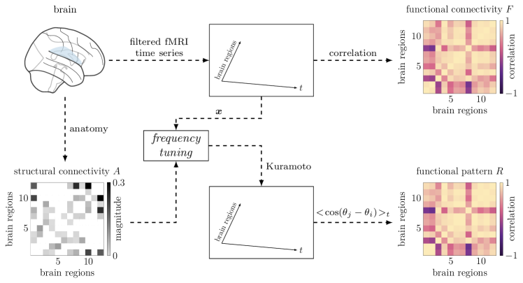
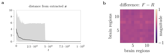
We identify time windows in the filtered fMRI time series where the signals are phase-locked, and compute two matrices for each time window: a matrix of Pearson correlation coefficients (also known as functional connectivity), and a functional pattern (as in equation (2)) from the phases extracted by solving the nonconvex phase synchronization problem [11]. Strikingly, we find that consistently (see Supplementary Information and Supplementary Figure 16b), thus demonstrating that our definition of functional pattern is a good replacement of the classical Pearson correlation arrangements in networks with oscillating states.
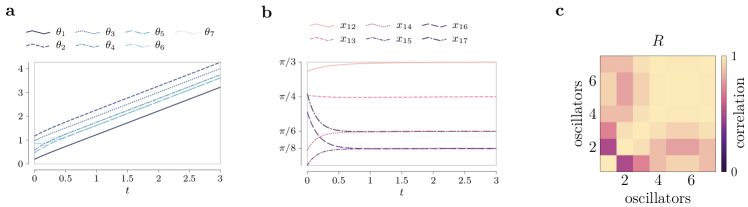
Building upon the above finding, we test whether the oscillators’ natural frequencies embody the parameter that links the brain network structure to its function (i.e., structural and functional matrices). We set , where are phase differences obtained from the previous step, and integrate the Kuramoto model in equation (1) with random initial conditions close to . We show in Fig. 8 that the assignment of natural frequencies according to the extracted phase differences promotes spontaneous synchronization to accurately replicate the empirical functional connectivity .
These results corroborate the postulate that structural connections in the brain support the intermittent activation of specific functional patterns during rest through regional metabolic changes. Furthermore, we show that the Kuramoto model represents an accurate and interpretable mapping between the brain anatomical organization and the functional patterns of frequency-synchronized neural co-fluctuations. Once a good mapping is inferred, it can be used to define a generative brain model to replicate in silico how the brain efficiently enacts large-scale integration of information, and to develop personalized intervention schemes for neurological disorders related to abnormal synchronization phenomena [83, 47].
Power flow control in power networks for fault recovery and prevention
Efficient and robust power delivery in electrical grids is crucial for the correct functioning of this critical infrastructure. Modern, reconfigurable power networks are expected to be resilient to distributed faults and malicious cyber-physical attacks [84] while being able to rapidly adapt to varying load demands. In addition, climate change is straining service reliability, as underscored by recent events such as the Texas grid collapse after Winter Storm Uri in February 2021 [13], and the New Orleans blackout after Hurricane Ida in August 2021 [1]. Therefore, there exists a dire need to design control methods to efficiently operate these networks and react to unforeseen disruptive events.
The Kuramoto model in equation (1) has been shown to be particularly relevant in the modeling of large distribution networks and microgrids [23]. Preliminary work on the control of frequency synchronization in electrical grids modeled through Kuramoto oscillators has been developed in Ref. [67]. Here, we present a method that leverages our findings to guarantee not only frequency synchronization, but also a target pattern of active power flow. Our method can be used for power (re)distribution with respect to specific pricing strategies, fault prevention (e.g., when a line overheats) and recovery (e.g., after the disconnection of a branch). Furthermore, thanks to the formal guarantees that our method prescribes, we are able to prevent Braess’ Paradox in power networks [85], which is a phenomenon where the addition of interconnections to a network may impede its synchronization.
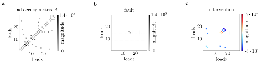
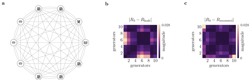
It has been shown in Ref. [23, Lemma 1] that the load dynamics (nodes - in Fig. 9a) in a structure-preserving power grid model have the same stable synchronization manifold of equation (1). In this model, is the active power load at node , where is the damping coefficient, and , with denoting the nodal voltage magnitude and being the imaginary part of the admittance (see Supplementary Information for details about this model). In this example, we choose a highly damped scenario where , which is possibly due to local excitation controllers. Notice that, when the phase angles are phase-locked and is fixed, the active power flow is given by .
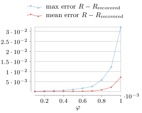
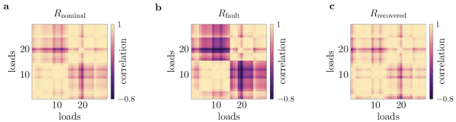
We posit that solving the problem in equation (11) to design a local reconfiguration of the network parameters can recover the power distribution before a line fault or provide the smallest parameter changes to steer the load powers to desired values. In practice, control devices such as Flexible Alternating Current Transmission Systems (FACTs) allow operators and engineers to change the network parameters [42, 50]. We demonstrate the effectiveness of our approach by recovering a desired power distribution in the IEEE 39 New England power distribution network after a fault. During a regime of normal operation, we simulate a fault by disconnecting the line between two loads and solve the problem in equation (11) to find the minimum modification of the couplings that recovers the nominal power distribution.
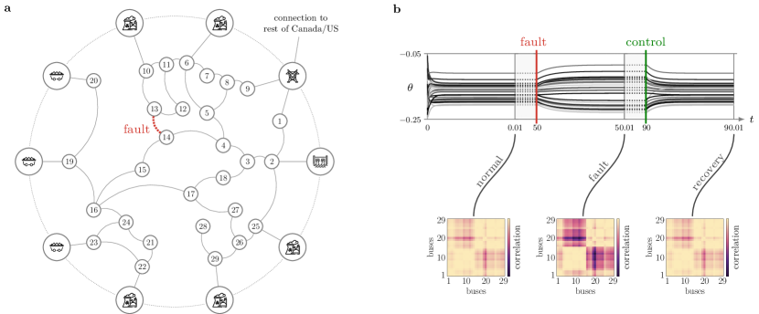
We first utilize MATPOWER [89] to solve the power flow problem. Then we use the active powers and voltages at the buses to obtain the natural frequencies and the adjacency matrix of the oscillators, respectively, while the voltage phase angles are used as initial conditions for the Kuramoto model in equation (1). We integrate the Kuramoto dynamics and let the voltage phases reach a frequency-synchronized steady state, which corresponds to a normal operating condition. The phase differences also represent a functional pattern across the loads. Next, to simulate a line fault, we disconnect one line. By solving the problem in equation (11) with corresponding to the pre-fault steady-state voltage phase differences, we compute the smallest variation of the remaining parameters (i.e., admittances) so that the original functional pattern can be recovered. Fig. 9b illustrates the effectiveness of our procedure at recovering the nominal pattern of active power flow by means of minimal and localized interventions (see also Supplementary Figure 17).
The above application is based on a classical lossless structure-preserving power network model [23]. However, in the power systems literature, more complex dynamics that relax some of the modeling assumptions have been proposed. For instance, Ref. [66] uses a third-order model (or one-axis model) that takes into account transient voltage dynamics. Instead, Ref. [33] studies the case of interconnections with power losses, which lead to a network of phase-lagged Kuramoto-Sakaguchi oscillators [63]. We show in the Supplementary Information that our procedure to recover a target functional pattern can still be applied successfully to a wide range of situations involving these more realistic models.
Contribution and future directions
Distinct configurations of synchrony govern the functioning of oscillatory network systems. This work presents a simple and mathematically grounded mapping between the structural parameters of arbitrary oscillator networks and their components’ functional interactions. The tantalizing idea of prescribing patterns in networks of oscillators has been investigated before, yet only partial results had been reported in the literature. Here, we demonstrate that the control of patterns of synchrony can be cast as optimal (convex) design and tuning problems. We also investigate the feasibility of such optimizations in the cases of networks that admit negative coupling weights and networks that are constrained to positive couplings. Our control framework also allows us to prescribe multiple desired equilibria in Kuramoto networks, a problem that is relevant in practice and had not been investigated before.
As stability of a functional pattern may be a compelling property in many applications, we explore conditions to test and enforce the stability of functional patterns. We show that such conditions are rather straightforward in the case of networks that admit both cooperative and competitive interactions. However, stability of target functional patterns in networks that are constrained to only cooperative interactions is a more challenging task, for which we demonstrate that any pattern associated to a structurally-balanced cosine-weighted network cannot be stable. To overcome this issue, we propose an heuristic procedure that adjusts the oscillators’ coupling strengths to violate the structurally-balanced property and promote the stability of functional patterns with negative correlations. While heuristic, our procedure for stability has proven successful in all our numerical studies. Notice that, differently from methods that study an “average” description of the system at near-synchronous state (see, e.g., Ref. [76]), here we assess the stability of exact target phase-locked trajectories where phase values can instead be arbitrarily spread over the torus. This method can also be extended to assess the stability of equilibria of higher-dimensional oscillators, provided that the considered equilibrium state is a fixed point.
We emphasize that our results are also intimately related to the long standing economic problem of enhancing network operations while optimizing wiring costs. In any complex system where synchrony between components ensures appropriate functions, it is beneficial to maximize synchronization while minimizing the physical variations of the interconnection weights [51]. Compatible with this principle, neural systems are thought to have evolved to maximize information processing by promoting synchronization through optimal spatial organization [3]. Inspired by the efficiency observed in neurobiological circuitry, equation (11) could be utilized for the design optimal interaction schemes in large-scale computer networks whose performance relies on synchronization-based tasks [41].
An important consideration that highlights the general contributions of the present study is that being able to specify pairwise functional relationships between the oscillators also solves problems such as phase-locking, full, and cluster synchronization. Yet, the converse is not true. In fact, even in the general setting of cluster synchronization [56] – where distinct groups of oscillators behave cohesively – one can only achieve a desired synchronization level within the same cluster, but not across clusters, which instead is possible with our approach. Specifically, in cluster-synchronization oscillators belonging to the same cluster are forced to synchronize, thus implying that the associated diagonal blocks of the functional pattern display values close to . Seminal work in Ref. [40] developed a nonlinear feedback control to change the coupling functions in equation (2) to engineer clusters of synchronized oscillators, whereas the authors of Ref. [24] propose the formation of clusters through selective addition of interconnections to the network. More recently, the control of partially synchronized states with applications to brain networks is studied in Ref. [45] by means of structural interventions, and in Ref. [8] via exogenous stimulation. Ultimately, the results presented in this work not only complement but go well beyond the control of macroscopic synchronization observables and partial synchronization by allowing to specify the synchrony level of pairwise interactions.
While our contributions include the analysis of the stability properties of functional patterns, here we do not assess their basins of attraction. We emphasize that, in general, the estimation of the basin of attraction of the attractors of nonlinear systems remains an outstanding problem, and even the most recent results rely on numerical approaches or heavy modeling assumptions [16]. Further, in the case of coupled Kuramoto oscillators, existing literature shows that the number of equilibria for the phase differences increases significantly with the cardinality of the network [44], making the study of basins of attraction extremely challenging. In the Supplementary Information, we extend previous work on identical oscillators to networks with heterogeneous oscillators, and show that that functional patterns can be at most almost-globally stable in cluster-synchronized positive networks. Yet, a precise estimation of the basin of attraction for any arbitrary target pattern goes beyond the scope of this work and may require the derivation of ad-hoc principles based on Lyapunov’s stability theory [88].
The framework presented in this work has other limitations, which can be addressed in follow up studies. First, despite its capabilities in modeling numerous oscillatory network systems, the Kuramoto model cannot capture the amplitude of the oscillations, making it most suitable for oscillator systems where most of the information is conveyed by phase interaction as demonstrated in Ref. [60] for resting brain activity. To model brain activity during cognitively demanding tasks such as learning, higher-dimensional oscillators may be more suitable [62]. Second, the use of phase-locked trajectories is instrumental to the control and design of functional patterns. Yet, it is not necessary. In fact, restricting the control to phase-locked dynamics does not capture exotic dynamical regimes in which only a subset of the oscillators is frequency-synchronized. Third and finally, in some situations the network parameters are not fully known. While being still an active area of research, network identification of oscillator systems may be employed in such scenarios [54].
Directions of future research can be both of a theoretical and practical nature. For instance, follow up studies can focus on the derivation of a general condition for the stability of a feasible functional pattern in positive networks. Further, a thorough investigation of which network structures allow for multiple prescribed equilibria may be particularly relevant in the context of memory systems, where different patterns are associated to different memory states. Specific practical applications may also require the inclusion of sparsity constraints on the accessible structural parameters for the implementation of the proposed control and design framework.
Methods
Matrix form of equation (1) and phase-locked solutions
For a given network of oscillators, we let the entries of the (oriented) incidence matrix be defined component-wise after choosing the orientation of each interconnection . In particular, points to if , and if oscillator is the source node of the interconnection , if oscillator is the sink node of the interconnection , and otherwise. The matrix form of equation (1) can be written as
where is the diagonal matrix of the sine functions in equation (1).
When the oscillators evolve in a phase-locked configuration, the oscillator frequencies become equal to each other and constant. In particular, since , we have , thus showing that, in any phase locked trajectory, the oscillators frequency needs to equal the mean natural frequency .
Any feasible functional pattern has degrees of freedom
The values of a functional pattern can be uniquely specified using a set of correlation values. To see this, let us define the incremental variables , where is the matrix whose -th row, associated to , is all zeros except for and . Consider the first rows of , associated to , and notice that they are linearly independent. Moreover, the row associated to , , can be obtained by subtracting the row associated to to the row associated to , implying that the rank of is . Any collection of linearly independent rows of defines a full row-rank matrix (e.g., any rows corresponding to the transpose incidence matrix of a spanning tree [30]). We let , where is a smallest set of phase differences that can be used to quantify the synchronization angles among all oscillators. Because , we can obtain the phases from modulo rotation: , where denotes the Moore-Penrose pseudo-inverse of and is some real number. Further, since , we can reconstruct all phase differences from :
The above equation reveals that all the differences are encoded in . That is, any can be written as a linear combination of the elements in . For example, if and , then is a linear combination of the differences in , i.e., , in which . Thus, because incremental variables define all the remaining ones, the entries of any functional pattern must have only degrees of freedom.
Existence of a strictly positive solution to Problem (5)
Rewrite the pattern assignment problem as
where the subscripts and denote the entries corresponding to the Hamiltonian path in conditions (ii.a)-(ii.b) and the remaining ones, respectively. Since , , and , for any vector , the following set of weights solves the above equation:
Because the matrix is an M-matrix, its inverse has nonnegative entries. Further, by condition (ii.b), is strictly positive. Then, the vector is also strictly positive, and so is the solution vector for any sufficiently small and positive vector .
Enforcing stability of functional patterns in networks with cooperative and competitive interactions
To ensure that the Jacobian matrix in equation (10) is the Laplacian of a positive network and, thus, stable, we solve the problem in equation (5) with a slight modification of the constraints. Specifically, we post-multiply the matrix in equation (5) as , where is a matrix that changes the sign of the columns of associated to negative weights in the cosine-scaled network:
Solving for positive interconnection weights the problem in equation (5) under the above modified constraint yields a stable Jacobian in a network where the final couplings are .
Heuristic procedure to promote stability of functional patterns in positive networks
We provide a heuristic procedure to promote the stability of functional patterns that include negative correlations in a network with nonnegative weights. Our procedure relies on the definition of Gerschgorin disks and the Gerschgorin Theorem.
Definition of Gerschgorin disk. Let be a complex matrix. The -th Gerschgorin disk is , , where the radius is and the center is .
Theorem 2
(Gerschgorin [29]). The eigenvalues of the matrix lie within the union of its Gerschgorin disks.
Whenever all target phase differences in satisfy , the Gerschgorin disks of the Jacobian in equation (10) all lie in the closed left half-plane. However, for patterns containing phase differences , the union of the Gerschgorin disks intersects the right half-plane. Reducing the magnitude of the entries satisfying effectively shrinks the radius of the Gerschgorin disks that overlap with the right half-plane and shifts their centers towards the left-half plane due to the structure of the Jacobian matrix. We remark that the procedure in equation (21) is a heuristic, and it is provably effective only when all interconnections with can be removed, so that all the Gerschgorin disks lie completely in the left-half plane.
Data availability
The brain data that support the findings of this study are available from the Supplementary Information of [60], https://doi.org/10.1371/journal.pcbi.1004100.s006. The IEEE 39 New England data parameters and interconnection scheme analyzed in this study for the structure-preserving power network model can be found in the reference textbook [64] (see also Supplementary Information for modeling assumptions). The parameters for the simulations on the network-reduced IEEE 39 New England test case in the Supplementary Information have been obtained from Ref. [77] and Ref. [48].
Code availability
Source code and documentation for the numerical simulations presented here are freely available in GitHub at: https://github.com/tommasomenara/functional_control with the identifier 10.5281/zenodo.4546413.
References
- [1] Hurricane Ida traps Louisianans, shatters the power grid. Associated Press, Aug 2021.
- [2] Juan A Acebrón, Luis L Bonilla, Conrad J Pérez Vicente, Félix Ritort, and Renato Spigler. The Kuramoto model: A simple paradigm for synchronization phenomena. Reviews of modern physics, 77(1):137, 2005.
- [3] S. Achard and E. Bullmore. Efficiency and cost of economical brain functional networks. PLOS Computational Biology, 3(2):e17, 2007.
- [4] A. Arenas, A. Díaz-Guilera, J. Kurths, Y. Moreno, and C. Zhou. Synchronization in complex networks. Physics Reports, 469(3):93–153, 2008.
- [5] A. Arenas, A. Díaz-Guilera, and C. J. Pérez-Vicente. Synchronization reveals topological scales in complex networks. Physical Review Letters, 96:114102, Mar 2006.
- [6] L. Arola-Fernández, A. Díaz-Guilera, and A. Arenas. Synchronization invariance under network structural transformations. Physical Review E, 97:060301, Jun 2018.
- [7] T. Athay, R. Podmore, and S. Virmani. A practical method for the direct analysis of transient stability. IEEE Transactions on Power Apparatus and Systems, 98(2):573–584, 1979.
- [8] K. Bansal, J. O. Garcia, S. H. Tompson, T. Verstynen, J. M. Vettel, and S. F. Muldoon. Cognitive chimera states in human brain networks. Science Advances, 5(4), 2019.
- [9] M. Beliaev, D. Zöllner, A. Pacureanu, P. Zaslansky, and I. Zlotnikov. Dynamics of topological defects and structural synchronization in a forming periodic tissue. Nature Physics, 2021.
- [10] I. Belykh, R. Jeter, and V. Belykh. Foot force models of crowd dynamics on a wobbly bridge. Science Advances, 3(11):e1701512, 2017.
- [11] N. Boumal. Nonconvex phase synchronization. SIAM Journal on Optimization, 26(4):2355–2377, 2016.
- [12] J. Buck and E. Buck. Biology of synchronous flashing of fireflies. Nature, 211(5049):562–564, 1966.
- [13] J. W. Busby, K. Baker, M. D. Bazilian, A. Q. Gilbert, E. Grubert, V. Rai, J. D. Rhodes, S. Shidore, C. A. Smith, and M. E. Webber. Cascading risks: Understanding the 2021 winter blackout in Texas. Energy Research & Social Science, 77:102106, 2021.
- [14] J. Cabral, E. Hugues, O. Sporns, and G. Deco. Role of local network oscillations in resting-state functional connectivity. NeuroImage, 57(1):130–139, 2011.
- [15] A. Cavagna, A. Cimarelli, I. Giardina, G. Parisi, R. Santagati, F. Stefanini, and M. Viale. Scale-free correlations in starling flocks. Proceedings of the National Academy of Sciences, 107(26):11865–11870, 2010.
- [16] S. Chen, M. Fazlyab, M. Morari, G. J. Pappas, and V. M. Preciado. Learning region of attraction for nonlinear systems. arXiv preprint arXiv:2110.00731, 2021.
- [17] M. C. Cross and P. C. Hohenberg. Pattern formation outside of equilibrium. Reviews of Modern Physics, 65(3):851, 1993.
- [18] A. Daffertshofer and B. van Wijk. On the influence of amplitude on the connectivity between phases. Frontiers in Neuroinformatics, 5:6, 2011.
- [19] G. Deco, J. Cruzat, J. Cabral, E. Tagliazucchi, H. Laufs, N. K. Logothetis, and M. L. Kringelbach. Awakening: Predicting external stimulation to force transitions between different brain states. Proceedings of the National Academy of Sciences, 116(36):18088–18097, 2019.
- [20] G. Deco, V. Jirsa, A. R. McIntosh, O. Sporns, and R. Kötter. Key role of coupling, delay, and noise in resting brain fluctuations. Proceedings of the National Academy of Sciences, 106(25):10302–10307, 2009.
- [21] F. Dörfler and F. Bullo. Synchronization and transient stability in power networks and nonuniform Kuramoto oscillators. SIAM Journal on Control and Optimization, 50(3):1616–1642, 2012.
- [22] F. Dörfler and F. Bullo. Synchronization in complex networks of phase oscillators: A survey. Automatica, 50(6):1539–1564, 2014.
- [23] F. Dörfler, M. Chertkov, and F. Bullo. Synchronization in complex oscillator networks and smart grids. Proceedings of the National Academy of Sciences, 110(6):2005–2010, 2013.
- [24] R. M. D’Souza and M. Mitzenmacher. Local cluster aggregation models of explosive percolation. Physical Review Letters, 104:195702, May 2010.
- [25] M. Fazlyab, F. Dörfler, and V. M. Preciado. Optimal network design for synchronization of coupled oscillators. Automatica, 84:181–189, 2017.
- [26] Juergen Fell and Nikolai Axmacher. The role of phase synchronization in memory processes. Nature Reviews Neuroscience, 12(2):105–118, 2011.
- [27] D. R. Fields, A. Araque, H. Johansen-Berg, S.-S. Lim, G. Lynch, K.-A. Nave, M. Nedergaard, R. Perez, T. Sejnowski, and H. Wake. Glial biology in learning and cognition. The Neuroscientist, 20(5):426–431, 2014.
- [28] A. Forrow, F. G. Woodhouse, and J. Dunkel. Functional control of network dynamics using designed Laplacian spectra. Physical Review X, 8(4):041043, 2018.
- [29] S. Geršgorin. Über die abgrenzung der eigenwerte einer matrix. Bulletin de l’Académie des Sciences de l’URSS. Classe des sciences mathématiques et na, pages 749–754, 1931.
- [30] C. Godsil and G. F. Royle. Algebraic Graph Theory. Graduate Texts in Mathematics. Springer New York, 2001.
- [31] Martin Golubitsky, Ian Stewart, and Andrei Török. Patterns of synchrony in coupled cell networks with multiple arrows. SIAM Journal on Applied Dynamical Systems, 4(1):78–100, 2005.
- [32] M. Grant, S. Boyd, and Y. Ye. CVX: Matlab software for disciplined convex programming, 2009.
- [33] F. Hellmann, P. Schultz, P. Jaros, R. Levchenko, T. Kapitaniak, J. Kurths, and Y. Maistrenko. Network-induced multistability through lossy coupling and exotic solitary states. Nature Communications, 11(1):592, 2020.
- [34] H. Hong and S. H. Strogatz. Kuramoto model of coupled oscillators with positive and negative coupling parameters: An example of conformist and contrarian oscillators. Physical Review Letters, 106(5):054102, 2011.
- [35] F. C. Hoppensteadt and E. M. Izhikevich. Weakly Connected Neural Networks. Springer, 1997.
- [36] R. A. Horn and C. R. Johnson. Matrix Analysis. Cambridge University Press, 1985.
- [37] P. Hövel, A. Viol, P. Loske, L. Merfort, and V. Vuksanović. Synchronization in functional networks of the human brain. Journal of Nonlinear Science, pages 1–24, 2018.
- [38] S. Kaka, M. R. Pufall, W. H. Rippard, T. J. Silva, S. E. Russek, and J. A. Katine. Mutual phase-locking of microwave spin torque nano-oscillators. Nature, 437(7057):389–392, 2005.
- [39] C. Kirst, M. Timme, and D. Battaglia. Dynamic information routing in complex networks. Nature Communications, 7(1):11061, 2016.
- [40] István Z. Kiss, Craig G. Rusin, Hiroshi Kori, and John L. Hudson. Engineering complex dynamical structures: Sequential patterns and desynchronization. Science, 316(5833):1886–1889, 2007.
- [41] G. Korniss, M. A. Novotny, H. Guclu, Z. Toroczkai, and P. A. Rikvold. Suppressing roughness of virtual times in parallel discrete-event simulations. Science, 299(5607):677–679, 2003.
- [42] A. L’Abbate, G. Migliavacca, U. Häger, C. Rehtanz, S. Rüberg, H. Ferreira, G. Fulli, and A. Purvins. The role of FACTS and HVDC in the future paneuropean transmission system development. In 9th IET International Conference on AC and DC Power Transmission (ACDC 2010), pages 1–8, 2010.
- [43] G. S. Medvedev and X. Tang. Stability of twisted states in the Kuramoto model on Cayley and random graphs. Journal of Nonlinear Science, 25(6):1169–1208, 2015.
- [44] D. Mehta, N. S. Daleo, F. Dörfler, and J. D. Hauenstein. Algebraic geometrization of the Kuramoto model: Equilibria and stability analysis. Chaos: An Interdisciplinary Journal of Nonlinear Science, 25(5):053103, 2015.
- [45] T. Menara, G. Baggio, D. S. Bassett, and F. Pasqualetti. A framework to control functional connectivity in the human brain. In IEEE Conf. on Decision and Control, pages 4697–4704, Nice, France, December 2019.
- [46] T. Menara, G. Baggio, D. S. Bassett, and F. Pasqualetti. Stability conditions for cluster synchronization in networks of heterogeneous Kuramoto oscillators. IEEE Transactions on Control of Network Systems, 7(1):302 – 314, 2020.
- [47] T. Menara, G. Lisi, F. Pasqualetti, and A. Cortese. Brain network dynamics fingerprints are resilient to data heterogeneity. Journal of Neural Engineering, 18(2):026004, 2021.
- [48] A. Moeini, I. Kamwa, P. Brunelle, and G. Sybille. Open data IEEE test systems implemented in SimPowerSystems for education and research in power grid dynamics and control. In 2015 50th International Universities Power Engineering Conference (UPEC), pages 1–6, 2015.
- [49] Joon-Young Moon, UnCheol Lee, Stefanie Blain-Moraes, and George A Mashour. General relationship of global topology, local dynamics, and directionality in large-scale brain networks. PLOS Computational Biology, 11(4):e1004225, 2015.
- [50] Adilson E Motter, Seth A Myers, Marian Anghel, and Takashi Nishikawa. Spontaneous synchrony in power-grid networks. Nature Physics, 9(3):191–197, 2013.
- [51] T. Nishikawa and A. E. Motter. Maximum performance at minimum cost in network synchronization. Physica D: Nonlinear Phenomena, 224(1-2):77–89, 2006.
- [52] T. Nishikawa and A. E. Motter. Network synchronization landscape reveals compensatory structures, quantization, and the positive effect of negative interactions. Proceedings of the National Academy of Sciences, 107(23):10342–10347, 2010.
- [53] R. Noori, D. Park, J. D. Griffiths, S. Bells, P. W. Frankland, D. Mabbott, and J. Lefebvre. Activity-dependent myelination: A glial mechanism of oscillatory self-organization in large-scale brain networks. Proceedings of the National Academy of Sciences, 117(24):13227–13237, 2020.
- [54] M. J. Panaggio, M. Ciocanel, L. Lazarus, C. M. Topaz, and B. Xu. Model reconstruction from temporal data for coupled oscillator networks. Chaos: An Interdisciplinary Journal of Nonlinear Science, 29(10):103116, 2019.
- [55] L. Papadopoulos, J. Z. Kim, J. Kurths, and D. S. Bassett. Development of structural correlations and synchronization from adaptive rewiring in networks of Kuramoto oscillators. Chaos: An Interdisciplinary Journal of Nonlinear Science, 27(7):073115, 2017.
- [56] L. M. Pecora, F. Sorrentino, A. M. Hagerstrom, T. E. Murphy, and R. Roy. Cluster synchronization and isolated desynchronization in complex networks with symmetries. Nature Communications, 5(1):1–8, 2014.
- [57] Louis M. Pecora and Thomas L. Carroll. Master stability functions for synchronized coupled systems. Physical Review Letters, 80:2109–2112, Mar 1998.
- [58] A. Pikovsky, M. Rosenblum, and J. Kurths. Synchronization: A Universal Concept in Nonlinear Sciences. Cambridge University Press, 2003.
- [59] A. Politi and M. Rosenblum. Equivalence of phase-oscillator and integrate-and-fire models. Physical Review E, 91(4):042916, 2015.
- [60] A. Ponce-Alvarez, G. Deco, P. Hagmann, G. L. Romani, D. Mantini, and M. Corbetta. Resting-state temporal synchronization networks emerge from connectivity topology and heterogeneity. PLoS Computational Biology, 11(2):1–23, 02 2015.
- [61] J. D. Power, A. L. Cohen, S. M. Nelson, G. S. Wig, K. A. Barnes, J. A. Church, A. C. Vogel, T. O. Laumann, F. M. Miezin, B. L. Schlaggar, and S. E. Petersen. Functional network organization of the human brain. Neuron, 72(4):665–678, 2011.
- [62] Y. Qin, T. Menara, D. S. Bassett, and F. Pasqualetti. Phase-amplitude coupling in neuronal oscillator networks. Physical Review Research, 3(2), June 2021.
- [63] H. Sakaguchi and Y. Kuramoto. A soluble active rotater model showing phase transitions via mutual entertainment. Progress of Theoretical Physics, 76(3):576–581, 1986.
- [64] P. W. Sauer and M. A. Pai. Power System Dynamics and Stability. Prentice Hall, 1998.
- [65] A. Schnitzler and J. Gross. Normal and pathological oscillatory communication in the brain. Nature Reviews Neuroscience, 6(4):285, 2005.
- [66] K. Sharafutdinov, L. Rydin Gorjão, M. Matthiae, T. Faulwasser, and D. Witthaut. Rotor-angle versus voltage instability in the third-order model for synchronous generators. Chaos: An Interdisciplinary Journal of Nonlinear Science, 28(3):033117, 2018.
- [67] P. S. Skardal and A. Arenas. Control of coupled oscillator networks with application to microgrid technologies. Science Advances, 1(7):e1500339, 2015.
- [68] P. S. Skardal and A. Arenas. Memory selection and information switching in oscillator networks with higher-order interactions. Journal of Physics: Complexity, 2(1):015003, dec 2020.
- [69] P. S. Skardal, D. Taylor, J. Sun, and A. Arenas. Collective frequency variation in network synchronization and reverse PageRank. Physical Review E, 93:042314, Apr 2016.
- [70] F. Sorrentino, M. Di Bernardo, and F. Garofalo. Synchronizability and synchronization dynamics of weighed and unweighed scale free networks with degree mixing. International Journal of Bifurcation and Chaos, 17(07):2419–2434, 2007.
- [71] F. Sorrentino and E. Ott. Network synchronization of groups. Physical Review E, 76(5):056114, 2007.
- [72] I. Stewart, M. Golubitsky, and M. Pivato. Symmetry groupoids and patterns of synchrony in coupled cell networks. SIAM Journal on Applied Dynamical Systems, 2(4):609–646, 2003.
- [73] S. H. Strogatz. Exploring complex networks. Nature, 410(6825):268–276, 2001.
- [74] S. H. Strogatz. SYNC: The Emerging Science of Spontaneous Order. Hyperion, 2003.
- [75] S. H. Strogatz and I. Stewart. Coupled oscillators and biological synchronization. Scientific American, 269(6):102–109, 1993.
- [76] J. Sun, E. M. Bollt, and T. Nishikawa. Master stability functions for coupled nearly identical dynamical systems. EPL (Europhysics Letters), 85(6):60011, 2009.
- [77] Y. Susuki, I. Mezić, and T. Hikihara. Coherent swing instability of power grids. Journal of nonlinear science, 21(3):403–439, 2011.
- [78] A. Townsend, M. Stillman, and S. H. Strogatz. Dense networks that do not synchronize and sparse ones that do. Chaos: An Interdisciplinary Journal of Nonlinear Science, 30(8):083142, 2020.
- [79] K. E. Trenberth. Spatial and temporal variations of the Southern Oscillation. Quarterly Journal of the Royal Meteorological Society, 102(433):639–653, 1976.
- [80] M. P. Van Den Heuvel and H. E. Hulshoff Pol. Exploring the brain network: a review on resting-state fmri functional connectivity. European Neuropsychopharmacology, 20(8):519–534, 2010.
- [81] M. van Wingerden, M. Vinck, J. Lankelma, and C. M. A. Pennartz. Theta-band phase locking of orbitofrontal neurons during reward expectancy. Journal of Neuroscience, 30(20):7078–7087, 2010.
- [82] F. Varela, J. P. Lachaux, E. Rodriguez, and J. Martinerie. The brainweb: Phase synchronization and large-scale integration. Nature Reviews Neuroscience, 2(4):229–239, 2001.
- [83] F. Váša, M. Shanahan, P. J. Hellyer, G. Scott, J. Cabral, and R. Leech. Effects of lesions on synchrony and metastability in cortical networks. Neuroimage, 118:456–467, 2015.
- [84] J.-W. Wang and L.-L. Rong. Cascade-based attack vulnerability on the US power grid. Safety Science, 47(10):1332 – 1336, 2009.
- [85] D. Witthaut and M. Timme. Braess’s paradox in oscillator networks, desynchronization and power outage. New Journal of Physics, 14(8):083036, aug 2012.
- [86] D. Zelazo and M. Bürger. On the robustness of uncertain consensus networks. IEEE Transactions on Control of Network Systems, 4(2):170–178, 2017.
- [87] F. Zhang and N. E. Leonard. Coordinated patterns of unit speed particles on a closed curve. Systems & Control Letters, 56(6):397–407, 2007.
- [88] L. Zhu and D. J. Hill. Synchronization of Kuramoto oscillators: A regional stability framework. IEEE Transactions on Automatic Control, 65(12):5070–5082, 2020.
- [89] R. D. Zimmerman, C. E. Murillo-Sánchez, and R. J. Thomas. MATPOWER: Steady-state operations, planning, and analysis tools for power systems research and education. IEEE Transactions on power systems, 26(1):12–19, 2010.
Supplementary Information
1 Supplementary Text
1.1 Comparison between our correlation metric and the Pearson correlation coefficient
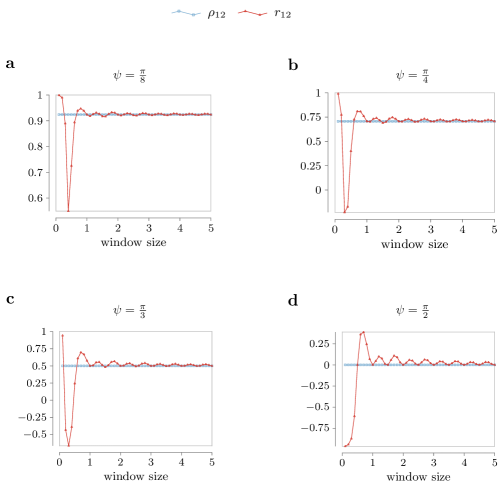
In this work, we provide methods and principles to guarantee the emergence of phase-locked trajectories that describe functional patterns. The latter are defined utilizing , instead of the classical Pearson correlation coefficient. The same metric is also utilized in [19] to quantify the similarity between BOLD signals in functional MRI recordings, and in [5], to quantify the synchrony in hierarchical networks.
To compare the two metrics, recall the definition of the classical (sample) Pearson correlation, which is a measure of linear correlation between two series of data, for vectors of samples and :
where and denote the sample means of vectors and , respectively. Notice that the length of the vectors and depends on the sampling time and on the window length. We argue that our metric (equation (2) in the main text) is simply more convenient when dealing with periodic phase signals. While we could use the Pearson correlation coefficient to define functional pattern instead of our cosine-based metric, the former does not perform well on periodic signals that evolve on the unit circle, and is heavily dependent on the time window employed to collect the samples. Thus, specific adjustments are needed to define correlation patterns through Pearson correlation coefficient for the class of time series (phase trajectories) studied in this work.
As an example, consider two identical sinusoidal signals (i.e., phase-locked) with natural frequency but shifted initial conditions: , , with . Fig. 10 illustrates the differences between the Pearson correlation coefficient and our correlation metric computed over a time window of varying length and for different values of the initial phase shift . In all panels, the values of vary at each point, emphasizing the dependence of the Pearson correlation coefficient from the length of the time window. Conversely, in all panels, the value of remains unaltered by the choice of time window length.
In conclusion, we choose to define functional patterns through because it is a convenient and suitable metric for this class of phase trajectories that naturally emerge in oscillator systems.
1.2 Stability results for functional patterns with angle differences larger than in the case of line and cycle with positive weights
Consider a line network of (ordered) oscillators with positive-only weights that possesses an equilibrium for the phase difference dynamics satisfying for some . It is straightforward to deduce from the results on structural balance [86] that the considered equilibrium is unstable. This implies that the functional pattern associated with that equilibrium is unstable.
Intuitively, the simplest topology that lends itself to a characterization of stable phase configurations including and allowing only positive weights is the cycle (i.e., a line network where the first and last oscillators are connected). Consider a cycle network of oscillators with positive weights, and denote with a vector of the phase differences between connected oscillators. We find that, after a suitable relabeling of the oscillators for which satisfies :
Theorem 2
(Stability of phase differences equilibria with in cycle networks) The equilibrium with , , and for all , is stable if and only if
-
(i)
for , with if , and ; -
(ii)
.
Moreover, if and , the largest possible value for such that is stable tends to the value , which is the solution to .
Proof of Theorem 2: To assess the stability of the equilibrium with , , and for all , we analyze the spectrum of the Jacobian . From Ref. [86, Corollary IV.7], we have that a necessary and sufficient condition for the Laplacian matrix of the cosine-scaled network to be positive semidefinite is
| (15) |
with being the effective resistance of the graph in which the edge has been removed. That is,
| (16) |
Since the adjacency matrix satisfies and is an equilibrium for the difference dynamics of the cycle network, the network weights must be identical pairwise:
| (17) |
for with the convention if . Thus, the angles being identical pairwise implies that the network weights must also be identical pairwise, which yields condition (i) of Theorem 2. Moreover, plugging the network weights from equation (17) into equation (16) yields
| (18) |
which makes the condition in Eq. (15) become, after algebraic calculations, condition (ii) of Theorem 2:
| (19) |
Thus, given that the Laplacian is positive definite, the Jacobian is stable, and its only zero eigenvalue is due to rotational symmetry of the right-hand side of the Kuramoto dynamics (equation (2) of the main manuscript).
1.3 Functional patterns possess at most almost-global stability in positive cluster-synchronized networks
In general, the analysis and estimation of the basin of attraction of nonlinear systems remains an outstanding problem, and even the most recent results rely on numerical approaches or heavy modeling assumptions [16]. To the best of our knowledge, Ref. [88] provides the most up-to-date study of the basins of attraction of synchronized Kuramoto oscillators. However, the authors in Ref. [88] only derive estimates of the basin of attraction for the fully synchronized case in networks of identical oscillators. Below, we show that functional patterns associated with phase-locked trajectories in cluster-synchronized positive networks are at most almost-globally stable. Our results extend previous work on identical oscillators to the case of oscillators with heterogeneous natural frequencies.
Existing literature shows that the number of equilibria for the phase differences of heterogeneous oscillators evolving on random graphs increases significantly with the cardinality of the network [44]. Therefore, we begin by restricting our analysis to the case of identical oscillators. In general, for any connected network of identical oscillators with cooperative connections , there is no unique pattern. In fact, the largest basin of attraction is achieved by -synchronizing graphs (e.g., complete graphs, acyclic graphs, and sufficiently dense graphs [22, 78]), which feature almost-global stability of the fully synchronized functional pattern. In this class of networks, the only stable equilibrium satisfies for all , and there exists a finite number of unstable equilibria. For instance, consider two connected identical oscillators: . The only stable equilibrium for the phase differences dynamics is . Yet, there also exists an unstable equilibrium . Note that, in general, almost-global stability cannot be guaranteed for arbitrary classes of sparse networks of identical oscillators, as other synchronization manifolds besides the fully synchronized one can be stable – for example, splay states emerge in Cayley graphs [43]. This latter class of graphs admits two stable equilibria (full synchronization and splay states), which implies the coexistence of two stable patterns.
We can generalize the above observations to networks of heterogeneous oscillators. To do so, we leverage cluster synchronization – a phenomenon where distinct groups of synchronized oscillators coexist in a network [46] – of -synchronizing clusters with possibly different natural frequencies. We consider cluster synchronization in networks with a partition of the oscillators , with being a subset of the network oscillators constituting an -synchronizing graph, , where and if . Further, for every , .111This is a necessary and sufficient condition for cluster synchronization [46]. Whenever cluster synchronization emerges, the diagonal blocks (of sizes , ) of the functional pattern associated with partition satisfy (see Supplementary Fig. 15).222Without loss of generality, we assume that the network oscillators are labeled such that consecutive labels belong to the same cluster. Thus, for a given number of clusters , each of the possible ways to partition the network yields a functional pattern with diagonal blocks corresponding to synchronized clusters.
By extending the above observations on the stability of -synchronizing graphs, we find that, in networks where at least one cluster satisfies , at most almost-global stability of cluster-synchronized functional patterns can be achieved. In fact, for any choice of intra-cluster phase differences from the finite set of unstable equilibria in -synchronizing graphs (i.e., for at least one intra-cluster phase difference), there exists a value for the inter-cluster phase differences for which the network admits phase-locked trajectories where intra-cluster phase differences satisfy or .
As an example, consider a -oscillator network partitioned as , where and . The network parameters read
Note that the two clusters are -synchronizing graphs. It can be shown that there exists an unstable equilibrium at . Thus, whenever the pattern associated to the partition is stable, it is at most almost-globally stable.
1.4 Allocation of multiple phase-locked equilibria by tailoring of the network structural parameters
The convex optimization problem proposed in the main text allows to tailor the network weights and the natural frequencies of the oscillators to specify multiple equilibria for the dynamics of the phase differences . These equilibria correspond to phase trajectories that evolve with constant, desired phase differences.
We now provide an example where we jointly impose, for a complete graph of oscillators, two equilibria for the phase difference dynamics. Specifically, by taking as a reference, we choose two points for the phase differences to be set as equilibria: and . The initial network parameters (adjacency matrix and zero-mean natural frequencies) read as:
respectively. To impose the desired equilibria, we numerically solve the following convex problem through standard cvx routines [32]:
| subject to |
The solution yields the following corrected adjacency matrix:
An investigation of the Jacobian spectrum (see main text for results on stability) of the phase differences computed at the two equilibria and reveals that the first equilibrium point is unstable and that the second one is locally stable. We illustrate the outcome of the above procedure to specify multiple equilibria in Fig. 6b in the main text, where the phase differences start at at time , and converge to after a perturbation is applied at to force them out from the equilibrium .
1.5 A heuristic method to promote stability of functional patterns in positive networks
To promote stability of functional patterns with phase differences , it is advantageous to design the network weights by minimizing the ones associated to a (i.e., reducing as much as possible) in the cosine-scaled network. Reducing the magnitude of these coupling strengths, or even pruning such interconnections, causes the Gerschgorin disks of the Laplacian to lie almost entirely in the right half-plane. In fact, by considering the limit case where all negative connections in the cosine-scaled network are pruned, if the remaining connections describe a connected network, then the Laplacian becomes a classical positive semi-definite Laplacian. This guarantees stability of the desired functional pattern and motivates the following heuristic procedure.
To showcase the effectiveness of the proposed heuristic method to promote stability, we construct an example with oscillators, interconnections, and desired minimum vector of phase differences
where , . Notice that the first difference , hence . Consider the oscillator network with structural parameters that read as:
| (20) |
Such a network admits the following phase-locked equilibrium
which differs from only in , and has all satisfying (thus generating a stable functional pattern). Supplementary Fig. 13a-b illustrate the stability of and the functional pattern associated with this equilibrium.
The network considered in this example has interconnections that can be modified, and the desired equilibrium implies that , so that is the modification of the first interconnection. To compute the optimal tuning of the network weights we solve the optimization (through standard cvx routines [32])
| (21) | ||||
The optimal reads
and the adjusted network adjacency matrix becomes:
| (22) |
where the optimal network correction has disconnected the entry (highlighted in red). The matrix guarantees stability of the functional pattern associated with , as we illustrate in Supplementary Fig. 13c-d.
In practice, one may jointly optimize the network weights to satisfy the equilibrium constraints and the heuristic stability strategy while trying to keep the overall modification as small as possible. To do so, we let (resp., ) denote the set of indices associated with (resp., ). Then, the optimization problem that enacts the proposed strategy reads as:
| (23) | ||||
where is a desired vector norm, are arbitrary penalty coefficients, denotes the entries of the tuning vector that are associated to positive weights in the cosine-scaled network, and denotes the entries of the tuning vector that are associated to negative weights in the cosine-scaled network.
To compute the optimal tuning of the network weights in the same -oscillator network above, we solve the optimization in Eq. (23) with and by minimizing the -norm. The optimal reads
and the adjusted network adjacency matrix becomes:
where, as in the procedure above, the optimal network correction has disconnected the entry (highlighted in red). Supplementary Fig. 14 illustrates the shift of the Jacobian’s eigenvalues while the optimal tuning vector is gradually applied. The main differences with respect to the minimization in (21) is that the norm of is smaller, and the eigenvalues of are closer to the original ones in .
1.6 Extension of the proposed optimization methods to directed networks
By relaxing the assumption on symmetric adjacency matrices, the matrix form of an oscillator network with Kuramoto dynamics in equation (3) of the main text does not hold anymore and requires a rewriting. In what follows, we use the subscript “” to indicate notation associated to directed graphs. Specifically, denote the oriented edge set, so that and denote the diagonal matrix of all with , and the vector of all the network weights , respectively. Further, let us define the modified incidence matrix whose columns have nonzero entries only at the edges’ sources. That is, if is the source of the interconnection , and otherwise. These definitions allow us to define the matrix form for a directed network of Kuramoto oscillators:
| (24) |
The main change in the behavior of directed networks with respect to undirected ones is that the frequencies of phase-locked trajectories do not typically converge to the average natural frequency (i.e., ). For phase-locked trajectories we have that , where the constant is not known a priori, and can only be estimated in the almost-fully synchronized regime for all [69]. Yet, not knowing as we do in the undirected case does not prevent the definition of a framework that can enforce a target functional pattern. In fact, by using equation (24) we can concurrently achieve the functional pattern associated with and assign a desired phase-locked frequency . To do so, we utilize equation (24) above with as a constraint in the optimization problems proposed in the main text. This modification allows us to extend any of the control methods to achieve desired functional relationships to directed networks.
As an example of optimization of the coupling strengths, we solve
| (25) | ||||
| (25a) |
for a network of oscillators with adjacency matrix and natural frequencies as follows:
where the entry highlighted in red is the one causing the asymmetry in the network coupling. The target phase differences are , and the desired phase locking frequency is rad/sec. The solution to problem (25) above yields
Supplementary Fig. 12 illustrates that the phase trajectories associated with such a solution achieve the target functional pattern.
We conclude this discussion by remarking that, besides our optimization problems, the sufficient conditions (i.a), (i.b), and (i.c) in the main text for the existence of positive coupling strengths that realize a target pattern can also be adapted to the case of directed networks. To show this, we let and . Then, a sufficient condition for the existence of positive network weights that achieve a desired functional pattern is the following one.
There exists such that if there exists a set satisfying:
-
(iii.a)
for all with ;
-
(iii.b)
for all ;
-
(iii.c)
.
Note that, since is not known a priori in most cases, these conditions are hard to check.
1.7 Coupled Kuramoto oscillators to approximate fMRI data
The interaction between static large-scale structural architecture of the human brain and local oscillations of neural communities is a key factor in the functional connectivity patterns that are empirically observed through functional magnetic resonance imaging (fMRI) when the brain is in a resting-state condition [80]. In the last two decades, extensive literature has resorted to Kuramoto phase oscillators to model fMRI data [20, 60, 59, 14, 83, 37, 45]. Many works, such as Ref. [60] and Ref. [14], focus on the analysis of the oscillatory behaviors of neural populations that lead the emergence of functionally connected networks by modeling fMRI data as the output of networks of Kuramoto oscillators. The main working assumption is that at each node of the structural brain network there exists a community of excitatory and inhibitory neurons whose dynamical state is in a regime of self-sustained oscillations. From a modeling standpoint, this assumption is equivalent to employing a network of weakly coupled Wilson-Cowan oscillators [35, 18], or to a supercritical Andronov-Hopf bifurcation, such as the Stuart-Landau model in oscillatory regime [49]. In this setting, the neurons’ firing rates describe a closed periodic trajectory in phase space; that is, the firing rates delineate a limit cycle. Thus, the dynamics can be approximated by a single variable, which is the angle (or phase) on this cycle. This regime is then modeled by a network of coupled heterogeneous Kuramoto oscillators that are connected to each other according to the architecture of the human brain.
1.8 Procedure to extract phase-locked trajectories from fMRI data
Following the procedure in Ref. [60], we apply a narrow-band filter in the low frequency range Hz to the time series for each brain region. Next, to obtain a measure of the functional synchrony between the brain regions, we generate the functional connectivity matrix , whose entry indicates the pairwise Pearson correlation coefficient between filtered time series of recorded neural activity. To map these functional correlations to the phase domain, we extracted the phase time series by applying a Hilbert Transform to the filtered signals. From , one can identify time windows over which frequency synchronization emerges with the aid of the phase-locking value matrix , where
Clearly, if for all , then the time window comprises phase-locked trajectories.
Since the phase time series are derived from inherently noisy measurements, we compute the best estimate of the phases (modulo rotation) that are compatible with the noisy measurement in by solving the nonconvex phase synchronization problem [11] – that is, the estimation of phases from noisy pairwise relative phase measurements. Given a time window of frequency-synchronized phase time series , we find that (see main text and Fig. 16). Moreover, it holds that as element-wise. This implies that functional relationships between the phases (encoded in the matrix ) represent the same functional relationships that are measured in fMRI data (encoded in the matrix ), supporting the usage of Kuramoto oscillators to analyze neural synchronization.
1.9 Power network modeling and assumptions
The main manuscript contains an application of our network tuning methods to the IEEE 39 New England power distribution network [7, 64]. To model the dynamics of this network, we consider a connected power network with generators and load buses . A structure-preserving power network model contains second-order Newtonian and first-order kinematic phase oscillators obeying [64]:
| (26) |
where , are the generator inertia constant, and the damping coefficient, respectively. In the equation for the generators , , which is the mechanical power input from the prime mover, and in the equation for the load buses , , which denotes the real power drawn by load . Finally, the weight equals , with denoting the nodal voltage magnitude and being the admittance matrix. The above structure-preserving power network model represents an AC grid with a synchronous generator.
Owing to Ref. [23, Lemma 1], the existence and local exponential stability of synchronized solutions of the oscillator model Eq. (26) can be entirely described by means of the first-order Kuramoto model. That is, the load dynamics of a structure-preserving power grid model has the same stable synchronization manifold of Eq. (1) in the main text.
We assume that thermal limit constraints are equivalent to phase cohesiveness requirements. To be precise, we obtain a bounded power flow for the line whenever the angular distance is bounded, which is satisfied by frequency-synchronized phase trajectories. Moreover, we assume constant voltage magnitudes at the loads, so that the weights can be considered fixed. This is a standard assumption in power systems ( also known as decoupling assumption). We refer the interested reader to Ref. [23, Remark 1] for further details.
The generators and bus parameters for the IEEE New England Power network are available in the original article and in classic textbooks [7, 64]. For simplicity, we set for all loads, which corresponds to a highly damped scenario, possibly due to local excitation controllers. In our simulations, we utilized the standard optimal power flow solver provided by MATPOWER to compute the parameters , and needed to integrate the Kuramoto model in Matlab through a standard ode45 solver.
1.10 Application to additional power network models
Depending on which assumptions are made and on which application is studied, there exist many different power network models in the literature. To demonstrate that the fundamental principles of our procedure remain unchanged even when dealing with more complex dynamics that relax some of the modeling assumptions, we apply our method to two models that differ from the one in equations (26). Henceforth, our goal is to intervene on a power network after a fault occurs between two loads in order to recover a desired (pre-fault) functional pattern.
First, we study the case of a third-order (also known as one-axis) model, such as the one in Ref. [66]. The main differences with the structure-preserving power network in equations (26) is that the model in Ref. [66] includes the transient dynamics of voltage magnitudes, and that electrical loads are simply modeled as passive impedances. For generators, Supplementary Fig. 18a illustrates the reduced power network model obeying the dynamics [66]
| (27) |
where is the rotor angle, its frequency, is the effective mechanical input power of the machine , and are the inertia and damping of the mechanical motion, respectively, indicates the transient voltage, is the susceptance of the transmission line , denotes the relaxation time of the transient voltage dynamics along the axis, is the internal voltage, and, finally, and are the static and transient reactances along the -axis.
Akin to the structure-preserving power network model, stationary operation of the grid corresponds to constant voltages and frequencies, along with constant rotor phase differences. Since our procedure relies on phase-locked trajectories to achieve a desired functional pattern (i.e., power flow), it can be adjusted to intervene on the stationary operation of a challenging model such as the one in equations (27). In fact, in regimes with small voltage and frequency swings, the system is still well approximated by first-order Kuramoto dynamics. Clearly, for a desired functional pattern, the error between the one estimated from the application of our procedure and the one obtained from the dynamics in equations (27) will be proportional to the changes in voltages and frequencies.
To test our approach on the model from equations (27), we use the same IEEE 39 New England benchmark case as in the main manuscript. The initial network parameters for our simulations, which represent standard grid operating conditions, are taken from Ref. [77] and Ref. [48]. The voltage and the initial condition for and for generator are fixed using power flow computation. The goal of this application is to recover the initial power flow after the same fault as in Ref. [77] (a line trip between loads 16 and 17) occurs. Such a fault affects the network admittance matrix, and yields an undesired power flow. To recover the pre-fault power flow we follow the same steps as described in the main text (see also Fig. 5b), but because the reduced-network structure is typically a complete graph [21], we do not modify its coupling strengths. Instead, we assume that we can adjust the values of , so that are the oscillators’ natural frequencies that are tuned in order to achieve the pre-fault functional patterns in the post-fault network. The values for are computed by rewriting the second one of equations (27) as equation (4) in the main text, and solving for the natural frequencies. For the coupling values in , we use , where denotes the steady state value of the voltage before applying our intervention. Finally, we sum a positive constant to the obtained natural frequencies so that they are all positive – this constant can be used to adjust the generators to a desired average mechanical input.
Supplementary Fig. 18b-c illustrate that our procedure is able to adequately recover the desired functional pattern after the line trips occurs. The error between the pre-fault pattern and the recovered one is due to small changes in the frequency and voltage values after is modified. We remark that our procedure relies on the dynamics of and leading to small changes. In situations where these changes significantly affect the phases dynamics, the first-order Kuramoto approximation leveraged by our method may not successfully recover a desired functional pattern.
We now turn our attention to models that do not neglect energy losses, such as the one in Ref. [33]. By compensating for the losses in the injected power but considering lossy interconnections, the structure-preserving model in equations (26) becomes,
| (28) |
where represents the phase shift induced by energy losses. We show in Fig. 19 that our procedure to restore a desired functional pattern in a lossy power network after a fault still works well for small values of the phase shift . We can recover functional patterns associated to target active power flow conditions by modifying the constraints of our optimization procedures to explicitly take into account the dynamics in equations (28).
At synchronous operating conditions, the dynamics in equations (28) reduce to the ones of Kuramoto-Sakaguchi oscillators [63]:
The phase shift makes the matrix formulation of the above dynamics to be incompatible with the ones we have introduced in equation (3) of the main text. We can instead write the above dynamics in matrix form by considering the graph as a directed graph (see also Supplementary Text 1.6 above), with being the set of directed edges. That is, we consider each undirected edge as two directed edges where each direction has the same weight . Then, we can write the following equation:
| (29) |
where satisfies if is the sink of the interconnection and otherwise, is the diagonal matrix of all , and is the synchronization frequency of phase-locked trajectories.
We are now ready to apply the equation (29) as a constraint in our numerical optimization routine. Without loss of generality, we set , and apply the same method developed for the lossless case to the IEEE 39 New England test case to compute the optimal correction after a fault occurs between loads 13 and 14 (the same as in the main text). For a loss , the updated optimization is able to recover the pre-fault functional pattern with a mean error , where vectorizes the matrix (see also Supplementary Fig. 20). This result improves upon the original method proposed for lossless networks by guaranteeing a satisfactory active power flow recovery for losses that are one order of magnitude larger. Finally, we observe that for the fixed parameters of this specific system cause the phases to lose frequency synchronization even at operating conditions.
2 Supplementary Figures