Functional Uniform Priors for Nonlinear Modelling

Suppose one would like to find a prior distribution for a parameter ${\boldsymbol{\theta}}$ in a compact subspace ${\boldsymbol{\Theta}}\subset\mathbb{R}^{p},\,p<\infty$. The approach proposed in this paper is to map the parameter ${\boldsymbol{\theta}}$ from ${\boldsymbol{\Theta}}$ into another compact metric space $(M,d)$, with metric $d$, using a differentiable bijective function $\varphi:{\boldsymbol{\Theta}}\mapsto M$, so that $\varphi({\boldsymbol{\theta}})={\boldsymbol{\phi}}\in M$. The metric $d$ should ideally define a reasonable measure of closeness and distance between the parameters, and its choice will of course be model and application dependent. In the exponential regression example, for instance, it seems adequate to measure the distance between two parameter values $\theta^{\prime}$ and $\theta^{\prime\prime}$ by a distance between the resulting functions $\exp(-x\theta^{\prime})$ and $\exp(-x\theta^{\prime\prime})$, rather than the Euclidean distance between the plain parameter values. In this metric space $(M,d)$, one then imposes a uniform distribution, reflecting the appropriate notion of distance of the metric space $(M,d)$, and transforms this distribution back to the parameter scale.

The construction of a uniform distribution in general metric spaces has been described by Dembski (1990), using the notion of packing numbers. Ghosal et al. (1997) apply this result for two particular Bayesian applications (derivation of Jeffreys prior for parametric problems and nonparametric density estimation). In the following we review and adapt this theory to our situation. Some basic mathematical notions are needed to present the ideas: Define an $\epsilon$-net as a set $S_{\epsilon}\subset M$, so that for all ${\boldsymbol{\phi}}^{\prime},{\boldsymbol{\phi}}^{\prime\prime}\in S_{\epsilon}$ holds $d({\boldsymbol{\phi}}^{\prime},{\boldsymbol{\phi}}^{\prime\prime})\geq\epsilon$, and the addition of any point to $S_{\epsilon}$ destroys this property. An $\epsilon$-lattice $S_{\epsilon}^{m}$ is the $\epsilon$-net with maximum possible cardinality. Dembski defines the uniform distribution on $M$ as the limit of a discrete uniform distribution on an $\epsilon$-lattice on $M$, when $\epsilon\rightarrow 0$.

Loosely speaking the uniform distribution is hence defined as the limit of a discrete uniform distribution on an equally spaced grid, where the notion of “equally spaced” is determined by the distance metric underlying $(M,d)$. Even though this definition is intuitive it is not constructive. Apart from special cases, generating an $\epsilon$-lattice is computationally difficult in a general metric space; calculating the limit of $\epsilon$-lattices even more so. In addition it is unclear, whether there is just one limit distribution all $\epsilon$-lattices would converge to. To overcome these problems Dembski (1990) uses the closely related notion of packing numbers. The packing number $D(\epsilon,A,d)$ of a subset $A\subset M$ in the metric $d$ is defined as the cardinality of an $\epsilon$-lattice on $A$, and packing numbers are known for a number of metric spaces. An $\epsilon$-pseudo-probability can then be defined as $P_{\epsilon}(A)=\frac{D(\epsilon,A,d)}{D(\epsilon,M,d)}$. It is straightforward to see that $0\leq P_{\epsilon}(A)\leq 1$ and that $P_{\epsilon}(M)=1$, but packing numbers are sub-additive and hence $P_{\epsilon}$ is not a probability measure. However for disjoint sets $A^{\prime}$ and $A^{\prime\prime}$ with minimum distance $>\epsilon$ additivity holds, i.e. $P_{\epsilon}(A^{\prime}\cup A^{\prime\prime})=P_{\epsilon}(A^{\prime})+P_{\epsilon}(A^{\prime\prime})$. Dembski (1990) then shows that whenever $\underset{\epsilon\rightarrow 0}{\lim}\,P_{\epsilon}(A)$ exists for any $A$, then the limit distribution is the unique uniform distribution on $(M,d)$ (see Dembski (1990) or Ghosal et al. (1997) for details). As packing numbers are known for a number of metric spaces, this result provides a constructive way for building uniform distributions, without the need for explicitly constructing $\epsilon$-lattices.

Subsequently we consider the practically important case of a finite number of parameters $p$ and assume that the metric of $(M,d)$, $d({\boldsymbol{\phi}},{\boldsymbol{\phi}}_{0})=d(\varphi({\boldsymbol{\theta}}),\varphi({\boldsymbol{\theta}}_{0}))=d^{*}({\boldsymbol{\theta}},{\boldsymbol{\theta}}_{0})$ in terms of ${\boldsymbol{\theta}}$ can be approximated by a local quadratic approximation of the form

where $c_{1},c_{2}>0$ are constants and $k\geq 3$. Equation (1) implies that $d(.,.)$ can locally be approximated by a Euclidean metric. This is not a very strong condition, for a sufficiently often differentiable metric $d(.,{\boldsymbol{\theta}}_{0})$ one can make use of a Taylor expansion of second order of $d(.,{\boldsymbol{\theta}}_{0})^{2}$ and apply the square root to obtain (1). The following theorem calculates the distribution induced on ${\boldsymbol{\theta}}$ by imposing a uniform distribution in $(M,d)$, when assumption (1) holds. The proof is only a slight adaption of earlier results by Ghosal et al. (1997), see Appendix A.

We note that the last result can be obtained as well by using considerations based on Riemannian manifolds, in which case (1) would be the Riemannian metric: For example Pennec (2006) explicitly considers uniform distributions on Riemannian manifolds and obtains the same result. We concentrated on Dembski’s derivation as it seems both more general and intuitive.

It is important to note that the so defined distribution is independent of the parametrization. This is intuitively clear, as the space $(M,d)$, where the uniform distribution is imposed, is fixed, no matter, which parametrization is used. We illustrate this invariance property for the special case of a Taylor approximation in the Theorem below; for a proof see Appendix B.

A technical restriction of the theory described in this section is the concentration on compact metric spaces ${\boldsymbol{\Theta}}$. However, it is possible to extend this based on taking limits of a sequence of growing compact spaces, see the works of Dembski (1990) and Ghosal et al. (1997) for details. Note that the resulting limiting density does not need to be integrable.

The implicit assumption when employing a nonlinear regression function $\mu(x,{\boldsymbol{\theta}})$, is that for one ${\boldsymbol{\theta}}$ the shape of the function $\mu(x,{\boldsymbol{\theta}})$ will adequately describe reality. It is usually unclear, however, which of these shapes is the right one. A uniform distribution on the functional shapes hence seems to be a reasonable prior. A suited metric space is consequently the space of functions $\mu(.,{\boldsymbol{\theta}})$, with $x\in\mathcal{X}\subset\mathbb{R}$, ${\boldsymbol{\theta}}\in K\subset\mathbb{R}^{p}$ with compact $K$ and metric for example given by the $L_{2}$ distance $d({\boldsymbol{\theta}},{\boldsymbol{\theta}}_{0})=\sqrt{\int_{\mathcal{X}}(\mu(x,{\boldsymbol{\theta}})-\mu(x,{\boldsymbol{\theta}}_{0}))^{2}dx}$. By a first order Taylor expansion one obtains $\mu(x,{\boldsymbol{\theta}})-\mu(x,{\boldsymbol{\theta}}_{0})=J_{x}({\boldsymbol{\theta}}_{0})({\boldsymbol{\theta}}-{\boldsymbol{\theta}}_{0})+O(||{\boldsymbol{\theta}}-{\boldsymbol{\theta}}_{0}||^{2})$, where $J_{x}({\boldsymbol{\theta}}_{0})=\frac{\partial}{\partial{\boldsymbol{\theta}}}\mu(x,{\boldsymbol{\theta}})$ is the row vector of first partial derivatives. This results in an approximation of form $(\mu(x,{\boldsymbol{\theta}})-\mu(x,{\boldsymbol{\theta}}_{0}))^{2}=({\boldsymbol{\theta}}-{\boldsymbol{\theta}}_{0})^{T}J_{x}({\boldsymbol{\theta}}_{0})^{T}J_{x}({\boldsymbol{\theta}}_{0})({\boldsymbol{\theta}}-{\boldsymbol{\theta}}_{0})+O(||{\boldsymbol{\theta}}-{\boldsymbol{\theta}}_{0}||^{3})$. Integrating this with respect to $x$ and taking the square root, leads to an approximation of $d({\boldsymbol{\theta}},{\boldsymbol{\theta}}_{0})$ of form $\sqrt{({\boldsymbol{\theta}}-{\boldsymbol{\theta}}_{0})^{T}{\boldsymbol{Z}}^{*}({\boldsymbol{\theta}}_{0})({\boldsymbol{\theta}}-{\boldsymbol{\theta}}_{0})+O(||{\boldsymbol{\theta}}-{\boldsymbol{\theta}}_{0}||^{3})},$ where ${\boldsymbol{Z}}^{*}({\boldsymbol{\theta}})=\int_{\mathcal{X}}J_{x}({\boldsymbol{\theta}})^{T}J_{x}({\boldsymbol{\theta}})dx$. Consequently, from Theorem 1 the functional uniform distribution for ${\boldsymbol{\theta}}$ equals $p({\boldsymbol{\theta}})\propto\sqrt{\det({\boldsymbol{Z}}^{*}({\boldsymbol{\theta}}))}.$ In the special case of a linear model $\mu(x,{\boldsymbol{\theta}})=f(x)^{T}{\boldsymbol{\theta}}$, the functional uniform distribution collapses to a constant prior distribution, which is the uniform distribution on ${\boldsymbol{\Theta}}$ for compact ${\boldsymbol{\Theta}}$ and improper, when extending to non-compact ${\boldsymbol{\Theta}}$.

We now revisit the exponential regression example from the introduction. In this case one obtains $J_{x}(\theta)=-x\exp(-\theta x)$, calculating $\int_{0}^{10}J_{x}(\theta)^{2}dx$ and applying the square root, one obtains $p(\theta)\propto\exp(-10\theta)\sqrt{\frac{\exp(20\theta)-200\theta^{2}-20\theta-1}{\theta^{3}}}$, normalizing this leads to the prior displayed in Figure 3 (i). On the $\theta$ scale the shape based functional uniform density hence leads to a rather non-uniform distribution. In Figure 3 (ii) one can observe that the probability mass is distributed uniformly over the different shapes, as desired.

An advantage of the functional uniform prior over the uniform prior is that it is independent of the choice of parameterization and not particularly sensitive to the potential choice of the bounds, provided all major shapes of the underlying function are covered. In Figure 3 (i) one can see that the density is already rather small at $\theta=5$ as most of the underlying functional shapes are already covered. In fact in this example one can extend the functional uniform distribution from the compact interval $[0,5]$ to a proper distribution on $[0,\infty)$.

Although the choice of the $L_{2}$ metric for $d$ seems reasonable in a variety of situations, other choices are possible. One could for example use a weighted version of the $L_{2}$ distance, when interest is in particular regions of the design space $\mathcal{X}$. In fact Jeffreys prior can be identified as a special case, when the assumed residual model is given by a homoscedastic normal distribution. In this situation the empirical measure on the design points is used as a weighting measure. The Jeffreys prior has also been mentioned by Bates and Watts (1988, p. 217), as a prior that is uniform on the response surfaces, but the possibility of an alternative weighting measures has not been considered.

One potential obstacle in the use of the proposed functional uniform prior is the fact that it can be computationally challenging to calculate. In some of the situations it might be possible to calculate ${\boldsymbol{Z}}^{*}({\boldsymbol{\theta}})$ analytically in others one might need to use numerical integration to approximate the underlying integrals. However, it needs to be noted that the prior only needs to be calculated once, as the prior is independent of the observed data (it only depends on the design region $\mathcal{X}$ and on potential parameter bounds), and can then be approximated for example in terms of more commonly used distributions. This approximation can then be reused in different modelling situations.

Here the IBScovars data set taken from the DoseFinding package will be used Bornkamp et al. (2010). The data were part of a dose ranging trial on a compound for the treatment of the irritable bowel syndrome with four active doses 1, 2, 3, 4 equally distributed in the dose range $[0,4]$ and placebo. The primary endpoint was a baseline adjusted abdominal pain score with larger values corresponding to a better treatment effect. In total 369 patients completed the study, with nearly balanced allocation across the doses. Assume a normal distribution is used to model the residual error and that the hyperbolic Emax model $\mu(x,{\boldsymbol{\theta}})=\theta_{0}+\theta_{1}x/(\theta_{2}+x)$ was chosen to describe the dose-response relationship. The parameters $\theta_{0}$ and $\theta_{1}$ determine the placebo mean and the asymptotic maximum effect, while the parameter $\theta_{2}$ determines the dose that gives 50 percent of the asymptotic maximum effect, so that it determines the steepness of the curve. In clinical practice vague prior information typically exists for $\theta_{0}$ and $\theta_{1}$, but for illustration here we use improper constant priors for these two parameters and a prior proportional to $\sigma^{-2}$ for $\sigma$. For the nonlinear parameter $\theta_{2}$ we will use a uniform prior and the functional uniform prior distribution. When using a uniform distribution for $\theta_{2}$ it is necessary to assume bounds, as otherwise an improper posterior distribution may arise. We will use the bounds $[0.004,6]$ here, the selection of the boundaries is based on the fact that practically all of the shapes of the underlying model are covered taking into account that the dose range is $[0,4]$. For comparability for the functional uniform prior the same bounds were used, although one can extend it to an integrable density on $[0,\infty)$. The functional uniform prior will be used based on the function space defined by $x/(\theta_{2}+x)$. Performing the calculations described in Section 2.2 one obtains $J^{2}_{x}={{x^{2}}/{\left(x+\theta_{2}\right)^{4}}}$, calculating the integral $\int_{0}^{4}J^{2}_{x}(\theta_{2})\,dx$ and applying the square root leads to $p(\theta_{2})\propto{1}/{\sqrt{\theta_{2}^{4}+12\theta_{2}^{3}+48\theta_{2}^{2}+64\theta_{2}}}1_{[0.004,6]}(\theta_{2})$. Similar to the exponential regression example in the introduction, a uniform distribution on $\theta_{2}$ space induces an informative distribution in the space of functional shapes. Shapes corresponding to larger values of $\theta_{2}$ (say $>3$) correspond to almost linear shapes, while only very small values of $\theta_{2}$ lead to more pronounced concave shapes. A uniform prior on $\theta_{2}$ hence induces a prior that favors linear shapes over steeply increasing model shapes.

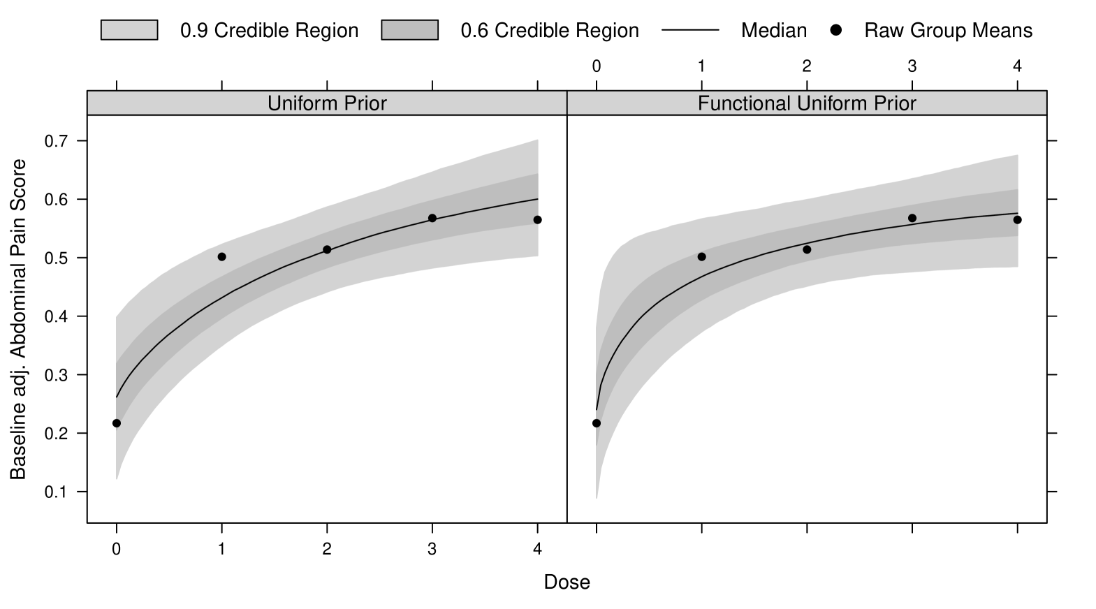
We used importance sampling resampling based on a proposal distribution generated by the iterated Laplace approximation to implement the model (see, Bornkamp (2011)). In Figure 4 one can observe the posterior uncertainty intervals under the two prior distributions. As is visible, the bias towards linear shapes, when using a uniform distribution for $\theta_{2}$ pertains in the posterior distribution. This happens despite the rather large sample size, and despite the fact that the response at the doses 0, 4 and particularly at dose 1 are not very well fitted by a linear shape. So the posterior seems to be rather sensitive to the prior uniform distribution. The posterior based on the shape based functional uniform prior, in contrast, fits the data better at all doses, and seems to provide a more realistic measure of uncertainty for the dose-response curve, particularly for $x\in(0,1)$.

One might expect that the functional uniform prior distribution works acceptable no matter which functional shape is the true one. To investigate this in more detail and to compare this prior to other prior distributions in terms of their frequentist performance, simulation studies have been conducted. Here we report results from simulations in the context of binary nonlinear regression.

For simulation the power model $\mu(x,\theta)=\theta_{0}+\theta_{1}x^{\theta_{2}}$ will be used to model the response probability depending on $x$. The parameters $\theta_{0}$ and $\theta_{1}$ are hence subject to $\theta_{0}+\theta_{1}\leq 1$ and $\theta_{0},\theta_{1}\geq 0$, as a probability is modelled. Note that only $\theta_{2}$ enters the model function non-linearly

The doses $0,0.05,0.2,0.6,1$ are to be used with equal allocations of 20 patients per dose. We use four scenarios in this case: in the first three cases the power model is used with $\theta_{0}=0.2$ and $\theta_{1}=0.6$, while $\theta_{2}$ is equal to $0.4$ (Power 1), $1$ (Linear) and $4$ (Power 2). In addition we provide one scenario, where an Emax model $0.2+0.6/(x+0.05)$ is the truth. The Emax scenario is added to investigate the behaviour under misspecification of the model. Each simulation scenario will be repeated 1000 times.

We will compare the functional uniform prior distribution to the uniform distribution on the parameters and to the Jeffreys prior distribution. For the uniform prior distribution approach uniform prior distributions were assumed for all parameters, and the nonlinear parameter $\theta_{2}$ was assumed to be within $[0.05,20]$ to ensure integrability. The same bounds are used for the two other approaches for comparability. For the functional uniform prior approach, uniform priors are used for $\theta_{0}$ and $\theta_{1}$, while for $\theta_{2}$ the functional uniform prior will be used on the function space defined by $x^{\theta_{2}}$. The prior can be calculated to be $p(\theta_{2})\propto 1/\sqrt{2\theta_{2}^{3}/3+\theta_{2}^{2}+\theta_{2}/2+1}$. For the Jeffreys prior approach we used a prior proportional to $\sqrt{{\det(I({\boldsymbol{\theta}}))}}$, within the imposed parameter bounds. For analysis we used MCMC based on the HITRO algorithm, which is an MCMC sampler that combines the hit and run algorithm with the ratio of uniforms transformation. It does not need tuning and is hence well suited for a simulation study. The sampler is implemented in the Runuran package (Leydold and Hörmann, 2010), computations were performed with R (R Development Core Team, 2011). 10000 MCMC samples are used from the corresponding posterior distributions in each case, using a burnin phase of 1000 a thinning of 2.

In Table 1 one can observe the estimation results in terms of the mean absolute estimation error for the dose-response function, $\mathrm{MAE}=1/9\sum_{i=0}^{8}|\mu(i/8)-\hat{\mu}(i/8)|$, where $\mu(.)$ is the underlying true function and $\hat{\mu}(.)$ is either the point wise posterior median (corresponding to MAE₁) or the prediction corresponding to the posterior mode for the parameters (MAE₂), the posterior mode for the uniform prior is equal to the maximum likelihood estimate. The values displayed in Table 1 are the average $\mathrm{MAE}$ over 1000 repetitions. In addition for each simulation the 0.9 credibility intervals at the dose-levels $0,1/8,2/8,...,1$ have been calculated. The number given in the Table is $CP=1/9\sum_{i=0}^{8}\hat{P}_{i/8}$, where $\hat{P}_{d}$ is the average coverage probability of the 0.9 credibility interval at dose $d$ over 1000 simulation runs. In addition the average length of the credibility intervals has been calculated as $ILE=1/9\sum_{i=0}^{8}\hat{L}_{i/8}$, where $L_{d}$ is the average length of the 0.9 credibility interval at dose $d$ over 1000 simulation runs. For estimation of the dose-response Jeffreys prior and the functional uniform prior improve upon the uniform prior distribution, while the Jeffreys prior and the functional uniform prior are close, with slight advantages for the Jeffreys prior. In terms of the credibility intervals the functional uniform and Jeffreys prior roughly keep their nominal level for the linear, and the power model cases, while the uniform prior probability does not. None of the priors achieves the nominal level for the Emax model, which is probably due to the fact that the Emax model is too different from the power model. Interestingly the credibility intervals of the uniform prior are larger than those of the other two priors, but lead to a smaller coverage probability.

Table 2 provides the estimation results with respect to parameter estimation. The main message here is that all priors perform roughly equal for estimation of the linear parameters $\theta_{0}$ and $\theta_{1}$. For the nonlinear parameters, Jeffreys prior distribution and the functional uniform prior perform better than the uniform disribution.

In summary the functional uniform prior hence performs roughly equally well as the Jeffreys prior in these simulations. However, the functional uniform prior has the pragmatic and conceptual advantages that it does not depend on the observed covariates, and can thus be used for example for calculation of a Bayesian optimal design, or in sequential situations.

In this section we will use the prior distribution for the exponential regression model derived in Section 2.2 to calculate a Bayesian optimal design. When assuming a homoscedastic normal model, the Fisher information is $I(d,\theta)\propto\sum w_{i}x_{i}^{2}\exp(-2\theta x_{i})$. Hence minimizing $-\log(I(d,\theta))$ will lead to a design with most information. Unfortunately the expression depends on $\theta$, which is of course unknown before the experiment. One way of dealing with this uncertainty are Bayesian optimal designs, where one optimizes the design criterion averaged with respect to a prior distribution: $-\int\log(I(d,\theta))p(\theta)d\theta$. In this situation we will use the uniform and functional uniform prior distribution (see Figures 1 and 3) both on the interval $[0,5]$ for calculation of the optimal design. Restricting the design space to $x\in[0,10]$ and only performing the optimization up to 5 design points, one ends up with the weights ${\boldsymbol{w}}=(0.956,0.022,0.022)$ on the design points $x=(0.38,4.04,10)$, for the uniform prior, while the functional uniform prior distribution leads to a design of the form ${\boldsymbol{w}}=(0.19,0.3,0.51)$ and $x=(0.54,2.35,10)$. The design corresponding to the functional uniform prior hence spreads its allocation weights more uniformly on the design range, whereas the uniform prior results in essentially one major design point.

One way of comparing the two calculated designs is to look at the efficiency $\mathrm{Eff}(d,\theta)=\exp(\log(I(d,\theta))-\log(I(d_{opt}(\theta),\theta)))$, of the calculated designs, with respect to the design $d_{opt}(\theta)$ that is locally optimal for the parameter value $\theta$, for a range of different shapes. In Figure 5 we plot the efficiency for the different shapes on the functional shape scale.

One can observe that the uniform prior design is only efficient for the sharply decreasing shapes with $\theta>0.71$, but otherwise has very low efficiency. The functional uniform prior improves quite a bit over the uniform prior distribution for most of the functional shape space, and provides at least a reasonable efficiency for most shapes.

References

- Balasubramanian (1997) Balasubramanian, V. (1997). Statistical inference, Occam’s razor, and statistical mechanics on the space of probability distributions. Neural Computation 9, 349–369.
- Bates and Watts (1988) Bates, D. M. and Watts, D. G. (1988). Nonlinear Regression Analysis and Applications. John Wiley and sons, New York.
- Berger et al. (2009) Berger, J. O., Bernardo, J. M., and Sun, D. (2009). The formal definition of reference priors. Annals of Statistics 37, 905–938.
- Bornkamp (2011) Bornkamp, B. (2011). Approximating probability densities by iterated Laplace approximations. Journal of Computational and Graphical Statistics 00, 00–00.
- Bornkamp and Ickstadt (2009) Bornkamp, B. and Ickstadt, K. (2009). A note on B-splines for semiparametric elicitation. The American Statistician 63, 373–377.
- Bornkamp et al. (2010) Bornkamp, B., Pinheiro, J., and Bretz, F. (2010). DoseFinding: Planning and Analyzing Dose Finding experiments. R package version 0.4-1.
- Daniels (1999) Daniels, M. J. (1999). A prior for the variance in hierarchical models. Canadian Journal of Statistics 27, 567–578.
- Dembski (1990) Dembski, W. A. (1990). Uniform probability. Journal of Theoretical Probability 3, 611–626.
- Dragalin et al. (2010) Dragalin, V., Bornkamp, B., Bretz, F., Miller, F., Padmanabhan, S. K., Patel, N., Perevozskaya, I., Pinheiro, J., and Smith, J. R. (2010). A simulation study to compare new adaptive dose-ranging designs. Statistics in Biopharmaceutical Research 2, 487–512.
- Dryden et al. (2009) Dryden, I. L., Koloydenko, A., and Zhou, D. (2009). Non-Euclidean statistics for covariance matrices with applications to diffusion tensor imaging. Annals of Applied Statistics 3, 1102–1123.
- Ghosal et al. (1997) Ghosal, S., Ghosh, J. K., and Ramamoorthi, R. V. (1997). Non-informative priors via sieves and packing numbers. In Panchapakesan, S. and Balakrishnan, N., editors, Advances in Statistical Decision Theory and Applications, pages 119–132. Birkhäuser, Boston.
- Ghosh et al. (2006) Ghosh, J. K., Delampady, M., and Samanta, T. (2006). An Introduction to Bayesian Analysis: Theory and Methods. Springer, New York.
- Jeffreys (1961) Jeffreys, H. (1961). Theory of Probability. Oxford University Press.
- Jones et al. (2010) Jones, D. S., Plank, M. J., and Sleeman, B. D. (2010). Differential Equations and Mathematical Biology. Chapman and Hall, Boca Raton.
- Kass and Wasserman (1996) Kass, R. E. and Wasserman, L. (1996). The selection of prior distributions by formal rules. Journal of the American Statistical Association 91, 1343–1370.
- Kolmogorov and Tihomirov (1961) Kolmogorov, A. N. and Tihomirov, V. M. (1961). entropy and capacity of sets in function spaces. American Mathematics Society Translations Ser. 2 17, 277–364.
- Leydold and Hörmann (2010) Leydold, J. and Hörmann, W. (2010). Runuran: R interface to the UNU.RAN random variate generators. R package version 0.15.0.
- Lindsey (2001) Lindsey, J. K. (2001). Nonlinear Models for Medical Statistics. Oxford University Press, Oxford.
- Müller et al. (2006) Müller, P., Berry, D. A., Grieve, A. P., and Krams, M. (2006). A Bayesian decision-theoretic dose-finding trial. Decision Analysis 3, 197–207.
- Neuenschwander et al. (2010) Neuenschwander, B., Capkun-Niggli, G., Branson, M., and Spiegelhalter, D. J. (2010). Summarizing historical information on controls in clinical trials. Clinical Trials 7, 5–18.
- O’Hagan et al. (2006) O’Hagan, A., Buck, C., Daneshkhah, A., Eiser, R., Garthwaite, P., Jenkinson, D., Oakley, J., and Rakow, T. (2006). Uncertain Judgements: Eliciting Expert Probabilities. John Wiley and Sons Inc.
- O’Hagan and Forster (2004) O’Hagan, A. and Forster, J. (2004). Kendall’s Advanced Theory of Statistics, Volume 2B: Bayesian Inference. Arnold, London, 2nd edition.
- Paulo (2005) Paulo, R. (2005). Default priors for Gaussian processes. Annals of Statistics 33, 556–582.
- Pennec (2006) Pennec, X. (2006). Intrinsic statistics on Riemannian manifolds: Basic tools for geometric measurements. Journal of Mathematical Imaging and Vision 25, 127–154.
- R Development Core Team (2011) R Development Core Team (2011). R: A Language and Environment for Statistical Computing. R Foundation for Statistical Computing, Vienna, Austria. ISBN 3-900051-07-0.