Fundamental limits to learning closed-form mathematical models from data

The complete probabilistic solution to the problem of identifying a model from observations is encapsulated in the posterior distribution over models $p(m|D)$. The posterior gives the probability that each model $m=m(\mathbf{x},\theta)$, with parameters $\theta$, is the true generating model given the data $D$. Again, notice that we are interested on the posterior over model structures $m$ rather than model parameters $\theta$; thus, we obtain $p(m|D)$ by marginalizing $p(m,\theta|D)$ over possible parameter values $\Theta$

where $p(D|m,\theta)$ is the model likelihood, and $p(\theta|m)$ and $p(m)$ are the prior distributions over the parameters of a given model and the models themselves, respectively. The posterior over models can always be rewritten as

with $Z=p(D)=\sum_{\{m\}}\exp\left[-\mathcal{H}(m)\right]$ and

Although the integral over parameters in Eq. (Probabilistic formulation of the problem) cannot, in general, be calculated exactly, it can be approximated as Schwarz (1978); Guimerà et al. (2020)

where $B(m)$ is the Bayesian information criterion (BIC) of the model Schwarz (1978). This approximation results from using Laplace’s method integrate the distribution $p(D|m,\theta)p(\theta|m)$ over the parameters $\theta$. Thus, the calculation assumes that: (i) the likelihood $p(D|m,\theta)$ is peaked around $\theta^{*}=\arg\max_{\theta}p(D|m,\theta)$, so that it can be approximated by a Gaussian around $\theta^{*}$; (ii) the prior $p(\theta|m)$ is smooth around $\theta^{*}$ so that it can be assumed to be approximately constant within the Gaussian. Unlike other contexts, in regression-like problems these assumptions are typically mild.

Within an information-theoretical interpretation of model selection, $\mathcal{H}(m)$ is the description length, that is, the number of nats (or bits if one uses base 2 logarithms instead of natural logarithms) necessary to jointly encode the data and the model with an optimal encoding Grünwald (2007). Therefore, the most plausible model—that is, the model with maximum $p(m|D)$—has the minimum description length, that is, compresses the data optimally.

The posterior in Eq. (2) can also be interpreted as in the canonical ensemble in statistical mechanics, with $\mathcal{H}(m)$ playing the role of the energy of a physical system, models playing the role of configurations of the system, and the most plausible model corresponding to the ground state. Here, we sample the posterior distribution over models $p(m|D)$ by generating a Markov chain with the Metropolis algorithm, as one would do for physical systems. To do this, we use the “Bayesian machine scientist” introduced in Ref. Guimerà et al. (2020) (Methods). We then select, among the sampled models, the most plausible one (that is, the maximum a posteriori model, the minimum description length model, or the ground state, in each interpretation).

Probabilistic model selection as described above follows directly (and exactly, except for the explicit approximation in Eq. (4)) from the postulates of Cox’s theorem Cox (1946); Jaynes (2003) and is therefore (Bayes) optimal when models are truly drawn from the prior $p(m)$. In particular, the minimum description length (MDL) model is the most compressive and the most plausible one, and any approach selecting, from $D$, a model that is not the MDL model violates those basic postulates.

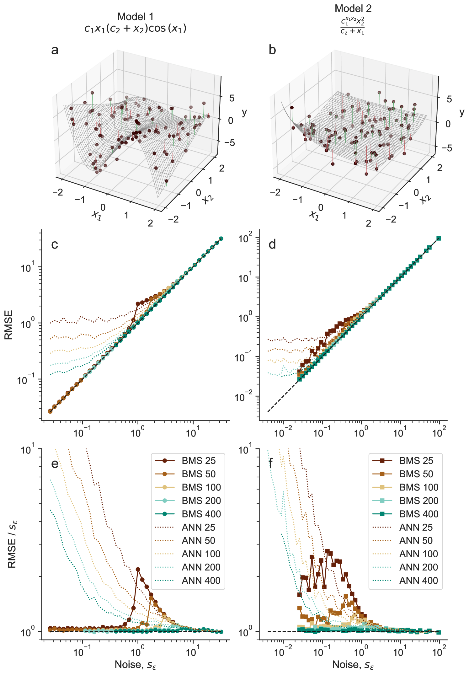
We start by investigating whether this optimality in model selection also leads to the ability of the MDL model to generalize well, that is, to make accurate predictions about unobserved data. We show that the MDL model yields quasi-optimal generalization despite the fact that the best possible generalization is achieved by averaging over models Guimerà et al. (2020), and despite the BIC approximation in the calculation of the description length (Fig. 1). Specifically, we sample a model $m^{*}$ from the prior $p(m)$ described in Ref. Guimerà et al. (2020) and in the Methods; for a model not drawn from the prior, see Supplementary Text and Fig. S1. From this model, we generate synthetic datasets $D=\left\{(y_{i},\mathbf{x}_{i})\right\}$, $i=1,\dots,N$ (where $y_{i}=m^{*}(\mathbf{x}_{i},{\theta^{*}})+\epsilon_{i}$ and $\epsilon_{i}\sim{\rm Gaussian}(0,s_{\epsilon})$) with different number of points $N$ and different levels of noise $s_{\epsilon}$. Then, for each dataset $D$, we sample models from $p(m|D)$ using the Bayesian machine scientist Guimerà et al. (2020), select the MDL model among those sampled, and use it to make predictions on a test dataset $D^{\prime}$.

Because $D^{\prime}$ is, like $D$, subject to observation noise, the irreducible error is $s_{\epsilon}$, that is, the root mean squared error (RMSE) of predictions cannot be, on average, smaller than $s_{\epsilon}$. As we show in Fig. 1, the predictions of the MDL model achieve this optimal prediction limit except for small $N$ and some intermediate values of the observation noise. This is in contrast to standard machine learning algorithms, such as random forests and artificial neural networks. These algorithms achieve the optimal prediction error at large values of the noise, but below certain values of $s_{\epsilon}$ the prediction error stops decreasing and predictions become distinctly suboptimal (Fig. 1; random forests perform significantly worse than artificial neural networks, so data are not shown).

In the limit $s_{\epsilon}\rightarrow\infty$ of high noise, all models make predictions whose errors are small compared to $s_{\epsilon}$. Thus, the prediction error is similar to $s_{\epsilon}$ regardless of the chosen model, which also means that it is impossible to correctly identify the model that generated the data. Conversely, in the $s_{\epsilon}\rightarrow 0$ limit, the limiting factor for standard machine learning methods is their ability to interpolate between points in $D$, and thus the prediction error becomes independent of the observation error. By contrast, because Eqs. (2)-(4) provide consistent model selection, in this limit the MDL should coincide with the true generating model $m^{*}$ and interpolate perfectly. This is exactly what we observe—the only error in the predictions of the MDL model is, again, the irreducible error $s_{\epsilon}$. Therefore, our observations show that, probabilistic model selection leads to quasi-optimal generalization in the limits of high and low observation noise.

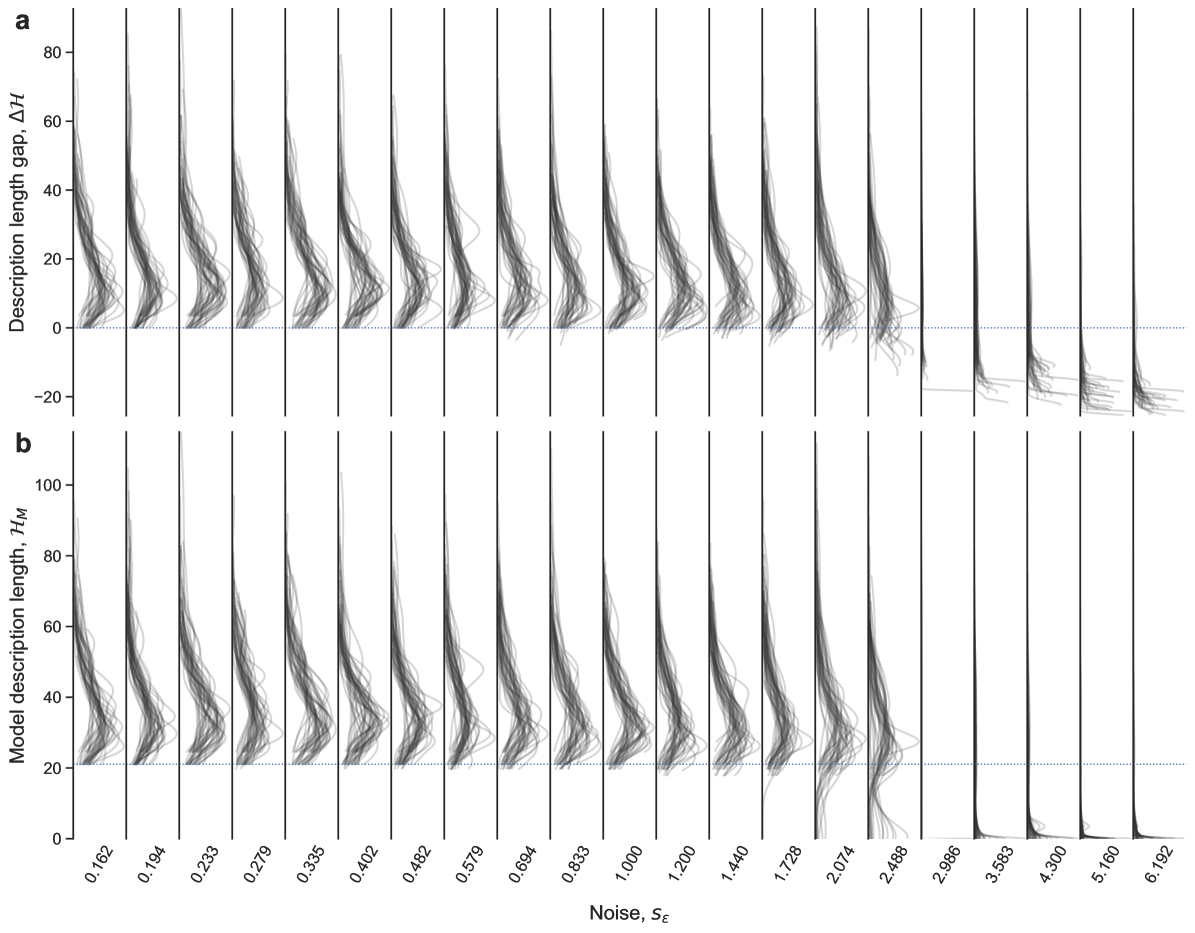
Next, we establish the existence of the learnable and unlearnable regimes, and clarify how the transition between them happens. Again, we generate synthetic data $D$ using a known model $m^{*}$ as in the previous section, and sample models from the posterior $p(m|D)$. To investigate whether a model is learnable we consider the ensemble of sampled models (Fig. 2); if no model in the ensemble is more plausible than the true generating model (that is, if the true model is also the MDL model), then we conclude that the model is learnable. Otherwise, the model is unlearnable because lacking any additional information about the generating model, it is impossible to identify it, as other models provide more parsimonious descriptions of the data $D$.

To this end, we first consider the gap $\Delta\mathcal{H}(m)=\mathcal{H}(m)-\mathcal{H}(m^{*})$ between the description length of each sampled model $m$ and that of the true generating model $m^{*}$ (Fig. 2a). For low observation error $s_{\epsilon}$, all sampled models have positive gaps, that is, description lengths that are longer than or equal to the true model. This indicates that the most plausible model is the true model; therefore, the true model is learnable. By contrast, when observation error grows ($s_{\epsilon}\gtrsim 0.6$ in Fig. 2a), some of the models sampled for some training datasets $D$ start to have negative gaps, which means that, for those datasets, these models become more plausible than the true model. When this happens, the true model becomes unlearnable. For even larger values of $s_{\epsilon}$ ($s_{\epsilon}>2$), the true model is unlearnable for virtually all training sets $D$.

To better characterize the sampled models, we next compute description length of the model; that is, the term ${\mathcal{H}_{M}}(m)=-\ln p(m)$ in the description length, which measures the complexity of the model regardless of the data (Fig. 2b). For convenience we set an arbitrary origin for ${\mathcal{H}_{M}}(m)$ so that ${\mathcal{H}_{M}}(m^{c})=0$ for the models $m^{c}=\arg\max_{m}p(m)=\arg\min_{m}{\mathcal{H}_{M}}(m)$ that are most plausible a priori, which we refer to as trivial models; all other models have ${\mathcal{H}_{M}}(m)>0$. We observe that, for low observation error, most of the sampled models are more complex than the true model. Above a certain level of noise ($s_{\epsilon}\gtrsim 3$), however, most sampled models are trivial or very simple models with ${\mathcal{H}_{M}}(m)\approx 0$. These trivial models appear suddenly—at $s_{\epsilon}<2$ almost no trivial models are sampled at all.

Altogether, our analysis shows that for low enough observation error the true model is always recovered. Conversely, in the opposite limit only trivial models (those that are most plausible in the prior distribution) are considered reasonable descriptions of the data. Importantly, our analysis shows that trivial models appear suddenly as one increases the level of noise, which suggests that the transition to the unlearnable regime may be akin to a phase transition driven by changes in the model plausibility (or description length) landscape, similarly to what happens in other problems in inference, constraint satisfaction, and optimization Mézard and Montanari (2009); Zdeborová and Krzakala (2016).

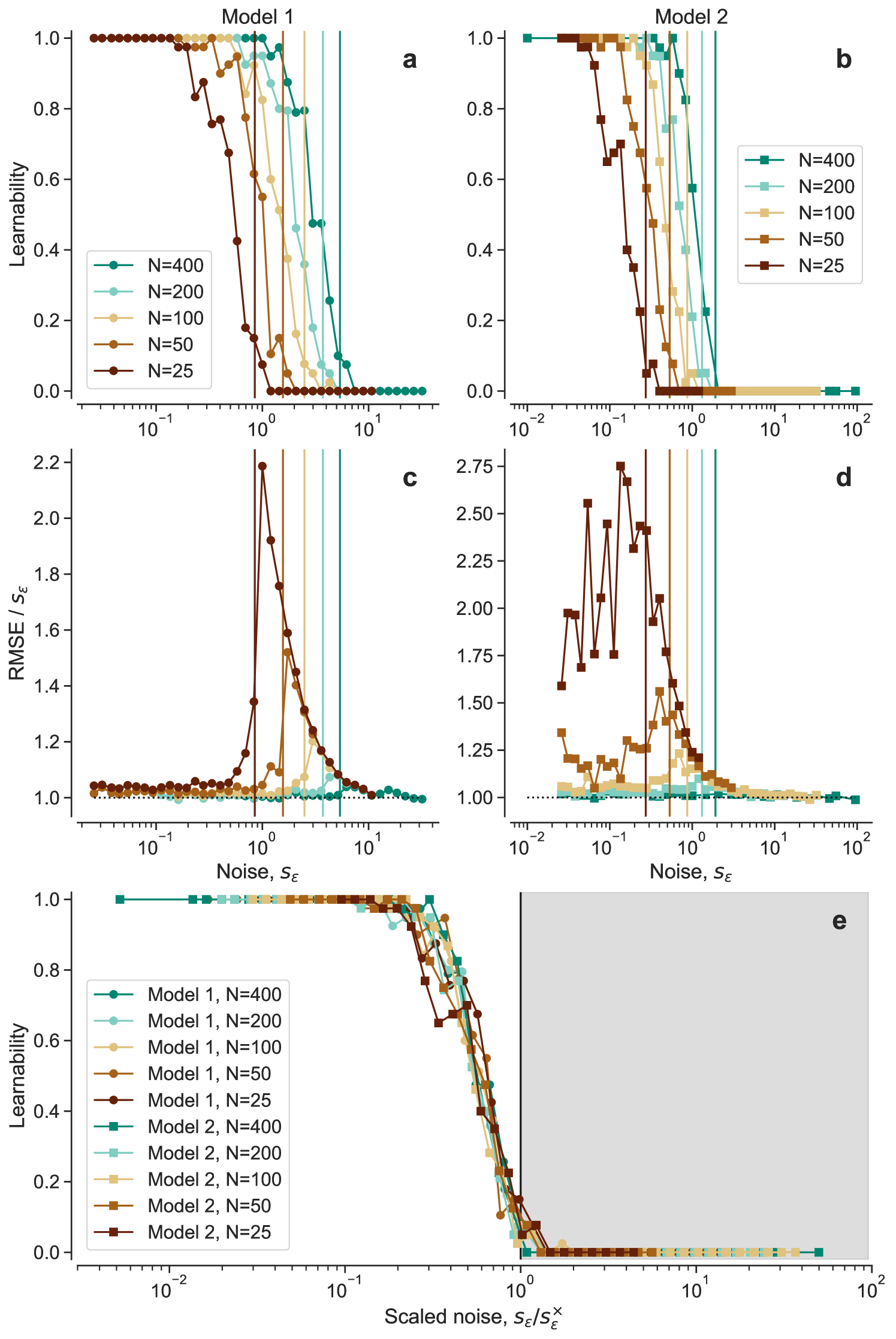
To further probe whether that is the case, we analyze the transition in more detail. Our previous analysis shows that learnability is a property of the training dataset $D$, so that, for the same level of observation noise, some instances of $D$ enable learning of the true model whereas others do not. Thus, by analogy with satisfiability transitions Mézard and Montanari (2009), we define the learnability ${\rho}(s_{\epsilon})$ as the fraction of training datasets $D$ at a given noise $s_{\epsilon}$ for which the true generating model is learnable. In Fig. 3, we show the behavior of the learnability ${\rho}(s_{\epsilon})$ for different sizes $N$, for the two models in Fig. 1 (see Supplementary Fig. S1 for another model). Consistent with the qualitative description above, we observe that the learnability transition occurs abruptly at a certain value of the observation noise; the transition shifts towards higher values of $s_{\epsilon}$ with increasing size of $D$.

Remarkably, the difficult region identified in the previous section, in which prediction error deviates from the theoretical irreducible error $s_{\epsilon}$, coincides with the transition region. Therefore, our results paint a picture with three qualitatively distinct regimes: a learnable regime in which the true model can always be learned and predictions about unobserved data are optimal; an unlearnable regime in which the true model can never be learned but predictions are still optimal because error is driven by observation noise and not by the model itself; and a transition regime in which the true model is learnable only sometimes, and in which predictions are, on average, suboptimal. This, again, is reminiscent of the hard phase in satisfiability transitions and of other statistical learning problems Mézard and Montanari (2009); Ricci-Tersenghi et al. (2019); Maillard et al. (2020).

Finally, we obtain an upper bound to the learnability transition point by assuming that all the phenomenology of the transtion can be explained by the competition between just two minima of the description length landscape $\mathcal{H}(m)$: the minimum corresponding to the true model $m^{*}$; and the minimum corresponding to the trivial model $m^{c}$ that is most plausible a priori

As noted earlier, $m^{c}$ is such that ${\mathcal{H}_{M}}(m^{c})=0$ by our choice of origin ³³3Note that, although the origin of descriptions lengths is not arbitrary, this choice is innocuous as long as we are only concerned with comparisons between models., and for our choice of priors it corresponds to trivial models without any operation, such as $m(\mathbf{x})={\rm const.}$ or $m(\mathbf{x})=x_{1}$. Below, we focus on one of these models $m(\mathbf{x})={\rm const.}$, but our arguments (not the precise calculations) remain valid for any other choice of prior and the corresponding $m^{c}$.

As we have also noted above, the true model is learnable when the description length gap $\Delta\mathcal{H}(m)=\mathcal{H}(m)-\mathcal{H}(m^{*})$ is strictly positive for all models $m\neq m^{*}$. Conversely, the true model $m^{*}$ becomes unlearnable when $\Delta\mathcal{H}(m)=0$ for some model $m\neq m^{*}$. As per our assumption that the only relevant minima are those corresponding to $m^{*}$ and $m^{c}$, we therefore postulate that the transition occurs when the description length gap of the trivial model becomes, on average (over datasets), $\Delta\mathcal{H}(m^{c})=0$. In fact, when $\mathcal{H}(m^{c})\leq\mathcal{H}(m^{*})$ the true model is certainly unlearnable; but other models $m$ could fullfill the condition $\mathcal{H}(m)\leq\mathcal{H}(m^{*})$ earlier, thus making the true model unlearnable at lower observation noises. Therefore, the condition $\Delta\mathcal{H}(m^{c})=0$ yields an upper bound to the value of the noise at which the learnability transition happens. We come back to this issue later, but for now we ignore all potential intermediate models.

Within the BIC approximation, the description length of each of these two models is (Methods)

where $k^{*}$ is the number of parameters of the true model, $\delta_{i}=m^{c}_{i}-m^{*}_{i}$ is the reducible error of the trivial model, and the averages $\langle\cdots\rangle_{D}$ are over the observations $i$ in $D$. Then, over many realizations of $D$, the transition occurs on average at

where $\langle\delta^{2}\rangle$ is now the variance of $m^{*}$ over the observation interval rather than in any particular dataset.

For large $N\gtrsim 100$ and model description lengths of the true model such that $\Delta_{M}^{*}\equiv\mathcal{H}_{M}(m^{*})-\mathcal{H}_{M}(m^{c})\sim O(1)$, the transition noise is well approximated by (Methods)

Therefore, since $s_{\epsilon}^{\times}$ diverges for $N\rightarrow\infty$, the true model is learnable for any finite observation noise, provided that $N$ is large enough (which is just another way of seeing that probabilistic model selection with the BIC approximation is consistent Schwarz (1978)).

In Fig. 3, we show that the upper bound in Eq. (8) is close to the exact transition point from the learnable to the unlearnable phase, as well as to the peak of the prediction error relative to the irreducible error. Moreover, once represented as a function of the scaled noise $s_{\epsilon}/s_{\epsilon}^{\times}$, the learnability curves of both models collapse into a single curve (Fig. 3e), suggesting that the behavior at the transition may be universal. Additionally, the transition between $m^{*}$ and $m^{c}$ becomes more abrupt with increasing $N$, as the fluctuations in $\langle\delta\rangle_{D}$ become smaller. If this upper bound became tighter with increasing $N$, this would be indicative of a true, discontinuous phase transition between the learnable and the unlearnable phases.

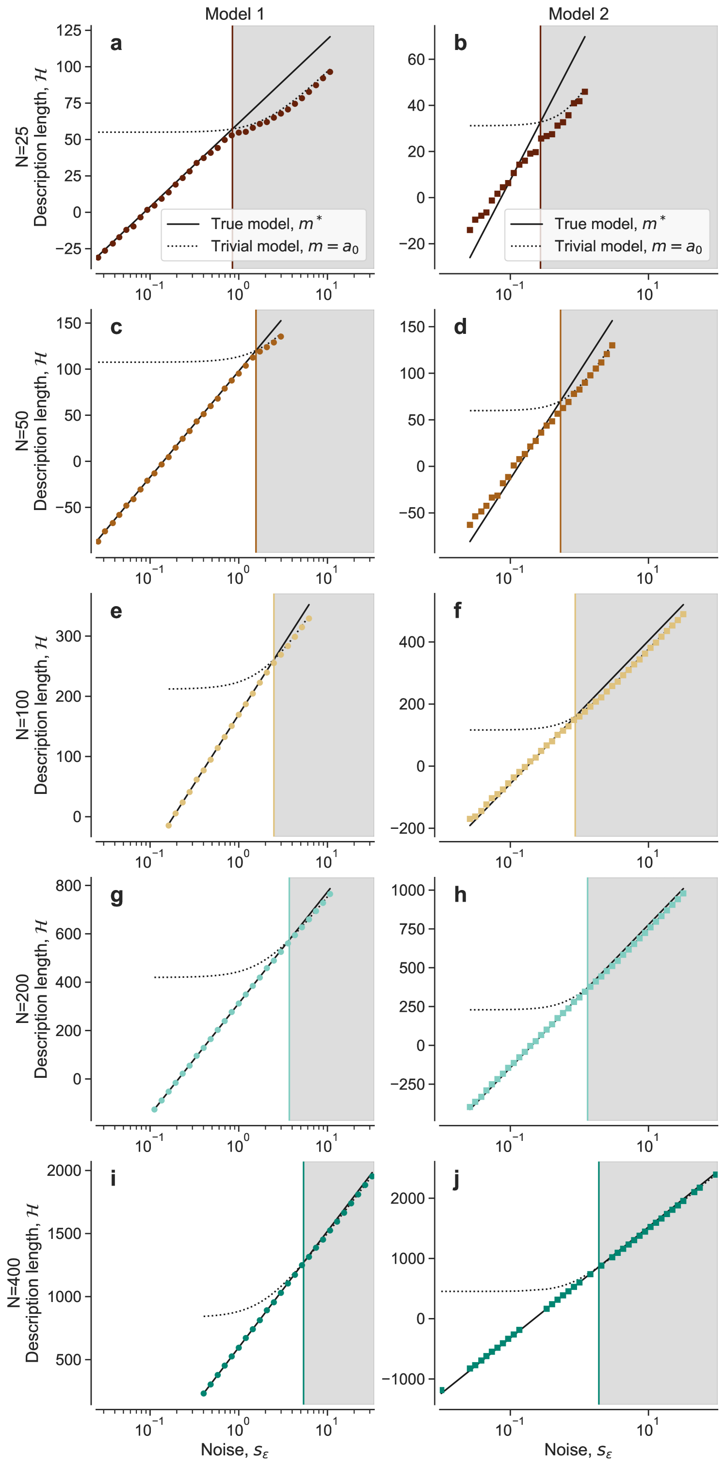
To further understand the transition and further test the validity of the assumption leading to the upper bound $s_{\epsilon}^{\times}$, we plot the average description length (over datasets $D$) of the MDL model at each level of observation noise $s_{\epsilon}$ (Fig. 4). We observe that the description length of the MDL model coincides with the description length $\mathcal{H}(m^{*})$ of the true model below the transition observation noise, and with the description length $\mathcal{H}(m^{c})$ of the trivial model above the transition observation noise. Around $s_{\epsilon}^{\times}$, and especially for smaller $N$, the observed MDL is lower than both $\mathcal{H}(m^{*})$ and $\mathcal{H}(m^{c})$, suggesting that, in the transition region, a multiplicity of models (or Rashomon set Rudin (2019)) other than $m^{*}$ and $m^{c}$ become relevant.

The probabilistic formulation of the model selection problem outline in Eqs. 1–4 requires the choice of a prior distribution $p(m)$ over models—although the general, qualitative results described in the body of the text do not depend on a particular choice of prior. Indeed, no matter how priors are chosen, some model $m^{c}=\arg\max_{m}p(m)$ (or, at most, a finite subset of models, since uniform priors cannot be used Guimerà et al. (2020)) different from the true generating model $m^{*}$ will be most plausible a priori, so the key arguments in the main text hold.

However, the specific, quantitative results must be obtained for one specification of $p(m)$. Here, as in the previous literature Guimerà et al. (2020); Reichardt et al. (2020), we choose $p(m)$ to be the maximum entropy distribution that is compatible with an empirical corpus of mathematical equations Guimerà et al. (2020). In particular, we impose that the mean number $\langle n_{o}\rangle$ of occurrences of each operation $o\in\{+,*,\exp,\dots\}$ per equation is the same as in the empirical corpus; and that the fluctuations of these numbers $\langle n_{o}^{2}\rangle$ are also as in the corpus. Therefore, the prior is

where $\mathcal{O}=\{+,*,\exp,\dots\}$, and the hyperparameters $\alpha_{o}\geq 0$ and $\beta_{o}\geq 0$ are chosen so as to reproduce the statistical features of the empirical corpus Guimerà et al. (2020). For this particular choice of prior, the models $m^{c}=\arg\max_{m}p(m)$ are those that contain no operations at all, for example $m^{c}={\rm const.}$; hence the use of the term trivial to denote these models in the text.

For a given dataset $D$, each model $m$ has a description length $\mathcal{H}(m)$ given by Eq. (4). The Bayesian machine scientist Guimerà et al. (2020) generates a Markov chain of models $\{m_{0},m_{1},\dots,m_{T}\}$ using the Metropolis algorithm as described next.

Each model is represented as an expression tree, and each new model $m_{t+1}$ in the Markov chain is proposed from the previous one $m_{t}$ by changing the corresponding expression tree: changing an operation or a variable in the expression tree (for example, proposing a new model $m_{t+1}=\theta_{0}+x_{1}$ from $m_{t}=\theta_{0}*x_{1}$); adding a new term to the tree (for example, $m_{t+1}=\theta_{0}*x_{1}+x_{2}$ from $m_{t}=\theta_{0}*x_{1}$); or replacing one block of the tree (for example, $m_{t+1}=\theta_{0}*\exp(x_{2})$ from $m_{t}=\theta_{0}*x_{1}$) (see Guimerà et al. (2020) for details). Once a new model $m_{t+1}$ is proposed from $m_{t}$, the new model is accepted using the Metropolis rule.

Note that the only input to the Bayesian machine is the observed data $D$. In particular, the observational noise $s\epsilon$ is unknown and must be estimated, via maximum likelihood, to calculate the Bayesian information criterion $B(m)$ of each model $m$.

For the analysis of predictions on unobserved data, we use as benchmarks the following artificial neural network architectures and training procedures. The networks consist of: an input layer with two inputs corresponding to $x_{1}$ and $x_{2}$; (ii) four hidden fully connected feed-forward layers, with 10 units each and ReLU activation functions; and (iii) a linear output layer with a single output $y$.

Each network was trained with a dataset $D$ containing $N$ points, just as in the probabilistic model selection experiments. Training errors and validation errors (computed on an independent set) were calculated, and the training process stopped when the validation error increased, on average, for 100 epochs; this typically entailed training for 1,000-2,000 epochs. This procedure was repeated three times, and the model with the overall lowest validation error was kept for making predictions on a final test set $D^{\prime}$. The predictions on $D^{\prime}$ are those reported in Fig. 1.

The description length of a model is given by Eq. (4), and the BIC is

where $\left.{\cal L}(m)\right|_{\hat{\theta}}=p(D|m,\hat{\theta})$ is the likelihood of the model calculated at the maximum likelihood estimator of the parameters, $\hat{\theta}=\arg\max_{\theta}p(D|m,\theta)$, and $k$ is the number of parameters in $m$. In a model-selection setting, one would typically assume that the deviations of the observed data are normally distributed independent variables, so that

where $m_{i}\equiv m(\mathbf{x}_{i})$, and ${s_{y}}$ is the observed error, which in general differs from $s_{\epsilon}$ when $m\neq m^{*}$. We can obtain the maximum likelihood estimator for ${s_{y}}^{2}$, which gives ${s_{y}}^{2}=\frac{1}{N}\sum_{i}(y_{i}-m^{*}_{i})^{2}$, and replacing into Eqs. (4)-(12) gives

For $m=m^{*}$ we have that ${s_{y}}^{2}=\frac{1}{N}\sum_{i}(y_{i}-m^{*}_{i})^{2}=\langle\epsilon^{2}\rangle_{D}$. For any other model $m$, we define for each point the deviation from the original model $\delta_{i}:=m_{i}-m^{*}_{i}$ so that ${s_{y}}^{2}=\frac{1}{N}\sum_{i}(\epsilon_{i}-\delta_{i})^{2}=\langle\epsilon^{2}\rangle_{D}+\langle\delta^{2}\rangle_{D}-2\langle\delta\epsilon\rangle_{D}$. Plugging these expressions into Eq. (13), we obtain the expressions in Eqs. (6) and  (7).

Defining $x=1/N$ in Eq. (8) and using the Puiseux series expansion

around $x=0$, we obtain Eq. (9).

References

- Džeroski and Todorovski (2007) S. Džeroski and L. Todorovski, eds., Computational Discovery of Scientific Knowledge, Lecture Notes in Artificial Intelligence (Springer, 2007).
- Schmidt and Lipson (2009) M. Schmidt and H. Lipson, Science 324, 81 (2009).
- Evans and Rzhetsky (2010) J. Evans and A. Rzhetsky, Science 329, 399 (2010).
- Brunton et al. (2016) S. L. Brunton, J. L. Proctor, and J. N. Kutz, Proc. Natl. Acad. Sci. U.S.A. 113, 3932 (2016).
- Guimerà et al. (2020) R. Guimerà, I. Reichardt, A. Aguilar-Mogas, F. A. Massucci, M. Miranda, J. Pallarès, and M. Sales-Pardo, Sci. Adv. 6, eaav6971 (2020).
- Udrescu and Tegmark (2020) S.-M. Udrescu and M. Tegmark, Sci. Adv. 6, eaay2631 (2020).
- Note (1) Here and throughout this article, we refer to closed-form models as those that are expressed in terms of a relatively small number of basic functions, such as addition, multiplication, trigonometric functions, etc.
- Gentile et al. (2021) A. A. Gentile, B. Flynn, S. Knauer, N. Wiebe, S. Paesani, C. E. Granade, J. G. Rarity, R. Santagati, and A. Laing, Nat. Phys. 17, 837 (2021).
- Reichardt et al. (2020) I. Reichardt, J. Pallarès, M. Sales-Pardo, and R. Guimerà, Phys. Rev. Lett. 124, 084503 (2020).
- Cranmer et al. (2020) M. Cranmer, A. Sanchez Gonzalez, P. Battaglia, R. Xu, K. Cranmer, D. Spergel, and S. Ho, in Advances in Neural Information Processing Systems, Vol. 33, edited by H. Larochelle, M. Ranzato, R. Hadsell, M. F. Balcan, and H. Lin (Curran Associates, Inc., 2020) pp. 17429–17442.
- Note (2) The assumption of Gaussian noise is standard in regression and symbolic regression problems, and it allows us to write the likelihood as in Eq. (12\@@italiccorr). In principle, one could assume other noise structures (for example, multiplicative noise) or even more general likelihoods, but these would be hard to justify in the context of regression and symbolic regression/model discovery. In any case, we do not expect that the qualitative behavior described in the manuscript should change in any way.
- Zdeborová and Krzakala (2016) L. Zdeborová and F. Krzakala, Adv. Phys. 65, 453 (2016).
- Schwarz (1978) G. Schwarz, Ann. Stat. 6, 461 (1978).
- Grünwald (2007) P. D. Grünwald, The Minimum Description Length Principle (The MIT Press, Cambridge, Massachusetts, 2007).
- Cox (1946) R. T. Cox, Am. J. Phys. 14, 1 (1946).
- Jaynes (2003) E. T. Jaynes, Probability Theory: The Logic of Science (Cambridge University Press, 2003).
- Mézard and Montanari (2009) M. Mézard and A. Montanari, Information, Physics, and Computation (Oxford University Press, 2009).
- Ricci-Tersenghi et al. (2019) F. Ricci-Tersenghi, G. Semerjian, and L. Zdeborová, Phys. Rev. E 99, 042109 (2019).
- Maillard et al. (2020) A. Maillard, B. Loureiro, F. Krzakala, and L. Zdeborová, in Advances in Neural Information Processing Systems, Vol. 33, edited by H. Larochelle, M. Ranzato, R. Hadsell, M. Balcan, and H. Lin (Curran Associates, Inc., 2020) pp. 11071–11082.
- Note (3) Note that, although the origin of descriptions lengths is not arbitrary, this choice is innocuous as long as we are only concerned with comparisons between models.
- Rudin (2019) C. Rudin, Nat. Mach. Intell. 1, 206 (2019).
- Carleo et al. (2019) G. Carleo, I. Cirac, K. Cranmer, L. Daudet, M. Schuld, N. Tishby, L. Vogt-Maranto, and L. Zdeborová, Rev. Mod. Phys. 91, 45002 (2019).
- Engel and den Broeck (2004) A. Engel and C. V. den Broeck, Statistical Mechanics of Learning (Cambridge University Press, Cambridge, UK, 2004).
- Aubin et al. (2020) B. Aubin, F. Krzakala, Y. Lu, and L. Zdeborová, in Advances in Neural Information Processing Systems, Vol. 33, edited by H. Larochelle, M. Ranzato, R. Hadsell, M. Balcan, and H. L. n (Curran Associates, Inc., 2020) pp. 12199–12210.
- Mignacco et al. (2022) F. Mignacco, F. Krzakala, Y. M. Lu, P. Urbani, and L. Zdeborová, in Proceedings of the 37th International Conference on Machine Learning, ICML’20 (JMLR.org, 2022).
- Guimerà and Sales-Pardo (2009) R. Guimerà and M. Sales-Pardo, Proc. Natl. Acad. Sci. U. S. A. 106, 22073 (2009).
- Decelle et al. (2011) A. Decelle, F. Krzakala, C. Moore, and L. Zdeborová, Phys. Rev. Lett. 107, 065701 (2011).
- Krzakala et al. (2016) F. Krzakala, F. Ricci-Tersenghi, L. Zdeborová, R. Zecchina, E. W. Tramel, and L. F. Cugliandolo, eds., Statistical Physics, Optimization, Inference, and Message-Passing Algorithms, 1st ed. (Oxford, UK, 2016).
- Vallès-Català et al. (2018) T. Vallès-Català, T. P. Peixoto, M. Sales-Pardo, and R. Guimerà, Phys. Rev. E 97, 062316 (2018).
- Peixoto (2020) T. P. Peixoto, “Advances in network clustering and blockmodeling,” (John Wiley & Sons Ltd, 2020) Chap. Bayesian stochastic blockmodeling.
- Ando (2010) T. Ando, Bayesian model selection and statistical modeling (CRC Press, 2010).
- Mondelli and Montanari (2019) M. Mondelli and A. Montanari, Foundations of Computational Mathematics 19, 703 (2019).
- Barbier et al. (2019) J. Barbier, F. Krzakala, N. Macris, L. Miolane, and L. Zdeborová, Proc. Natl. Acad. Sci. U.S.A. 116, 5451 (2019).
Acknowledgements.
This research was funded by project PID2019-106811GB-C31 from the Spanish MCIN/AEI/10.13039/501100011033 and by the Government of Catalonia (2017SGR-896).Author contributions
MS-P and RG designed the research. OF-F, IR, HDLR, and RG wrote code and run computational experiments. All authors analyzed data. OF-F, IR, MS-P, and RG wrote the manuscript.
Competing interests
The authors declare no competing interests.