funOCLUST: Clustering Functional Data with Outliers
Abstract
Functional data present unique challenges for clustering due to their infinite-dimensional nature and potential sensitivity to outliers. An extension of the OCLUST algorithm to the functional setting is proposed to address these issues. The approach leverages the OCLUST framework, creating a robust method to cluster curves and trim outliers. The methodology is evaluated on both simulated and real-world functional datasets, demonstrating strong performance in clustering and outlier identification.
Keywords: OCLUST, curves, mixture models, outliers.
1 Background
1.1 OCLUST Algorithm
Clustering is a subtype of classification, which aims to group similar sets of observations together without any prior knowledge of the cluster memberships. While non-parametric methods exist, e.g., hierarchical and k-means clustering, model-based clustering employs a parametric approach. In general, the density of a finite mixture model is
| (1) |
where , is the th mixing proportion with , and is the th component density with parameters . Typically, each component corresponds to a cluster (see McNicholas, 2016, for a discussion). While each cluster can be modelled with various component distributions, the Gaussian distribution remains popular due to its simplicity. The parameters and cluster memberships are estimated by maximizing the log-likelihood, often with the expectation-maximization (EM) algorithm (Dempster et al., 1977).
Clark and McNicholas (2024) develop the OCLUST algorithm, which simultaneously clusters data and trims outliers. Data are modelled with mixtures of Gaussian distributions, and outliers are trimmed iteratively one-by-one. A subset log-likelihood is defined to be the log-likelihood of the data with a single data point removed, and there are such subsets. After each outlier removal, the distribution of the subset log-likelihoods is compared to the mixture of shifted and scaled beta distributions derived in the paper. Specifically, let be the complete-data log-likelihood of the entire dataset, let be the complete-data log-likelihood of the th subset, i.e., with observation removed, and let . Then, if belongs to the th cluster, i.e. with indicator variable ,
| (2) |
for , where , is the number of points in cluster , ,
is the sample covariance matrix of cluster , and The trimmed model chosen minimizes the Kullback-Leibler (KL) divergence between the observed differences and the derived distribution.
1.2 Functional Decomposition
In multivariate data analysis, a random sample ( is typically a collection of vectors in . In functional data, a random sample of functions ( exists in infinite-dimensional space. In practice, however, these functions are evaluated at a series of discrete values , resulting in observations of the form , where is a vector of points in the domain and is the vector of observed values at the points . To return to infinite-dimensional space, we can reconstruct the functional form. A popular choice is a basis expansion, which is well explained by Ramsay and Silverman (2005).
In a basis expansion, the function is approximated by a linear combination of basis functions so that , where is the value at for the th basis function. Basis functions must be independent from each other and must be able to approximate any function with reasonable accuracy. Some choices for basis functions are Fourier series, wavelet functions, power series, exponential, polynomial and power bases, as well as B-spline basis functions. Functional principal components analysis (FPCA) is a special type of basis expansion, where is approximated by a linear combination of mutually orthogonal and normalized weight functions that explain decreasing amounts of variation in the sample (.
1.3 Clustering Functional Data
Jacques and Preda (2014) organize functional data clustering into three paradigms — two-stage methods, nonparametric methods and model-based methods. In model-based approaches, the filtering and clustering steps are completed simultaneously. James and Sugar (2003) introduce a Gaussian mixture model for functional clustering by assuming that the coefficients in the basis expansion are normally-distributed. These coefficients are not fixed– they are estimated within the EM algorithm. Similarly, Jacques and Preda (2013) generate a Gaussian mixture model with FPCA scores. Bouveyron and Jacques (2011) combine the model of James and Sugar (2003) with the assumption that each cluster lies in a lower-dimensional subspace, thus reducing the dimension when there are large numbers of basis functions. The resultant algorithm is called funHDDC.
A similar, more general, approach is to treat the functions as finite mixtures of regressions:
| (3) |
where is a regression matrix, which may be constructed from polynomials, splines, or B-splines, etc. Extensions to this method are regularized regression mixtures and the regression mixtures with mixed-effects (Chamroukhi and Nguyen, 2019).
Abraham et al. (2003) propose a two-stage approach, first filtering the data with a B-spline basis and then clustering the resulting coefficients with the -means algorithm. In this case, because the filtering is completed first, the coefficients are fixed. Similarly, Peng and Müller (2008) first use FPCA to decompose the functions. The FPCA scores are then scaled and clustered using -means clustering. Nguyen et al. (2018) propose a two-part algorithm, first fitting the B-spline basis coefficients to the functions, and then applying a Gaussian mixture model to those coefficients. They suppose that is a random variable described by a Gaussian mixture model. Then the distribution of the fitted coefficients, can be described as a mixture model with density
| (4) |
1.4 Outliers in Functional Data Clustering
Hubert et al. (2015) separate functional outliers into two types: isolated outliers and persistent outliers. While isolated outliers are atypical in a narrow region, e.g., a spike, persistent outliers affect a larger portion of the domain, e.g., shift, amplitude, or shape. In functional data clustering, algorithms that handle outliers also belong to the three paradigms in Section 1.3. Using a two-stage approach, Garcia-Escudero and Gordaliza (2005) propose a method to cluster functional data with outliers by first decomposing the functions using a B-spline basis, and then clustering the resulting coefficients with trimmed -means clustering.
In the model-based realm, funHDDC has been extended to be more robust to outliers. Amovin-Assagba et al. (2022) develop C-funHDDC, which combines a contaminated mixture model with funHDDC by assuming that the functions reside in a lower-dimensional cluster-specific subspace. Similarly, Anton and Smith (2023), use a t-distribution with the funHDDC foundation to generate a more robust model in the presence of outliers, called T-funHDDC.
In a non-parametric approach, a functional isolation forest (FIF; Staerman et al., 2019) is a collection of isolation trees which randomly split the functional space into partitions, iteratively, until each function is isolated. Functions isolated in fewer iterations tend to be more outlying. An outlier score is calculated using a forest of these isolation trees. Finally, Hubert et al. (2015) determine functional outlyingness by first calculating outlyingness at each time point and then taking the weighted average to create an outlier score for each curve.
2 Methodology
2.1 Overview
The OCLUST algorithm hinges on the the fact that log-likelihoods of the data subsets have an approximate shifted and scaled beta distribution. Extending the OCLUST algorithm to functional data will require something similar: a model with an associated log-likelihood function that can be evaluated on data subsets, and for which the distribution of these subset log-likelihoods can be derived.
While functions exist in infinite-dimensional space, they are observed at a series of discrete points . If each curve is sampled at the same points, then the data for each curve can be considered as a vector. If these vectors arise from a finite Gaussian mixture, then there will be an associated log-likelihood for the data and associated parameters , for each component. An obvious choice would be to apply the OCLUST algorithm to the discretized values when modelling a finite Gaussian mixture model of functional data with outliers. However, these vectors will be the same dimension as the number of points at which each function is sampled. To retain enough information about the curve, the vectors of observations are likely to be very high-dimensional.
Instead, consider applying a filtering approach to the raw data, specifically their decomposition with cubic B-splines,
| (5) |
where is the cubic B-spline basis with interior knots evaluated at point , is the vector of coefficients for the basis expansion of function , and is the error term. This retains the infinite-dimensional properties of the functions, and each function has a unique -dimensional representation given by the vector . In effect, each is transformed to a vector in , the dimension of which is governed only by the choice in number of interior knots. Transforming maintains the principle of working with functions while creating a vector representation in a much more manageable dimension. If we assume that the vectors come from a multivariate normal distribution, then the extension of the OCLUST algorithm to functional data becomes straightforward.
2.2 Subsets and the Distribution of Log-Likelihoods
Consider a sample of i.i.d. functions (). Suppose that each can be decomposed into a linear combination of cubic B-splines, i.e., , where . To capture heterogeneity across functional observations and enable clustering of similar functional patterns, Nguyen et al. (2018) propose that each arise from a finite Gaussian mixture model with density
| (6) |
In addition, they show that the fitted coefficients (), corresponding to functions () follow their own Gaussian mixture model with density
| (7) |
where is the matrix of basis functions evaluated at points , the fitted functions are , and the OLS-estimated coefficients are given by , with . Note that all functions are observed at the same time points .
These principles allow us to formulate Lemma 1. Consider the complete set of fitted coefficients generated by decomposing the functions with a cubic B-spline basis with interior knots. Define the th subset
as the set of fitted coefficients for the functions , i.e., the entire sample with the th function removed. Let denote the complete-data log-likelihood
| (8) |
where the complete-data comprise the coefficients and the cluster memberships . Note that when coefficient belongs to cluster , and otherwise.
Lemma 1.
Consider a vector of fitted coefficients generated by decomposing the function using cubic B-spline basis functions with interior knots. If belongs to the th cluster, i.e., , if is the complete-data log-likelihood and , then has an approximate shifted and scaled beta density, i.e.,
| (9) |
for , where , is the number of points in cluster , ,
is the sample covariance matrix of cluster , and is the number of interior knots in the cubic spline basis used to generate .
Proof.
Using the density from (9) we can generate the unconditional density of using a mixture model, i.e.,
| (10) |
where is a shifted and scaled beta density described in (9), and .
Remark 1.
The density in (9) describes under the assumption that each arises from a finite Gaussian mixture model and that there are no outlying coefficients. If (9) fails to describe , then we can conclude that a model assumption has been violated. In this case, we assume that the model is correctly specified apart from the presence of outliers.
2.3 funOCLUST Algorithm
While the distribution in Section 2.2 used the complete-data log-likelihood, we now change to using the traditional log-likelihood, given by
| (11) |
This choice is made because it is outputted by most clustering algorithms. In addition, Clark and McNicholas (2024) show that as the clusters separate. The funOCLUST algorithm removes candidate outliers iteratively until the subset log-likelihoods of the B-spline coefficients conform to the derived distribution. It is thus necessary to define a candidate outlier.
Definition 1 (Candidate Outlier).
We define our candidate outlier as , where
and is the log-likelihood of the subset with the point removed.
The most outlying coefficient is the one whose corresponding log-likelihood is greatest, i.e., the model improved the most in its absence. When treating the coefficients as a multivariate normal dataset, this is consistent with the OCLUST algorithm. However, before proceeding, it is necessary to establish that a function is outlying when its set of coefficients is outlying in terms of multivariate normality.
Lemma 2.
A function is outlying if is outlying, where
| (12) |
is the matrix of cubic B-spline basis functions with interior knots, and is the error term, i.e., .
Proof.
Consider a potential outlier created by linearly transforming the mean coefficient vector, i.e. . The Mahalanobis squared distance of is
| (13) |
Because is positive definite, we have . Thus, applying any transformation to the mean vector will increase the Mahalanobis squared distance, because . Any transformation to the mean vector will also transform the mean function, i.e.
where , and is the mean function.
Because
and (Clark and McNicholas, 2024), candidate outliers have the largest Mahalonobis square distances and thus the largest transformations from the mean function. ∎
Relating this back to the taxonomy of Hubert et al. (2015), isolated outliers have , where is a unit vector aligned with the -axis. Shift outliers have , where is the vector with each entry equal to 1. Amplitude outliers correspond to , with having a dampening effect and having an amplifying effect. Finally, shape outliers correspond to any combination thereof, including where .
The funOCLUST algorithm proceeds in two steps: filtering and then clustering. First, the functions are filtered by decomposing them into linear combinations of cubic B-splines. In the second step, the funOCLUST algorithm clusters the fitted coefficients, and detects outliers. In each iteration of the second step, subsets of the coefficients are clustered and their corresponding log-likelihood recorded. The distribution of these subset log-likelihoods is measured against the theoretical distribution with the KL divergence. The candidate outlier is then removed before the next iteration begins. The model is free of outliers when KL is minimized. Formally, the funOCLUST algorithm is given in Algorithm 1.
3 Simulation Study
In this simulation study, we compare the funOCLUST algorithm to five competitors: funHDDC; T-funHDDC; a robust curve clustering approach called tkmeans (Garcia-Escudero and Gordaliza, 2005); FIF; and functional outlyingness (fOutl; Hubert et al., 2015; Segaert et al., 2024).
Both funHDDC and T-funHDDC are functional clustering methods, with the latter being more robust to outliers. Both tkmeans and funOCLUST cluster and detect outliers simultaneously. FIF and fOutl detect outliers only and do not cluster the functional data. These five methods and funOCLUST are applied to 100 generated datasets with the following properties:
-
•
500 functions are simulated in two clusters with equal proportions;
-
•
functions are sampled at 100 equally-spaced points in the interval ;
-
•
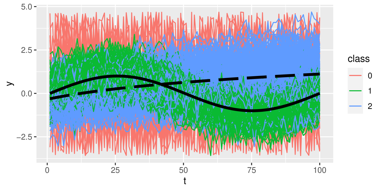
functions in class 1 are simulated from , and functions in class 2 are simulated from , where , , , , and ; and
-
•
15 outliers are generated with each entry uniformly distributed between the minimum and maximum values among all functions and all time points
.
In effect, each function belongs to a ‘family’ of functions corresponding to its class, with random scales, and vertical and horizontal shifts for each function, . In addition, there is an assumed normally-distributed measurement error for each observation. The expected value of each function is for class 1 and for class 2. An example of one of these simulated datasets is shown in Figure 1.
The funOCLUST approach is run, choosing a cubic B-spline basis with 8 equally-spaced interior knots, yielding 12 basis functions. The upper bound is set to 50. For tkmeans, the same basis is chosen and the resulting coefficients are clustered according to a trimmed -means algorithm, using the tclust package (Fritz et al., 2012) for R and preset number of points to trim as 25. The funHDDC and T-funHDDC algorithms are run with the R packages funHDDC (Schmutz and Bouveyron, 2021) and TFunHDDC (Anton and Smith, 2023), respectively, choosing a cubic B-spline basis with 25 basis functions. FIF is run with its Python implementation, available on GitHub (Staerman, 2021), with 100 trees using the cosine dictionary, the classical scalar product, and sample size 64 per tree. The fOutl method is implemented with the fOutl function in the mrfDepth package (Segaert et al., 2024), using adjusted outlyingness with Stahel-Donoho outlyingness (Stahel, 1981; Donoho, 1982) as the distance option.
Each clustering algorithm is evaluated using the adjusted Rand index (ARI; Hubert and Arabie, 1985). The ARI compares two partitions — in this case, real and predicted classes. The ARI equals one under perfect classification and has expected value zero under random class assignment. The funOCLUST and tkmeans approaches are evaluated as three-class solutions, with one of those classes being ‘outlier’. Additionally, the ARI is calculated on the non-outlying points. This serves two purposes: it allows funHDDC and T-funHDDC to be evaluated because they do not identify outliers; and it also evaluates their ability to recover correct classifications of the ‘good’ functions in the presence of noise. The ARI for each clustering algorithm is shown in Table 1 and plotted in Figure 2.
| ARI | ||
|---|---|---|
| Model | mean | sd |
| Full dataset | ||
| funOCLUST | 0.97 | 0.02 |
| tkmeans | 0.50 | 0.06 |
| Dataset without simulated outliers | ||
| T-funHDDC | 0.68 | 0.16 |
| funHDDC | 0.42 | 0.14 |
| funOCLUST | 0.97 | 0.02 |
| tkmeans | 0.47 | 0.06 |
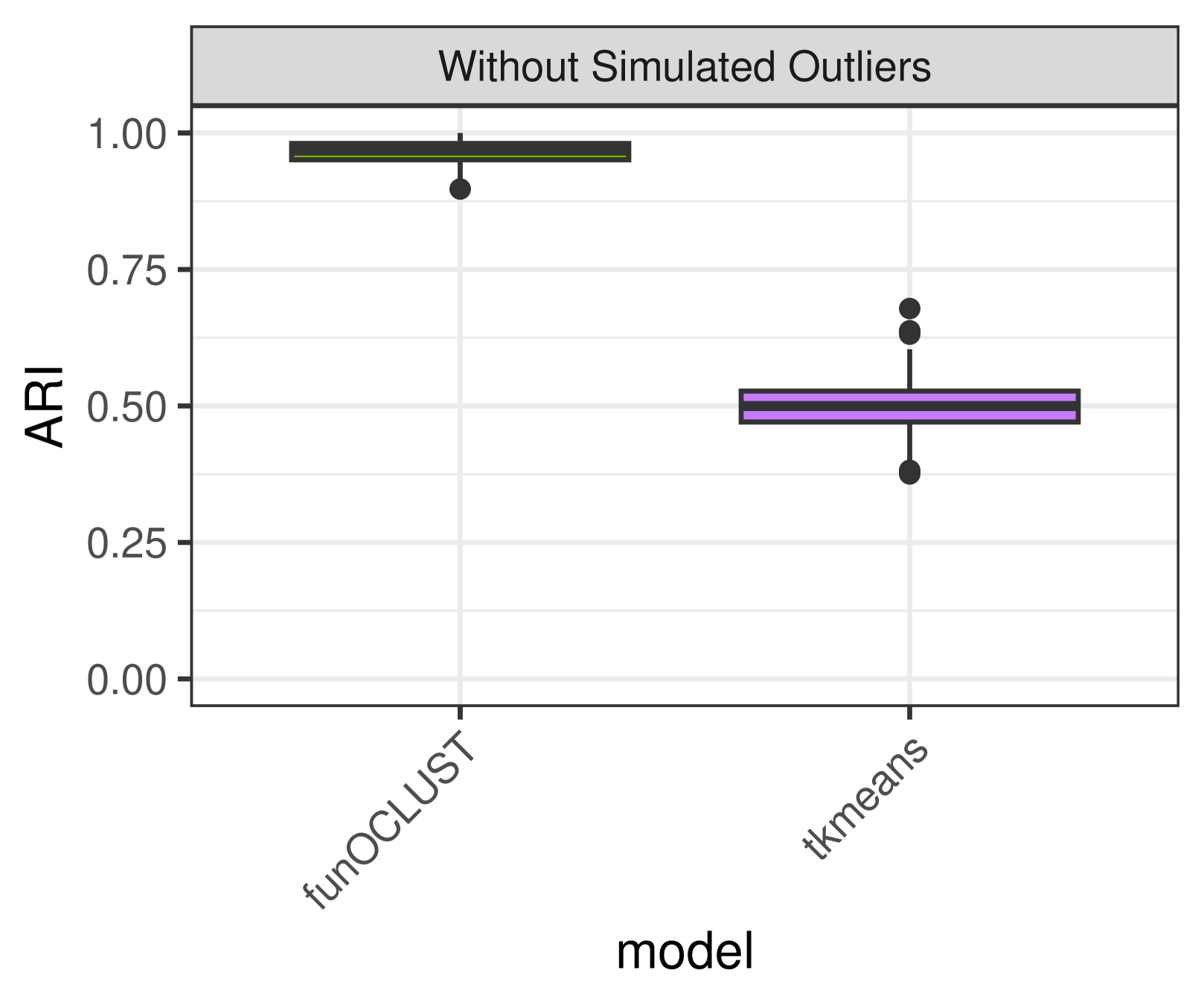
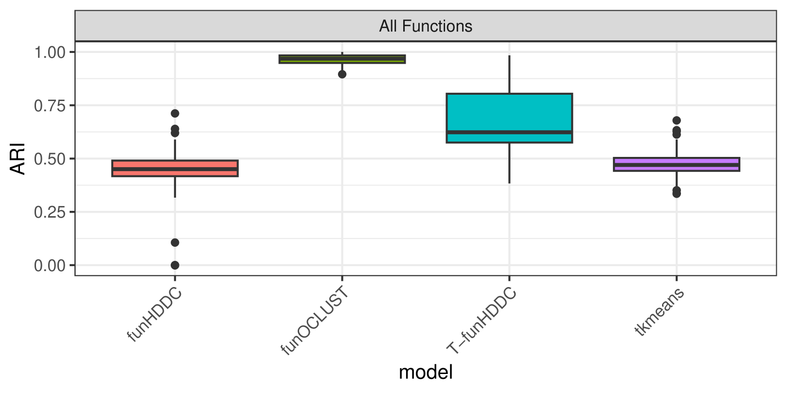
The funOCLUST approach recovers almost perfect classification, with ARI of 0.97 on average. The next best method is T-funHDDC, with average ARI of 0.68. It achieves nearly perfect ARI a few times, but it is not consistent. T-funHDDC outperforms funHDDC, whose average ARI is 0.42, likely due to the increased robustness of the t-distribution. Finally, tkmeans does not perform well, with average ARI of 0.47. While the same coefficients are used in tkmeans and funOCLUST, funOCLUST allows for the coefficients to be correlated. Because is a reflection of , over the x- and y-axes, the coefficients are highly correlated.
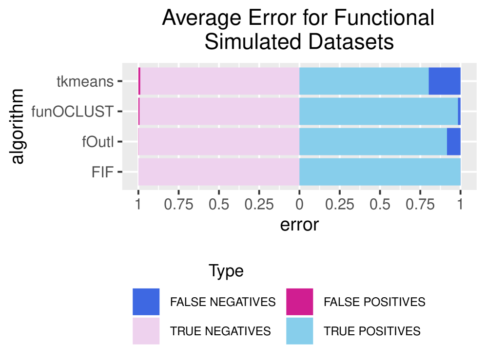
Finally, funOCLUST, tkmeans, FIF, and fOutl are evaluated on their outlier identification accuracy. The FIF algorithm outputs anomaly scores for each function. The scores are similar and smaller for ‘good’ points, but there is a noticeable jump between the last ordered ‘good’ score and the first ‘outlying’ score. We consider scores above this jump to be outliers. Functions are considered outliers using fOutl if their outlyingness exceeds the cutoff from the fom function in the mrfDepth package.
Figure 3 shows false positive rates (dark pink) and false negative rates (dark blue). FIF has excellent outlier identification, with perfect outlier classification on 99 datasets and only one outlier missed on the other. There are no false positives. The fOutl approach has a very low false positive rate of 0.2% but a false negative rate of 8.4%. It is important to note, however, that FIF and fOutl do not cluster the functions, which is why there is no ARI. FunOCLUST has low error, with 0.7% false positive rate and 1.6% false negative rate. On average, it predicts 28.2 outliers with standard deviation 4.5, showing that it tends to slightly overestimate the true number of outliers. While tkmeans has low false positive rate, it has much higher false negative rate. Because the number of functions to trim is set in advance, each ‘good’ function misclassified as an outlier has a corresponding outlying function classified as a ‘good’ one. Because there are far fewer outliers than ‘good’ points, the false negative rate is much higher.
4 Real Data Example
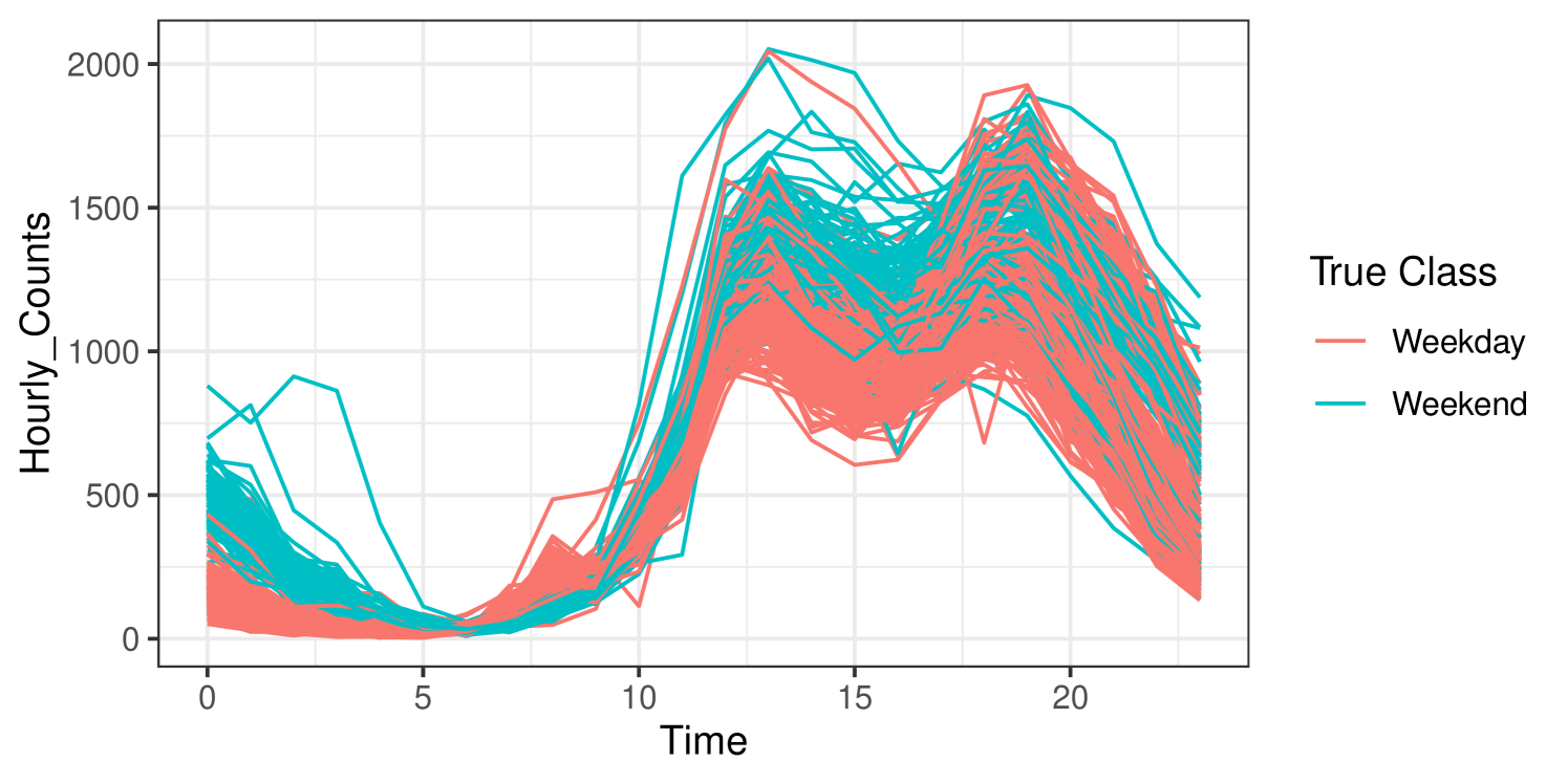
Consider real data on pedestrian traffic in Melbourne, Australia, where sensors installed around the city capture the number of pedestrians passing by each hour. The data are available on kaggle.com (Aadimator, 2022) for all sensors between the years 2009 and 2022. Data captured for the year 2017 from the Chinatown–Swanston St. (North) sensor are plotted in Figure 4, with observations coloured according whether the data correspond to a weekday or weekend. There are 365 observations, each with values collected at 24 time points. Of the 365 days captured, 105 are weekends, and 260 are weekdays. There is one missing value on October 1st between the hours of 2am and 3am.
The same algorithms used in Section 3 are run on these data. The funOCLUST and tkmeans approaches are run with a cubic B-spline basis with 8 equally-spaced interior knots, i.e., 12 basis functions. The upper bound is set to 50. T-funHDDC and funHDDC use 20 cubic B-spline basis functions. The funHDDC, T-funHDDC, and fOutl methods are unable to cluster functions with missing values, so the missing value is imputed as the mean of all functions at that same time of day. FIF is run with the Gaussian wavelet dictionary because the graph of anomaly scores shows the greatest separation. The clustering results are shown in Table 2 as confusion matrices.
| funHDDC | funOCLUST | T-funHDDC | tkmeans | ||||||||||
|---|---|---|---|---|---|---|---|---|---|---|---|---|---|
| Channel | 1 | 2 | 1 | 2 | bad | 1 | 2 | 1 | 2 | bad | |||
| Weekday | 197 | 63 | 244 | 9 | 7 | 200 | 60 | 195 | 61 | 4 | |||
| Weekend | 42 | 63 | 89 | 16 | 43 | 62 | 36 | 50 | 19 | ||||
The funOCLUST algorithm identifies 23 outliers, so tkmeans is run setting the number of functions to trim to 23. The ARI for funHDDC, funOCLUST, T-funHDDC, and tkmeans are 0.164, 0.809, 0.172, and 0.203, respectively. The ARIs for funOCLUST and tkmeans for only the functions they identify as non-outlying are 0.893 and , respectively. The funOCLUST approach has nearly perfect classification among the non-outlying functions, with nine weekdays misclassified as weekends. They are
-
•
January 2, New Year’s Day;
-
•
January 26, Australia Day;
-
•
March 13, Labour Day;
-
•
April 14, Good Friday;
-
•
April 17, Easter Monday;
-
•
April 25, Anzac Day;
-
•
June 12, Queen’s Birthday;
-
•
September 29, Australian Football League Grand Final Parade; and
-
•
November 7, Melbourne Cup Day.
These nine dates correspond to all public holidays in Melbourne in 2017 that fell on weekdays. Because few employees work on public holidays, it is understandable that the pedestrian traffic on those days would mimic a weekend.
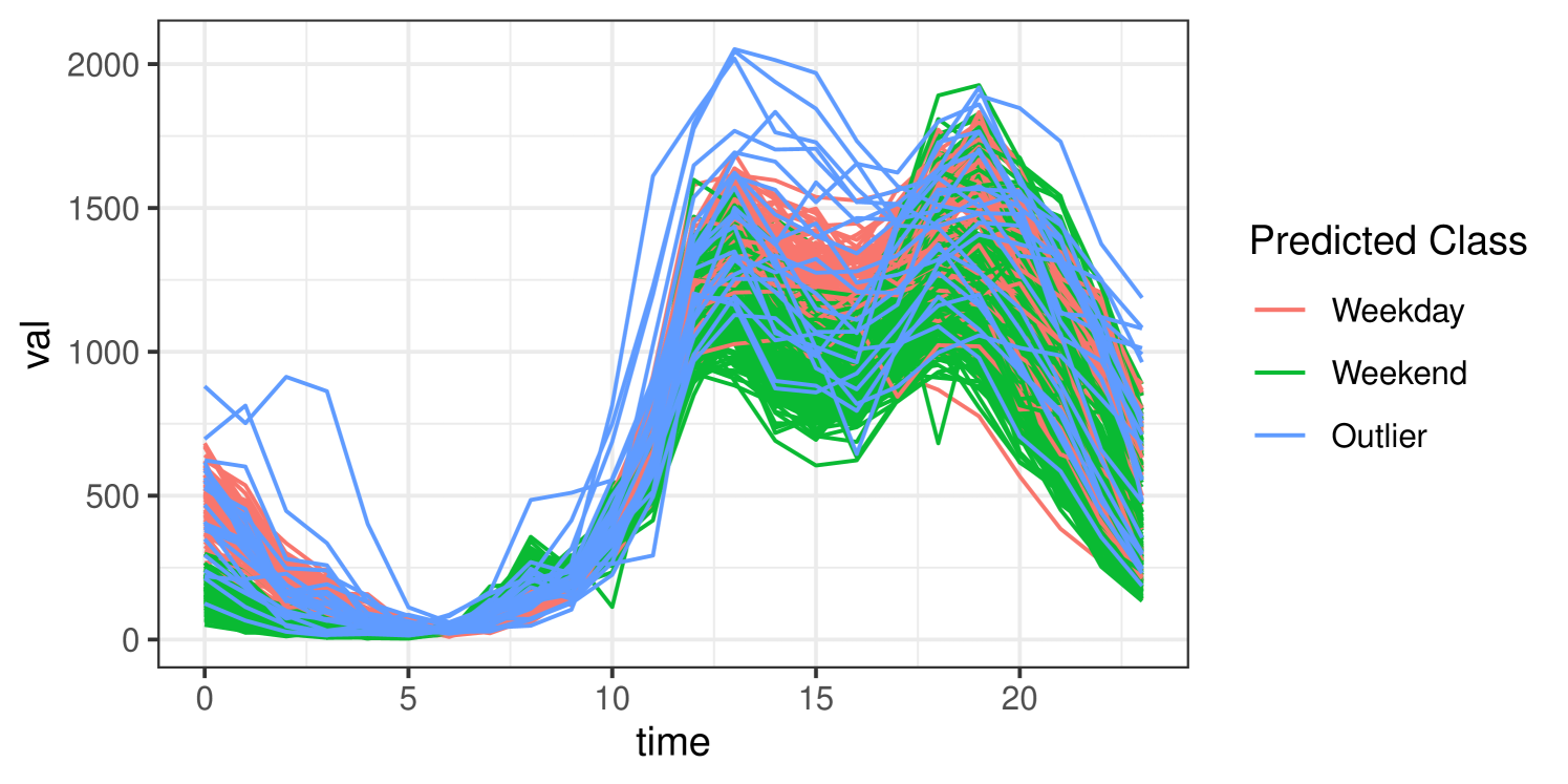
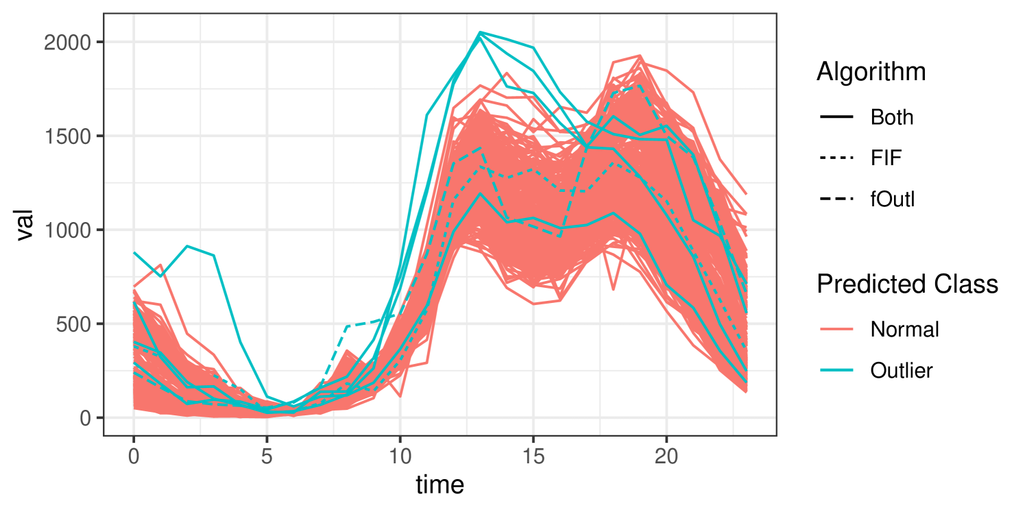
The funOCLUST approach identifies 23 outliers. Included in this list are January 1 (New Year’s Day), December 25 (Christmas Day), December 26 (Boxing Day), January 28–29 (Chinese New Year), and February 18–19 (White Night Melbourne, an all-night arts festival). The funOCLUST solution is plotted in Figure 5, with predicted outliers in blue. Many of the outlying observations have higher-than-average traffic in the afternoon (noon to 5pm) or early morning (midnight to 4am). Additionally, these outliers often exhibit unusual combinations of traffic patterns. For example, traffic volume around noon and 7pm may resemble a typical weekday, while the volume around 4pm is more similar to what is observed on weekends. FIF and fOutl each identify 5 outliers, agreeing on January 29, February 19, August 12, and December 26. FIF identifies October 1 as an additional outlier, while fOutl adds August 11. These six are also identified by funOCLUST as outliers. The curves identified as outlying by FIF and fOutl are plotted in Figure 6. These curves seem to have unusually high values at 1pm or are flatter between 1 and 6pm. August 11th, identified by fOutl, seems to have an unusual combination of high traffic at 6pm with much lower traffic at 4pm.
5 Discussion
The OCLUST algorithm has been extended to functional data. Using an assumption that cubic B-spline coefficients are multivariate normally distributed, the distribution of subset log-likelihoods was derived. This is the basis for the funOCLUST algorithm, which proceeds in two stages. First, functions are transformed using a cubic spline basis, and then the OCLUST algorithm is run, removing candidate outliers one-by-one until the target distribution is reached.
The funOCLUST algorithm showed superior classification performance on both simulated and real datasets. Its outlier identification has error rates second only to FIF, but with the added benefit of clustering simultaneously. When applied to a real dataset on pedestrian traffic in Melbourne, funOCLUST identified certain significant dates as outliers and only misclassified public holidays.
The funOCLUST marks the first extension to OCLUST to functional data. This paves the way for future two-stage extensions, including to multivariate and skewed functional data, and for an OCLUST in the model-based paradigm, where the functional decomposition is estimated within the expectation-maximization algorithm, allowing the model to adapt as outliers are removed.
Acknowledgements
This work was supported by an NSERC Canada Graduate Scholarship, an Ontario Graduate Scholarship, an NSERC Discovery Grant, the Canada Research Chairs program, and a Dorothy Killam Fellowship.
References
- Aadimator (2022) Aadimator (2022). Melbourne pedestrian counting system - monthly. \urlhttps://www.kaggle.com/datasets/aadimator/melbourne-pedestrian-counting-system-monthly?resource=download. Accessed: 2024-07-15.
- Abraham et al. (2003) Abraham, C., P.-A. Cornillon, E. Matzner-Løber, and N. Molinari (2003). Unsupervised curve clustering using b-splines. Scandinavian Journal of Statistics 30(3), 581–595.
- Amovin-Assagba et al. (2022) Amovin-Assagba, M., I. Gannaz, and J. Jacques (2022). Outlier detection in multivariate functional data through a contaminated mixture model. Computational Statistics & Data Analysis 174, 107496.
- Anton and Smith (2023) Anton, C. and I. Smith (2023). Model-based clustering of functional data via mixtures of t distributions. Advances in Data Analysis and Classification.
- Bouveyron and Jacques (2011) Bouveyron, C. and J. Jacques (2011). Model-based clustering of time series in group-specific functional subspaces. Advances in Data Analysis and Classification 5, 281–300.
- Chamroukhi and Nguyen (2019) Chamroukhi, F. and H. D. Nguyen (2019). Model-based clustering and classification of functional data. Wiley Interdisciplinary Reviews: Data Mining and Knowledge Discovery 9(4), e1298.
- Clark and McNicholas (2024) Clark, K. M. and P. D. McNicholas (2024). Finding outliers in Gaussian model-based clustering. Journal of Classification 41(2), 313–337.
- Clark and McNicholas (2025) Clark, K. M. and P. D. McNicholas (2025). oclust: Gaussian Model-Based Clustering with Outliers. R package version 1.0.0.
- Dempster et al. (1977) Dempster, A. P., N. M. Laird, and D. B. Rubin (1977). Maximum likelihood from incomplete data via the EM algorithm. Journal of the Royal Statistical Society: Series B 39(1), 1–38.
- Donoho (1982) Donoho, D. L. (1982). Breakdown properties of multivariate location estimators. Technical report, Harvard University, Boston.
- Fritz et al. (2012) Fritz, H., L. A. García-Escudero, and A. Mayo-Iscar (2012). tclust: An R package for a trimming approach to cluster analysis. Journal of Statistical Software 47(12), 1–26.
- Garcia-Escudero and Gordaliza (2005) Garcia-Escudero, L. A. and A. Gordaliza (2005). A proposal for robust curve clustering. Journal of Classification 22(2), 185–201.
- Hubert and Arabie (1985) Hubert, L. and P. Arabie (1985). Comparing partitions. Journal of Classification 2(1), 193–218.
- Hubert et al. (2015) Hubert, M., P. J. Rousseeuw, and P. Segaert (2015). Multivariate functional outlier detection. Statistical Methods & Applications 24(2), 177–202.
- Jacques and Preda (2013) Jacques, J. and C. Preda (2013). Funclust: A curves clustering method using functional random variables density approximation. Neurocomputing 112, 164–171.
- Jacques and Preda (2014) Jacques, J. and C. Preda (2014). Functional data clustering: a survey. Advances in Data Analysis and Classification 8, 231–255.
- James and Sugar (2003) James, G. M. and C. A. Sugar (2003). Clustering for sparsely sampled functional data. Journal of the American Statistical Association 98(462), 397–408.
- McNicholas (2016) McNicholas, P. D. (2016). Mixture Model-Based Classification. Boca Raton: Chapman & Hall/CRC Press.
- Nguyen et al. (2018) Nguyen, H. D., J. F. Ullmann, G. J. McLachlan, V. Voleti, W. Li, E. M. Hillman, D. C. Reutens, and A. L. Janke (2018). Whole-volume clustering of time series data from zebrafish brain calcium images via mixture modeling. Statistical Analysis and Data Mining: The ASA Data Science Journal 11(1), 5–16.
- Peng and Müller (2008) Peng, J. and H.-G. Müller (2008). Distance-based clustering of sparsely observed stochastic processes, with applications to online auctions. The Annals of Applied Statistics 2(3), 1056 – 1077.
- R Core Team (2025) R Core Team (2025). R: A Language and Environment for Statistical Computing. Vienna, Austria: R Foundation for Statistical Computing.
- Ramsay and Silverman (2005) Ramsay, J. and B. W. Silverman (2005). Functional Data Analysis (2 ed.). New York, NY: Springer.
- Schmutz and Bouveyron (2021) Schmutz, A. and J. J. . C. Bouveyron (2021). funHDDC: Univariate and Multivariate Model-Based Clustering in Group-Specific Functional Subspaces. R package version 2.3.1.
- Segaert et al. (2024) Segaert, P., M. Hubert, P. Rousseeuw, and J. Raymaekers (2024). mrfDepth: Depth Measures in Multivariate, Regression and Functional Settings. R package version 1.0.17.
- Staerman (2021) Staerman, G. (2021). FIF: Functional isolation forest. \urlhttps://github.com/GuillaumeStaermanML/FIF.
- Staerman et al. (2019) Staerman, G., P. Mozharovskyi, S. Clémençon, and F. d’Alché Buc (2019). Functional isolation forest. In Asian Conference on Machine Learning, pp. 332–347. PMLR.
- Stahel (1981) Stahel, W. A. (1981). Robuste schätzungen: infinitesimale optimalität und schätzungen von kovarianzmatrizen. Ph. D. thesis, ETH Zurich.