GALAXY: Graph-based Active Learning at the Extreme
Abstract
Active learning is a label-efficient approach to train highly effective models while interactively selecting only small subsets of unlabeled data for labelling and training. In “open world” settings, the classes of interest can make up a small fraction of the overall dataset – most of the data may be viewed as an out-of-distribution or irrelevant class. This leads to extreme class-imbalance, and our theory and methods focus on this core issue. We propose a new strategy for active learning called GALAXY (Graph-based Active Learning At the eXtrEme), which blends ideas from graph-based active learning and deep learning. GALAXY automatically and adaptively selects more class-balanced examples for labeling than most other methods for active learning. Our theory shows that GALAXY performs a refined form of uncertainty sampling that gathers a much more class-balanced dataset than vanilla uncertainty sampling. Experimentally, we demonstrate GALAXY’s superiority over existing state-of-art deep active learning algorithms in unbalanced vision classification settings generated from popular datasets.
1 Introduction
Training deep learning systems can require enormous amounts of labeled data. Active learning aims to reduce this burden by sequentially and adaptively selecting examples for labeling, with the goal of obtaining a relatively small dataset of especially informative examples. The most common approach to active learning is uncertainty sampling. The idea is to train a model based on an initial set of labeled data and then to select unlabeled examples that the model cannot classify with certainty. These examples are then labeled, the model is re-trained using them, and the process is repeated. Uncertainty sampling and its variants can work well when the classes are balanced. However, in many applications datasets may be very unbalanced, containing very rare classes or one very large majority class. As an example, suppose an insurance company would like to train an image-based machine learning system to classify various types of damage to the roofs of buildings (Conathan et al., 2018). It has a large corpus of unlabeled roof images, but the vast majority contain no damage of any sort.
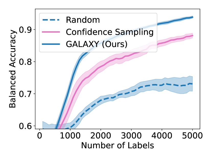
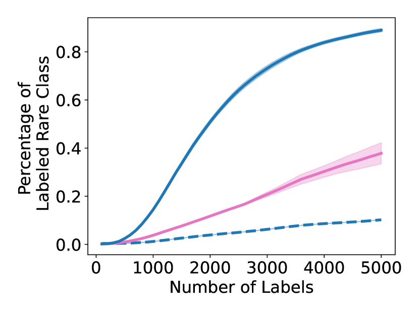
Unfortunately, under extreme class imbalance, uncertainty sampling tends to select examples mostly from the dominant class(es), often leading to very slow learning. In this paper, we take a novel approach specifically targeting the class imbalance problem. Our method is guaranteed to select examples that are both uncertain and class-diverse; i.e., the selected examples are relatively balanced across the classes even if the overall dataset is extremely unbalanced. In a nutshell, our algorithm sorts the examples by their softmax uncertainty scores and applies a bisection procedure to find consecutive pairs of points with differing labels. This procedure encourages finding uncertain points from a diverse set of classes. In contrast, uncertainty sampling focuses on sampling around the model’s decision boundary and therefore will collect a biased sample if this model decision boundary is strongly skewed towards one class. Figure 1 displays the results of one of our experiments, showing that our proposed GALAXY algorithm learns much more rapidly and collects a significantly more diverse dataset than uncertainty sampling.
We make the following contributions in this paper:
-
•
we develop a novel, scalable algorithm GALAXY, tailored to the extreme class imbalance setting, which is frequently encountered in practice,
-
•
GALAXY is easy to implement, requiring relatively simple modifications to commonplace uncertainty sampling approaches,
-
•
we conduct extensive experiments showing that GALAXY outperforms a wide collection of deep active learning algorithms in the imbalanced settings, and
-
•
we give a theoretical analysis showing that GALAXY selects much more class-balanced batches of uncertain examples than traditional uncertainty sampling strategies.
2 Related Work
Deep Active Learning: There are two main algorithmic approaches in deep active learning: uncertainty and diversity sampling. Uncertainty sampling queries the unlabeled examples that are most uncertain. Often, uncertainty is quantified by distance to the decision boundary of the current model (e.g., (Tong & Koller, 2001; Kremer et al., 2014; Balcan et al., 2009)). Several variants of uncertainty sampling have been proposed for deep learning (e.g., (Gal et al., 2017; Ducoffe & Precioso, 2018; Beluch et al., 2018).
In a batch setting, uncertainty sampling often leads to querying a set of very similar examples, giving much redundant information. To deal with this issue, diversity sampling queries a batch of diverse examples that are representative of the unlabeled pool. Sener & Savarese (2017) propose a Coreset approach for diversity sampling for deep learning. Others include (Gissin & Shalev-Shwartz, 2019; Geifman & El-Yaniv, 2017). However, under the class imbalance scenarios where collecting minority class examples is crucial, previous work by Coleman et al. (2020) has shown such methods to be less effective as they are expected to collect a subset with equal imbalance to the original dataset.
Recently, significant attention has been given to designing hybrid methods that query a batch of informative and diverse examples. Ash et al. (2019) balances uncertainty and diversity by representing each example by its last layer gradient and aiming to select a batch of examples with large Gram determinant. Citovsky et al. (2021) uses hierarchical agglomerative clustering to cluster the examples in the feature space and then cycles over the clusters querying the examples with smallest margin. Finally, Ash et al. (2021) uses experimental design to find a batch of diverse and uncertain examples.
Class Imbalance Deep Active Learning: A number of recent works have studied active learning in the presence of class imbalance. Coleman et al. (2020) proposes SEALS, a method for the setting of class imbalance and an enormous pool of unlabeled examples. Kothawade et al. (2021) proposes SIMILAR, which picks examples that are most similar with the collected in-distribution examples and most different from the known out-of-distribution examples. Their method achieves this by maximizing the conditional mutual information. Our setting is closest to their out-of-distribution imbalance scenario. Finally, Emam et al. (2021) tackles the class imablance issue by proposing BASE which queries the same number of examples per each predicted class based on margin from decision boundary, where the margin is defined by the distance to the model boundary in the feature space of the neural network.
By contrast with the above methods, our method searches adaptively in the output space within each batch for the best threshold separating two classes and provably produces a class-balanced set of labeled examples. Adaptively searching for the best threshold is especially helpful in the extreme class imbalance setting where the decision boundary of the model is often skewed. If all labels were known, theoretically it may be possible to modify the training algorithm to obtain a model without any skew towards on class. However, this is not possible in active learning where we do not know the labels a priori. In addition, it is expensive and undesirable in practical cases to modify the training algorithm (Roh et al., 2020), making it attractive to work for any off-the-shelf training algorithm (like ours).
Graph-based active learning: There have been a number of proposed graph-based adaptive learning algorithms (e.g., (Zhu et al., 2003a, b; Cesa-Bianchi et al., 2013; Gu & Han, 2012; Dasarathy et al., 2015; Kushnir & Venturi, 2020). Our work is most closely related to (Dasarathy et al., 2015), which proposed a graph-based active learning with strong theoretical guarantees. While assumes a graph as an input and will perform badly on difficult graphs, our work builds a framework that combines the ideas of with deep learning to perform active learning while continually improving the graph. We review this work in more detail in Section 4.
3 Problem Statement and Notation
We investigate the pool-based batched active learning setting, where the learner has access to a large pool of unlabeled data examples and there is an unknown ground truth label function giving the label of each example. At each iteration , the learner selects a small batch of unlabeled examples from the pool, observes its labels , and adds the examples to , the set of all the examples that have been labeled so far. After each batch of examples is queried, the learner updates the deep learning model training on all of the examples in and uses this model to inform which batch of examples are selected in the next round.
We are particularly interested in the extreme class imbalance problem where one class is significantly larger than the other classes. Mathematically,
where denote the number of examples that belong to the -th class. Here, is some small class imbalance factor and each of the in-distribution classes , …, contains far fewer examples than the out-of-distribution -th class. This models scenarios, for example in roof damage classification, self-driving and medical applications, in which a small fraction of the unlabeled examples are from classes of interest and the rest of the examples may be lumped into an “other” or “irrelevant” category.
Henceforth, we denote to be a model trained on the labeled set , where is a training algorithm that trains on a labeled set and outputs a classifier.
4 Review of Graph-based Active Learning
|
|
||
|
|
||
|
|
To begin, we introduce some notation. With slight abuse of notation, we define a undirected graph over the pool as with vertex set and edge set , where each node in the graph is also an example in the pool . Let denote the shortest path connecting and in the graph , and let denote its length.111In the special case when and are not connected, we define .
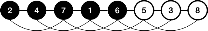
Dasarathy et al. (2015) proposed a graph-based active learning algorithm (see Algorithm 1) that aims to identify all the cuts , namely every edge that connects an oppositely labeled pair of examples. In particular, if one labeled all of the examples in the cut boundary , one would be able to classify every example in the pool correctly. As an example, take the linear graph in Figure 2(a) where each node represents a numbered example and is associated with a binary label (black/white). It is thus necessary to query at least seven examples to identify the cut boundary and therefore the labeling.
performs an alternating two phased procedure. First, if every pair of connected examples have the same label, queries an unlabeled example uniform at random. Second, whenever there exist paths connecting examples with different labels, the algorithm bisects along the shortest among these paths until it identifies a cut. The algorithm then removes the identified edge from the graph.
Dasarathy et al. (2015) has shown that the PAC sample complexity to identify all cuts highly depends on the input graph’s structural properties. As an example consider Figure 2, which depicts several graphs on the same set of examples. In graph (a), one needs to query at least seven examples, while in graph (b) one need only query two examples. Indeed, such a difference can be made arbitrarily large. The work of Dasarathy et al. (2015), however, did not address the major problem of how to obtain an “easier” graph that requires fewer examples queries for active learning.
5 GALAXY
Our algorithm GALAXY shown in Algorithm 4 blends graph-based active learning and deep active learning through the following two alternating steps
-
•
Given a trained neural network, we construct a graph based on the neural network’s predictions and apply a modified version of to it, efficiently collecting an informative batch of labels (Algorithm 4).
-
•
Given a new batch of labeled examples, we train a better neural network model that will be used to construct a better graph for active learning (Algorithm 2).
To construct graphs from a learned neural network in multi-class settings, we take a one-vs-all approach on the output (softmax) space as shown in Algorithm 2. For each class , we build a linear graph by ranking the model’s confidence margin on each example . For a neural network , the confidence margin is simply defined as , where denotes the -th element of the softmax vector. We break ties by the confidence scores themselves (equivalently by ). Intuitively, for each graph , we sort examples according to their likelihood to belong to class . Indeed, when is a perfect classifier on the pool, each linear graph constructed behaves like Figure 2(b), i.e., every example in class is perfectly separated from all other classes with only one cut in between.
Our algorithm GALAXY shown in Algorithm 4 proceeds in a batched style. For each batch, GALAXY first trains a neural network to obtain graphs constructed by the procedure described above. It then performs style bisection-like queries on all of the graphs but with two major differences.
-
•
To accommodate multiple graphs, we treat each linear graph as a binary one-vs-all graph, where we gather all shortest paths that connects a queried example in class and a queried example in any other classes. If such shortest paths exist, we then find the shortest of these shortest paths across all and the bisect the resulting shortest shortest path like in .
-
•
When no such shortest path exists, instead of querying an example uniform at random as in , we increase the order of the graphs by Algorithm 3 and perform bisection procedures on the updated graphs. Here, we refer to an -th order linear graph where each example is connected to all of its neighboring examples from each side. For example, Figure 2(c) shows a graph of order as opposed to an order graph shown in Figure 2(b). Intuitively, bisecting after the Connect procedure is equivalent with querying around the discovered cuts. For example in the case of Figure 2(b), after querying examples and , our algorithm will connect second order edges and query exactly examples and as the next two queries.
| (1) |
6 Analysis
|
|
||
|
|
6.1 GALAXY at the Extreme
In this section, we analyze the behavior of GALAXY in the two-class setting and specifically when class OOD (out-of-distribution) has much more examples than class ID (in-distribution). In a binary separable case, we bound expected batch balancedness of both the bisection procedure and GALAXY, whereas uncertainty sampling could fail to sample any ID examples at all. At the end we also show a noise tolerance guarantee that GALAXY will find the optimal uncertainty threshold with high probability. For proper indexing below, we let and .
Reduction to single linear graph. Recall in Algorithm 2, we build a graph for each class by sorting the margin scores of that class on the pool. In the binary classification case, it is sufficient to consider one graph generated from sorting confidence scores. This follows due to the symmetry of the two graphs in the binary case.
Universal approximator and region of uncertainty. Since neural networks are universal approximators, we make the following assumption.
Assumption 6.1.
Given a labeled subset of , let be the neural network classifier trained on . We assume classifies every example in perfectly. Namely, .
Definition 6.2.
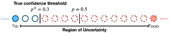
Let denote the labeled example in class ID with the highest confidence and denote the labeled example in class OOD with the lowest confidence. We then define all examples in between, i.e. , to be the region of uncertainty.
In practice, since the neural network model should be rather certain in its predictions on the labeled set, we expect the region of uncertainty to be relatively large. We show an example in Figure 3 where filled circles represent the labeled examples. The filled blue example on the left is and the filled red example on the right is . The region of uncertainty are then all of the examples in between.
In the following, we first derive our balancedness results in the separable case such as in Figure 3(a) and turn to noise tolerance analysis in the end. First in the separable case, we let denote the number of in-distribution examples and denote the number of out-of-distribution examples both in the region of uncertainty. First we analyze the bisection following procedure that adaptively finds the true uncertainty threshold (cut in the separable linear graph).
Definition 6.3.
Our bisection procedure works as follows when given region of uncertainty with examples.
-
•
Let represent the number of examples in the latest region of uncertainty, query the example based on the sorted uncertainty scores. Here, or with equal probability.
-
•
If observe ID, update the region of uncertainty to be examples ranked based on uncertainty scores. Recurse on the new region of uncertainty.
Similarly, if observe OOD, update the region of uncertainty to be examples ranked based on uncertainty scores. Recurse on the new region of uncertainty.
-
•
Terminate once the region of uncertainty is empty ().
The exact number of labels collected from the ID and OOD classes depends on the specific numbers of examples in the region of uncertainty. We characterize the generic behavior of the biscection process with a simple probabilistic model showing the following theorem that the method tends to find balanced examples among both classes. Proofs of the following results appear in the Appendices.
Theorem 6.4 (Sample Balancedness of Bisection).
Assume for some and that the examples labeled in the first bisection steps are all from class OOD. At least examples remain in the region of uncertainty and suppose that . If we let and be the number of queries in each of the ID and OOD classes made by the bisection procedure described in Definition 6.3, we must have
where the expectations are with respect to the uniform distribution above.
The unbalancedness factor of the region of uncertainty is at most . When is large, we must have . Thus, the bisection procedure collects a batch that improves on the unbalanced factor exponentially.
Next, we characterize the balancedness of the full GALAXY algorithm. When running GALAXY on a separable linear graph, it is equivalent with first running bisection procedure to find the optimal uncertainty threshold, followed by querying around the two sides of the threshold equally. We therefore incorporate our previous analysis on the bisection procedure and especially focus on the second part where one queries around the optimal uncertainty threshold.
Corollary 6.5 (Sample Balancedness of Batched GALAXY, Proof in Appendix B).
Assume and are under same noiseless setting as in Theorem 6.4. If GALAXY takes an additional queries after the bisection procedure terminates, so that examples are labeled in total and if we let and be the number of queries in each class made by GALAXY, we must have
where and the expectations are with respect to the uniform distribution in .
In the above theorem, since when is large, we can then recover a constant factor of balancedness. On the other hand, uncertainty sampling does not enjoy the same balancedness guarantees when the model decision boundary is biased towards the OOD class.
Proposition 6.6 (Sample Balancedness of Uncertainty Sampling).
Assume and are under same noiseless setting as in Theorem 6.4. If we let and be the number of queries in each of the ID and OOD classes made by an uncertainty sampling procedure with batch size steps, we have
where the expectations are with respect to . The minimization is taken over the true confidence threshold where the classification accuracy is maximized.
Note that the number of queries collected by uncertainty sampling, and , inherently depends on . The above proposition can been seen as demonstrated by Figure 3, where when training a model under extreme imbalance, the model could be biased towards OOD and thus the true confidence threshold . Since , in the worst case, uncertainty sampling could have selected a batch all in OOD regardless of the value takes. Therefore, in such cases, we have .
We will now show GALAXY’s robustness in non-separable graphs. We model the noises by randomly flipping the true labels of a separable graph.
Theorem 6.7 (Noise Tolerance of GALAXY, Proof in Appendix C).
Let . Suppose the true label of each example in the region of uncertainty is corrupted independently with probability . Let denote the batch size of GALAXY, and be the number of queries in each class made by GALAXY, with probability at least we have
where the expectations are with respect to .
Note in practice batch size in active learning is usually small. When , the above result also implies that with about labels corrupted at random, GALAXY collects a balanced batch with probability at least .
6.2 Time Complexity
We compare the per-batch running time of GALAXY with confidence sampling, showing that they are comparable in practice. Recall that is the batch size, is the pool size and is the number of classes. Let denote the forward inference time of a neural network on a single example.
Confidence sampling has running time , where comes from forward passes on the entire pool, comes from computing the maximum confidence of each example and is the time complexity of choosing the top-B examples according to uncertainty scores. On the other hand, our algorithm GALAXY has time . Here, is the complexity of constructing linear graphs (Algorithm 2) by sorting through margin scores and comes from finding the shortest shortest path, for elements among graphs.
In practice dominates all of the other terms, so making these running times comparable. Indeed, in all of our experiments conducted in Section 7.2, GALAXY is less than 5% slower when compared to confidence sampling.
7 Experiments
We conduct experiments under different class imbalance settings. These settings are generated from three image classification datasets with various class imbalance factors. If the classes are balanced in the dataset, then most active learning strategies (including GALAXY) perform similarly, with relative small differences in performance, so we focus our presentation on unbalanced situations. We will first describe the setups (Section 7.1) before turning to the results in Section 7.2. Finally, we present a comparison with vanilla algorithm and demonstrate the importance of reconstructing the graphs in Section 7.3.222Code can be found in https://github.com/jifanz/GALAXY.
7.1 Setup
We use the following metric and training algorithm to reweight each class by its number of examples. By doing this, we downweight significantly the large “other” class while not ignoring it completely. More formally, we state our metric and training objective below.
Metric: Given a fixed batch size and after iterations, let denote the labeled set after the final iteration. Let be a model trained on the labeled set. We wish to maximize the balanced accuracy over the pool
Recall that is the number of examples in class . In all of our experiments, we set and .
Remark 7.1.
Training Algorithm : Our training algorithm takes a labeled set as input. Let denote the number of labeled examples in class , we use a cross entropy loss weighted by for each class . Note unlike the evaluation metric, we do not directly reweight the classes by , as the active learning algorithms only have knowledge of labels of in practice. Furthermore for all experiments, we use the ResNet-18 model in PyTorch pretrained on ImageNet for initialization and cold-start the training for every labeled set . We use the Adam optimization algorithm with learning rate of and a fixed epochs for each .

7.2 Results on Extremely Unbalanced Datasets
We generate the extremely unbalanced settings for both binary and multi-class classification from popular vision datasets CIFAR-10(Krizhevsky et al., 2009), CIFAR-100(Krizhevsky et al., 2009), PathMNIST(Yang et al., 2021) and SVHN(Netzer et al., 2011). CIFAR-10 and SVHN both initially have 10 balanced classes while CIFAR-100 has balanced classes and PathMNIST has classes. In all of CIFAR-10, CIFAR-100 and SVHN, we construct the large “other” class by grouping the majority of the original classes into one out-of-distribution class. Suppose there are originally ( or ) balanced classes in the original dataset, we form a () class extremely unbalanced dataset by reusing classes as in the original dataset, whereas class contains all examples in classes in the original dataset. For PathMNIST, we consider the task of identifying cancer-associated stroma from the rest of hematoxylin & eosin stained histological images. Table 1 shows the detailed sizes of the extremely unbalanced datasets.
| Name | # Classes | |||
|---|---|---|---|---|
| CIFAR-10 | ||||
| CIFAR-10 | ||||
| CIFAR-100 | ||||
| CIFAR-100 | ||||
| CIFAR-100 | ||||
| SVHN | ||||
| SVHN | ||||
| PathMNIST |
Comparison Algorithms: We compare our algorithm GALAXY against eight baselines. SIMILAR (Kothawade et al., 2021), Cluster Margin (Citovsky et al., 2021), BASE (Emam et al., 2021), BADGE (Ash et al., 2019) and BAIT (Ash et al., 2021) have all been described in Section 2. For SIMILAR, we use the FLQMI relaxation of the submodular mutual information (SMI). We are unable to compare to the FLCMI relaxation of the submodular conditional mutual information (SCMI) due to excessively high memory usage required by the submodular maximization at pool size . As demonstrated in Kothawade et al. (2021) however, one should expect only marginal improvement over FLQMI relaxation of the SMI. For Cluster Margin we choose clustering hyperparameters so there are exactly clusters. We choose margin batch size to be while the target batch size is set to .
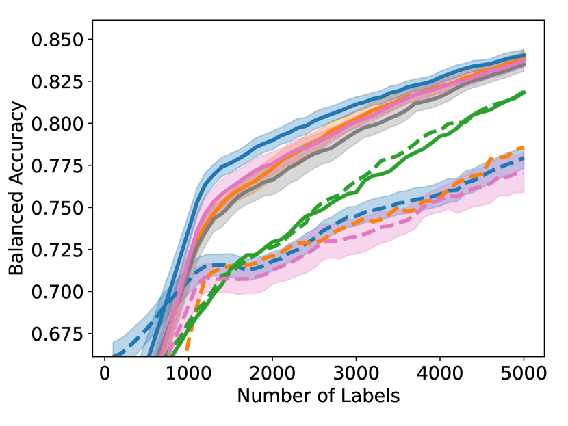
In addition to the above methods, Confidence Sampling (Settles, 2009) is a type of uncertainty sampling that queries the least confident examples in terms of . Here, is a classifier that outputs softmax scores and maximization is take with respect to classes. Most Likely Positive (Jiang et al., 2018; Warmuth et al., 2001, 2003) is a heuristic often used in active search, where the algorithm selects the examples most likely to be in the in-distribution classes by its predictive probabilities. Lastly, Random is the naive uniform random strategy. For each setting, we average over individual runs for each of GALAXY, Cluster Margin, BASE, Confidence Sampling, Most Likely Positive and Random. Due to computational constraints, we are only able to have single runs for each of SIMILAR, BADGE and BAIT. For algorithms with multiple runs, the standard error is also plotted as the confidence intervals. To demonstrate the active gains more clearly, all of our curves are smoothed by moving average with window size .
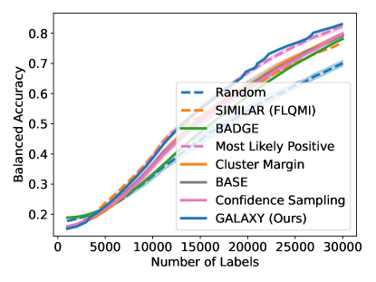
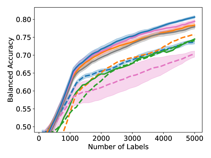
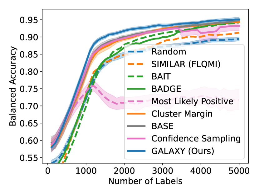
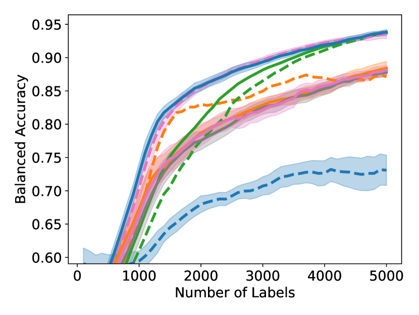
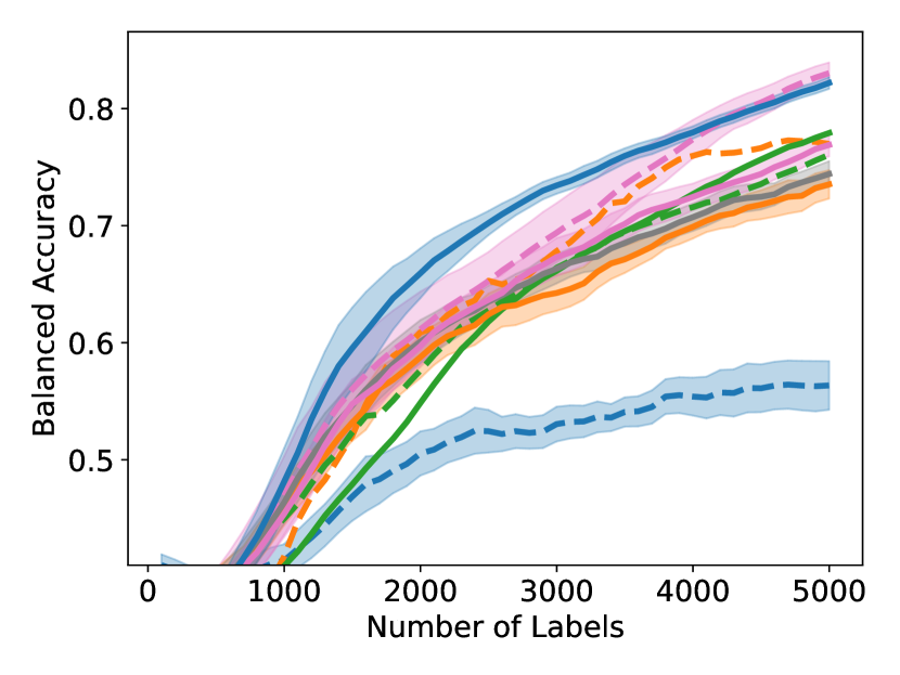
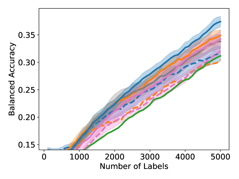
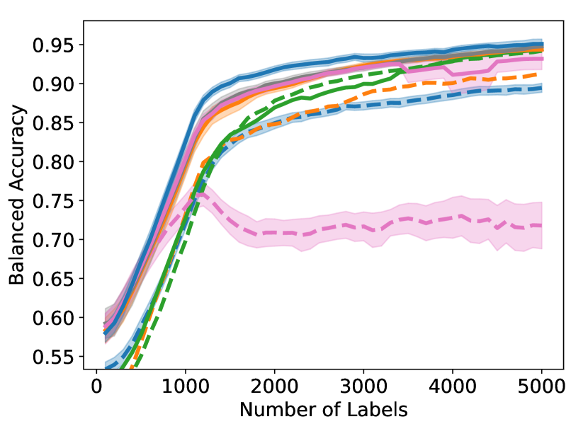
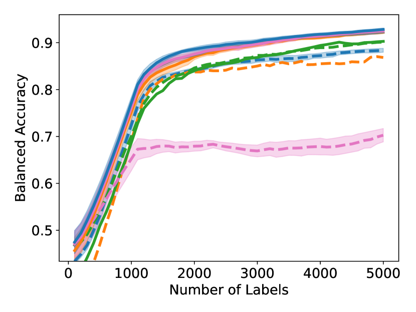
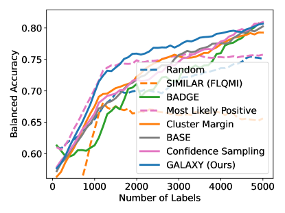
As shown in Figure 4, to achieve any balanced accuracy, GALAXY outperforms all baselines in terms of the number of labels requested, saving up to queries in some cases when comparing to the second best method. For example in unbalanced SVHN with 2 classes, to achieve , GALAXY takes queries while the second best algorithm takes queries. In unbalanced CIFAR-100 with 3 classes, to reach accuracy, GALAX takes queries while the second best algorithm takes queries. As expected, Cluster Margin and BASE are competitive in many settings as they also target unbalanced settings. BAIT and BADGE tend to perform less well primarily due to their focus on collecting data-diverse examples, which has roughly the same class-imbalance as the pool. Full experimental results on all settings are presented in Appendix D. In Appendix D, we also include an experiment on CIFAR-100, 10 classes with batch size showing the superiority of our method in the large budget regime.
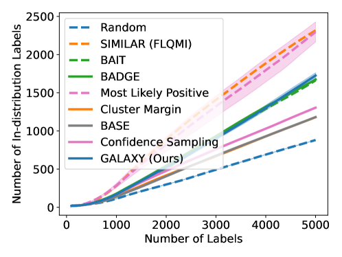
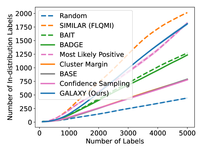
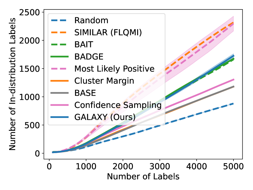
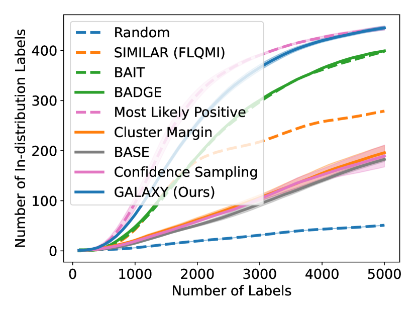
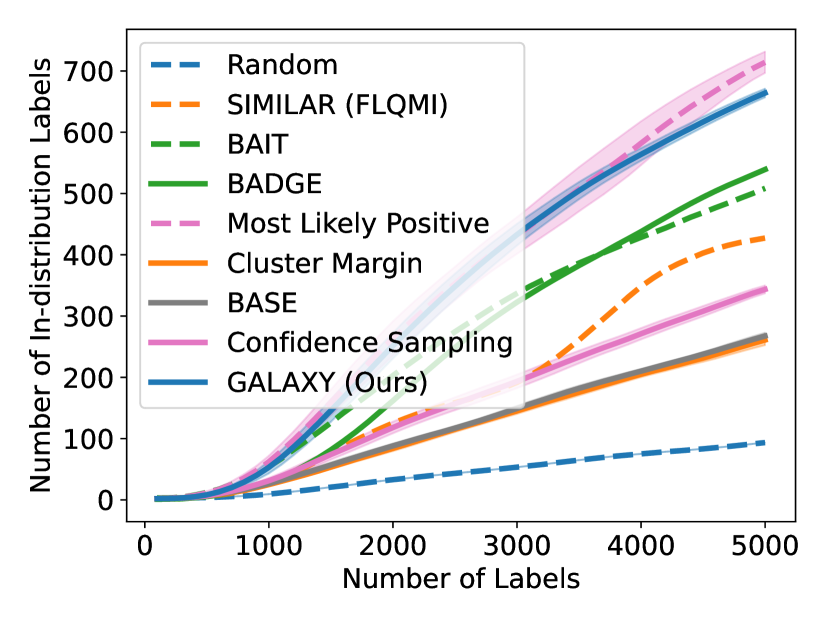
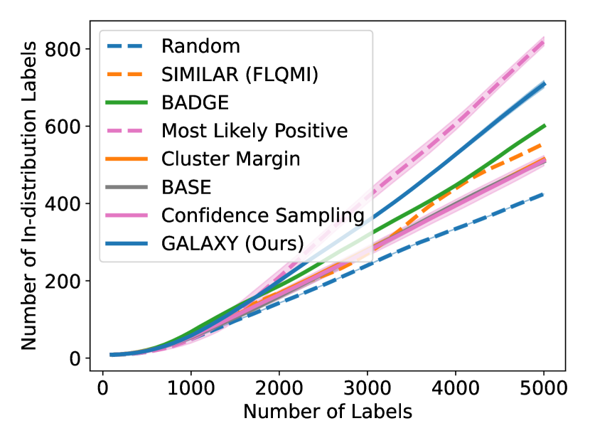
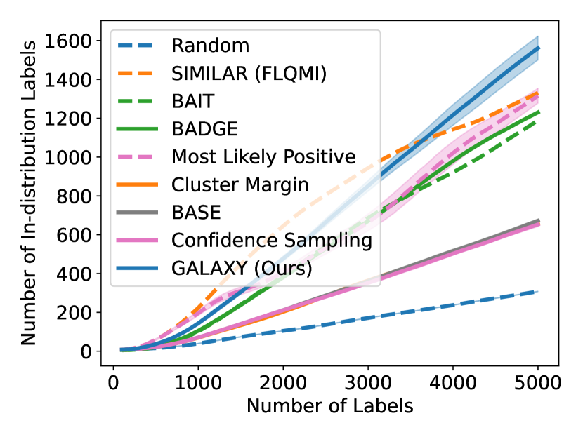
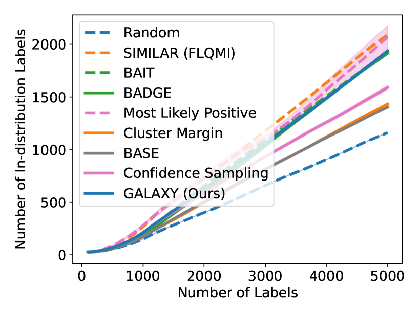
As shown in Figure 5, GALAXY’s success relies on its inherent feature of collecting a more balanced labeled set of uncertain examples. In particular, GALAXY is collecting a significantly more in-distribution examples than most baseline algorithms including uncertainty sampling. On the other hand, although SIMILAR and Most Likely Positive both collect more examples in the in-distribution classes, their inferiority in balanced accuracy suggests that the examples are not representative enough. Indeed, both methods are inherently collecting labels for example that are certain. This thus suggests the importance of collecting batches that are not only balanced but also uncertain.
7.3 Comparison: vs GALAXY
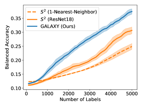
In this section, we conduct experiment to compare the original approach (Dasarathy et al., 2015) against our method. For , we construct a 10-nearest-neighbor graph from feature vectors of a ResNet-18 model pretrained on ImageNet. We show two curves of using two different models – 1-nearest-neighbor prediction on the graph and neural network training in Section 7.1. We note that the models training does not affect the active queries, whereas GALAXY constantly constructs graphs based on these updated models. As shown in Figure 6, GALAXY outperforms with both models by a significant margin, showing the necessity on learning and constructing better graphs (Algorithm 2).
8 Future Direction
In this paper, we propose a novel graph-based approach to deep active learning that particularly targets the extreme class imbalance cases. We show that our algorithm GALAXY outperforms all existing methods by collecting a mixture of balanced yet uncertain examples. GALAXY runs on similar time complexity as other uncertainty based methods by retraining the neural network model only after each batch. However, it still requires sequential and synchronous labelling within each batch. This means the human labelling effort cannot be parallelized by multiple annotators. For future work, we would like to incorporate asynchronous labelling and investigate its effect on our algorithm.
Acknowledgement
We thank Andrew Wagenmaker for insightful discussions. This work has been supported in part by NSF Award 2112471.
References
- Ash et al. (2019) Ash, J. T., Zhang, C., Krishnamurthy, A., Langford, J., and Agarwal, A. Deep batch active learning by diverse, uncertain gradient lower bounds. arXiv preprint arXiv:1906.03671, 2019.
- Ash et al. (2021) Ash, J. T., Goel, S., Krishnamurthy, A., and Kakade, S. Gone fishing: Neural active learning with fisher embeddings. arXiv preprint arXiv:2106.09675, 2021.
- Balcan et al. (2009) Balcan, M.-F., Beygelzimer, A., and Langford, J. Agnostic active learning. Journal of Computer and System Sciences, 75(1):78–89, 2009.
- Beluch et al. (2018) Beluch, W. H., Genewein, T., Nürnberger, A., and Köhler, J. M. The power of ensembles for active learning in image classification. In Proceedings of the IEEE Conference on Computer Vision and Pattern Recognition, pp. 9368–9377, 2018.
- Boucheron et al. (2005) Boucheron, S., Bousquet, O., and Lugosi, G. Theory of classification: A survey of some recent advances. ESAIM: probability and statistics, 9:323–375, 2005.
- Cesa-Bianchi et al. (2013) Cesa-Bianchi, N., Gentile, C., Vitale, F., and Zappella, G. Active learning on trees and graphs. arXiv preprint arXiv:1301.5112, 2013.
- Citovsky et al. (2021) Citovsky, G., DeSalvo, G., Gentile, C., Karydas, L., Rajagopalan, A., Rostamizadeh, A., and Kumar, S. Batch active learning at scale. Advances in Neural Information Processing Systems, 34, 2021.
- Coleman et al. (2020) Coleman, C., Chou, E., Katz-Samuels, J., Culatana, S., Bailis, P., Berg, A. C., Nowak, R., Sumbaly, R., Zaharia, M., and Yalniz, I. Z. Similarity search for efficient active learning and search of rare concepts. arXiv preprint arXiv:2007.00077, 2020.
- Conathan et al. (2018) Conathan, D., Oswal, U., and Nowak, R. Active sparse feature selection using deep convolutional features for image retrieval. SIAM International Conference on Data Mining. First workshop on AI in insurance., 2018. URL https://www.ai-ml-amfam.com/_files/ugd/bf4274_dcb4dbffea374bc9b62abca6a51573d2.pdf.
- Dasarathy et al. (2015) Dasarathy, G., Nowak, R., and Zhu, X. S2: An efficient graph based active learning algorithm with application to nonparametric classification. In Conference on Learning Theory, pp. 503–522. PMLR, 2015.
- Ducoffe & Precioso (2018) Ducoffe, M. and Precioso, F. Adversarial active learning for deep networks: a margin based approach. arXiv preprint arXiv:1802.09841, 2018.
- Emam et al. (2021) Emam, Z. A. S., Chu, H.-M., Chiang, P.-Y., Czaja, W., Leapman, R., Goldblum, M., and Goldstein, T. Active learning at the imagenet scale. arXiv preprint arXiv:2111.12880, 2021.
- Gal et al. (2017) Gal, Y., Islam, R., and Ghahramani, Z. Deep bayesian active learning with image data. In International Conference on Machine Learning, pp. 1183–1192. PMLR, 2017.
- Geifman & El-Yaniv (2017) Geifman, Y. and El-Yaniv, R. Deep active learning over the long tail. arXiv preprint arXiv:1711.00941, 2017.
- Gissin & Shalev-Shwartz (2019) Gissin, D. and Shalev-Shwartz, S. Discriminative active learning. arXiv preprint arXiv:1907.06347, 2019.
- Gu & Han (2012) Gu, Q. and Han, J. Towards active learning on graphs: An error bound minimization approach. In 2012 IEEE 12th International Conference on Data Mining, pp. 882–887. IEEE, 2012.
- Jiang et al. (2018) Jiang, S., Malkomes, G., Abbott, M., Moseley, B., and Garnett, R. Efficient nonmyopic batch active search. In 32nd Conference on Neural Information Processing Systems (NeurIPS 2018), 2018.
- Katz-Samuels et al. (2021) Katz-Samuels, J., Zhang, J., Jain, L., and Jamieson, K. Improved algorithms for agnostic pool-based active classification. arXiv preprint arXiv:2105.06499, 2021.
- Kothawade et al. (2021) Kothawade, S., Beck, N., Killamsetty, K., and Iyer, R. Similar: Submodular information measures based active learning in realistic scenarios. Advances in Neural Information Processing Systems, 34, 2021.
- Kremer et al. (2014) Kremer, J., Steenstrup Pedersen, K., and Igel, C. Active learning with support vector machines. Wiley Interdisciplinary Reviews: Data Mining and Knowledge Discovery, 4(4):313–326, 2014.
- Krizhevsky et al. (2009) Krizhevsky, A., Hinton, G., et al. Learning multiple layers of features from tiny images. 2009.
- Kushnir & Venturi (2020) Kushnir, D. and Venturi, L. Diffusion-based deep active learning. arXiv preprint arXiv:2003.10339, 2020.
- Netzer et al. (2011) Netzer, Y., Wang, T., Coates, A., Bissacco, A., Wu, B., and Ng, A. Y. Reading digits in natural images with unsupervised feature learning. 2011.
- Roh et al. (2020) Roh, Y., Lee, K., Whang, S. E., and Suh, C. Fairbatch: Batch selection for model fairness. arXiv preprint arXiv:2012.01696, 2020.
- Sener & Savarese (2017) Sener, O. and Savarese, S. Active learning for convolutional neural networks: A core-set approach. arXiv preprint arXiv:1708.00489, 2017.
- Settles (2009) Settles, B. Active learning literature survey. 2009.
- Tong & Koller (2001) Tong, S. and Koller, D. Support vector machine active learning with applications to text classification. Journal of machine learning research, 2(Nov):45–66, 2001.
- Warmuth et al. (2001) Warmuth, M. K., Rätsch, G., Mathieson, M., Liao, J., and Lemmen, C. Active learning in the drug discovery process. In NIPS, pp. 1449–1456, 2001.
- Warmuth et al. (2003) Warmuth, M. K., Liao, J., Rätsch, G., Mathieson, M., Putta, S., and Lemmen, C. Active learning with support vector machines in the drug discovery process. Journal of chemical information and computer sciences, 43(2):667–673, 2003.
- Yang et al. (2021) Yang, J., Shi, R., Wei, D., Liu, Z., Zhao, L., Ke, B., Pfister, H., and Ni, B. Medmnist v2: A large-scale lightweight benchmark for 2d and 3d biomedical image classification. arXiv preprint arXiv:2110.14795, 2021.
- Zhu et al. (2003a) Zhu, X., Ghahramani, Z., and Lafferty, J. D. Semi-supervised learning using gaussian fields and harmonic functions. In Proceedings of the 20th International conference on Machine learning (ICML-03), pp. 912–919, 2003a.
- Zhu et al. (2003b) Zhu, X., Lafferty, J., and Ghahramani, Z. Combining active learning and semi-supervised learning using gaussian fields and harmonic functions. In ICML 2003 workshop on the continuum from labeled to unlabeled data in machine learning and data mining, volume 3, 2003b.
Appendix A Proof of Theorem 6.4
Proof.
First, when , it’s easy to see by induction that after queries, the region of uncertainty shrinks to have at least examples. Therefore, after steps, we must have .
Next, let denote the number of OOD labels queried after bisecting steps, namely . Since in the last examples, the number of ID examples is , we must have the number of OOD examples to be symmetrically . Therefore, due to symmetry of distribution and the bisection procedure, in expectation the bisection procedure queries equal numbers of ID and OOD examples, i.e. . Together we must have
where the last inequality follows from the total number of queries so . ∎
Appendix B Proof of Corollary 6.5
Proof.
As shown in Theorem 6.4, even without the additional queries, we must have . Now, for the process of querying two sides of the cut, with queries we can guarantee that at least examples to the left of the cut must have been queried and are in ID. Therefore, . As a result, we the have and , so
∎
Appendix C Proof of Theorem 6.7
Lemma C.1 (Noise Tolerance of Bisection).
Let . If the true label of each example in the region of uncertainty is corrupted independently with probability , the bisection procedure recovers the true uncertainty threshold with probability at least .
Proof.
Bisection procedure will make queries and for each query the label could be corrupted with probability . Therefore, by union bound, we must then have
∎
Now we start to prove Theorem 6.7.
Appendix D Full Experimental Results on CIFAR-10, CIFAR-100 and SVHN

D.1 Large-budget Regime
In Figure 15, we use a batch size and average over runs. We use a labelling budget of out of the pool of size . Note that confidence sampling performs competitive in this case but could fail catastrophically in cases such as SVHN, 3 classes.