Gap solitons in elongated geometries: the one-dimensional Gross-Pitaevskii equation and beyond
Abstract
We report results of a systematic analysis of matter-wave gap solitons (GSs) in three-dimensional self-repulsive Bose-Einstein condensates (BECs) loaded into a combination of a cigar-shaped trap and axial optical-lattice (OL) potential. Basic cases of the strong, intermediate, and weak radial (transverse) confinement are considered, as well as settings with shallow and deep OL potentials. Only in the case of the shallow lattice combined with tight radial confinement, which actually has little relevance to realistic experimental conditions, does the usual one-dimensional (1D) cubic Gross-Pitaevskii equation (GPE) furnish a sufficiently accurate description of GSs. However, the effective 1D equation with the nonpolynomial nonlinearity, derived in Ref. [Phys. Rev. A 77, 013617 (2008)], provides for quite an accurate approximation for the GSs in all cases, including the situation with weak transverse confinement, when the soliton’s shape includes a considerable contribution from higher-order transverse modes, in addition to the usual ground-state wave function of the respective harmonic oscillator. Both fundamental GSs and their multipeak bound states are considered. The stability is analyzed by means of systematic simulations. It is concluded that almost all the fundamental GSs are stable, while their bound states may be stable if the underlying OL potential is deep enough.
pacs:
03.75.Lm, 05.45.YvI INTRODUCTION
Matter-wave gap solitons (GSs) are localized modes that can be created in elongated Bose-Einstein condensates (BECs) loaded into one-dimensional (1D) optical-lattice (OL) potentials, with the intrinsic nonlinearity induced by repulsive interactions between atoms. GSs have been the topic of a large number of original works. Results produced by these studies were summarized in several reviews Kon1 ; Mor1 ; Carre1 ; Carre2 ; Barcelona . Within the framework of the mean-field approximation, the description of matter-wave patterns is based on the Gross-Pitaevskii equation (GPE) for the macroscopic wave function GPE :
| (1) |
which has proven to be very successful in reproducing experimental results for the zero-temperature BEC (for instance, for multiple vortices, as shown in detail in Refs. Vort ; Huht ). In this equation, is the atomic mass, the norm of the wave function is unity, is the number of atoms, and is the interaction strength with being the s-wave scattering length. In this work, we consider only repulsive interactions (i.e., ). Furthermore, is the radial-confinement potential and is the axial potential, which may include the axial harmonic trap and the 1D OL, with depth and period :
| (2) |
The energy scale in the underlying (no-interaction) linear problem is set by the OL’s recoil energy, .
Most commonly, theoretical studies of GSs in elongated geometries are carried out in terms of the 1D GPE Kon1 ; Mor1 ; Kiv1 ; Abd1 ; Mal1 ; Wu1 ; Wu2 :
| (3) |
where . This is an effective evolution equation for the axial dynamics —described by the 1D wave function — which can be derived from the full three-dimensional (3D) GPE after averaging out the radial degrees of freedom under the assumption that the radial confinement is so tight that the transverse dynamics are frozen to zero-point oscillations. These conditions, however, are not easy to realize using typical experimental parameters Mor1 , and when such conditions are not met the transverse excitations can no longer be neglected, making an essentially 3D analysis necessary. In this work, we aim to investigate different physically relevant regimes and capture 3D effects in the generation and stability of matter-wave GSs in elongated BECs. This analysis should make it possible to determine the range of validity of the 1D GPE for the description of the GSs under typical experimental conditions, as well as characteristic features of the fundamental and higher-order GSs in realistic situations.
In principle, when the transverse excitations are relevant, Eq. (3) fails and one has to resort to the full 3D GPE (1), as recently done in Ref. PRA82 , or, alternatively, use extended 1D models that, within the framework of certain assumptions, take into account effects of higher-order radial modes on the axial dynamics of the condensate, leading to effective 1D equations with the cubic-quintic CQ or nonpolynomial Reatto1 ; PRA77 nonlinearities. In this work, we will consider both the full 3D GPE and the effective 1D model with a nonpolynomial nonlinearity, which was derived, for the case of the self-repulsive nonlinearity, in Ref. PRA77 . The latter one, which represents a simple generalization of the usual 1D GPE, that reduces to Eq. (3) in the appropriate limit, has demonstrated an excellent quantitative agreement with experimental observations Kev1 ; Wel1 ; Kev2 ; Carre3 (chiefly, for delocalized dark solitons, which are natural patterns in the case of the self-repulsion; however, the comparison was not reported before for localized GS modes). We will demonstrate that, while the range of applicability of the 1D GPE (3) is severely limited in realistic situations, the above-mentioned generalization gives a good description of stationary matter-wave GSs in virtually all cases of practical interest.
The paper is organized as follows. The model is formulated in Section II, where we also recapitulate the derivation of the effective nonpolynomial 1D equation following the lines of Ref. PRA77 , as this derivation is essential for the presentation of the results for the GSs. The main findings are collected in Sections III, where families of GS solutions are reported in several physically relevant regimes for strong, intermediate, and weak transverse confinement and shallow or deep OL potential. Both fundamental GSs and their multipeak bound states are considered. Only in the case of tight confinement combined with a shallow OL does the ordinary 1D GPE provide for a sufficiently accurate description of the GSs in comparison with results of full 3D computations. On the other hand, the effective nonpolynomial 1D equation provides for good accuracy in all cases; for the fundamental solitons and their bound states alike. The stability of the GSs is studied in Section IV by means of systematic simulations of the evolution of perturbed solitons. The conclusion is that the fundamental GSs are stable (except in a narrow region close to the upper edge of the band gaps), even in the case of strong deviation from the usual 1D description. Multisoliton bound states are stable if the OL potential is deep enough. Conclusions following from results of this work, including applicability limits for the mean-field approximation and 1D approximations, are formulated in Section V.
II THE MODEL
The model that was developed in Ref. PRA77 for a BEC in the absence of OL potentials resorted to the adiabatic approximation, to neglect correlations between the transverse and axial motions. This approximation assumes that the axial density varies slowly enough to allow the transverse wave function to follow these slow variations. Because the OL imposes a new spatial scale, which may be more restrictive, it is necessary to find out if the adiabatic approximation remains valid in the presence of the OL. To this end, we will now briefly recapitulate the derivation of the effective 1D equation based on this approximation.
The starting point is the ansatz based on the factorized 3D wave function
| (4) |
with being the local condensate density per unit length characterizing the axial configuration:
| (5) |
To derive Eq. (5), we have assumed that the transverse wave function is normalized to unity. Next, the substitution of Eq. (4) into the 3D equation (1) leads to
| (6) |
Because of the very different time scales of the axial and radial motions, it is natural to assume that the slow axial dynamics may be accurately described by averaging Eq. (6) over the fast (radial) degrees of freedom. Doing this, one obtains
| (7) |
| (8) |
Since enters the last term of Eq. (8) merely as an external parameter, it is clear that, whenever the axial kinetic energy associated with the transverse wave function may be neglected; namely,
| (9) |
the radial dynamics decouple and can be determined without the knowledge of the axial wave function. Actually, the right-hand side of Eq. (9) is the chemical potential of an axially homogeneous condensate characterized by the density per unit length and wave function . For a sufficiently small value of the linear density (), the chemical potential of the lowest-energy state of this homogeneous condensate can be readily obtained perturbatively. In this case, to the lowest order, is given by the Gaussian wave function of the ground state of the radial harmonic oscillator, with the corresponding chemical potential being . As the linear density increases, more radial modes become excited and, in general, the ground state of the corresponding homogeneous condensate involves many harmonic-oscillator modes.
In previous works, it was shown using different approaches that, also in this case, an analytical solution can be constructed PRA77 . In particular, by using a variational approach based on the direct minimization of the chemical-potential functional, it was shown that, for any (dimensionless) linear density , a very accurate estimate for the chemical potential of the ground state is given by Ger1 . This expression can be easily extended to incorporate the case in which the condensate contains an axisymmetric vortex PRA77 (see also Ref. Luca , where the intrinsic vorticity was included into the derivation of the 1D nonpolynomial nonlinear Schrödinger equation in the case of self-attraction). However, in this work we restrict the consideration to zero vorticity. Using Eq. (9), we see that a sufficient condition for the second derivative in appearing in Eq. (8) to be negligible is
| (10) |
Taking into account an estimate, , where is the characteristic length scale in the axial direction, Eq. (10) can be rewritten as
| (11) |
When this condition holds, coincides, to a good approximation, with the transverse local chemical potential of the stationary radial GPE:
| (12) |
and is given by
| (13) |
Finally, substituting Eqs. (13) and (5) into Eq. (7) and taking into account that is a real normalized wave function (which implies the vanishing of the integral in the last term), we arrive at the following effective 1D equation to govern the slow axial dynamics of the condensate:
| (14) |
We note that the contribution from interatomic interactions enters the above equation through term , which vanishes for . Thus, Eq. (14) incorporates an energy shift , which is irrelevant for the dynamics but simplifies the form of the equation and makes the global chemical potential that follows from this effective 1D equation exactly coinciding with the corresponding 3D result.
The above derivation demonstrates that the validity of Eq. (14) relies on two conditions:
(i) The typical time scale of the axial motion must be much larger than the typical time scale of the radial motion ().
(ii) The axial kinetic energy associated with the transverse wave function must be negligible.
The former requirement is necessary to allow the radial wave function to adiabatically follow the axial dynamics. While the specific temporal scale depends on the particular initial conditions, typically, in the presence of an OL, the fulfillment of this condition gets more difficult as the lattice period decreases, or the linear density increases. In particular, a sufficient condition for the validity of the adiabatic approximation is: , , with being the radial harmonic-oscillator length. Nevertheless, such a constraint, which is hard to satisfy in realistic situations, is not a necessary condition. Actually, for stationary states and condition (i) always holds. In the present work we are interested in this case, which is the most relevant one to seek for matter-wave GSs.
A sufficient condition for the fulfillment of condition (ii) is given by the inequality (11). In the presence of an OL, the characteristic length scale is typically on the order of the lattice period , hence Eq. (11) becomes
| (15) |
where is the corresponding recoil energy. We will demonstrate that this condition is well satisfied for stationary GSs in most cases of interest.
It is clear that, when the linear density is small enough (), Eq. (14), which exhibits the nonpolynomial nonlinearity, reduces to the usual 1D GPE (3) with the cubic nonlinearity. This is the quasi-1D mean-field regime, which corresponds to condensates whose radial state, as given by a solution to Eq. (12), may be well approximated by the Gaussian ground state of the corresponding harmonic oscillator PRA77 ; PRA74 . Thus, Eq. (14) represents an extension of the 1D GPE for condensates with larger linear densities or, equivalently, larger mean-field interaction energies. In such condensates, the radial ground state satisfying Eq. (12) is, in general, a linear combination of many harmonic-oscillator modes (a similar situation takes place in the derivation of the effective 1D equation for fermionic gases by means of the density-functional approach SKA ).
Inspection of Eqs. (1) or (14) demonstrates that the dynamical problem is fully controlled by four dimensionless parameters, which may be defined as
| (16) |
As said above, the recoil energy sets the energy scale of the underlying linear problem, while the nonlinear coupling constant determines the order of magnitude of the mean-field interaction energy in units of the radial quantum . Note that the dimensionless linear density is proportional to .
In this work, we assume the axial confinement to be so weak that the corresponding harmonic-oscillator length, , is much larger than the lattice period . Under these conditions, it is safe to neglect the modulation induced in the condensate density by the axial harmonic trap and set , so that we are left with a uniform 1D lattice potential acting along the axial direction.
III MATTER-WAVE GAP SOLITONS IN DIFFERENT PHYSICAL REGIMES
The stationary solutions of the 3D GPE are wave functions of the form , with obeying the time-independent GPE:
| (17) |
where is the chemical potential. When Eq. (14) is applicable, one can instead generate the stationary axial wave function by solving the effective 1D equation
| (18) |
which, in the limit of , reduces to the time-independent version of the usual 1D GPE (3):
| (19) |
Matter-wave GSs are characterized by a chemical potential lying in a band gap of the energy spectrum of the underlying linear system. To construct solutions for realistic 3D matter-wave GSs in the effectively 1D geometry, we looked for numerical solutions to Eqs. (17) and (18) in different physically relevant regimes, and compared the obtained results with those produced by the usual 1D GPE (19) to determine to what extent 3D contributions are relevant. In particular, the comparison allows us to estimate the accuracy and range of applicability of the effective 1D equations (18) and (19).
Experimentally relevant values for the OL period range from to Mor1 , which implies that, for the condensate of 87Rb, ranges from to . Taking into account that, typically, , we conclude that . On the other hand, for the condensate of 23Na one has Na ; therefore, in this case the GS energy is sufficiently large to excite higher modes of the radial confinement, which makes 3D contributions always relevant. Since the 87Rb condensate is most relevant for the experimental realization of GSs in the quasi-1D setting Ober1 ; Isa1 , in what follows below we use particular parameters of this condensate to illustrate our results. Nevertheless, the results of the present work, which are always expressed in terms of relevant dimensionless parameters, are valid for any BEC. Actually, this is a direct consequence of the scaling properties of Eqs. (1), (3), and (14).
III.1 Tight radial confinement:
In this case, the quantum of radial excitations is much greater than the typical energy scale in the linear problem. Note that, to realize this regime in a 87Rb condensate, even in an OL of period , one needs to use a harmonic trap with radial frequency .
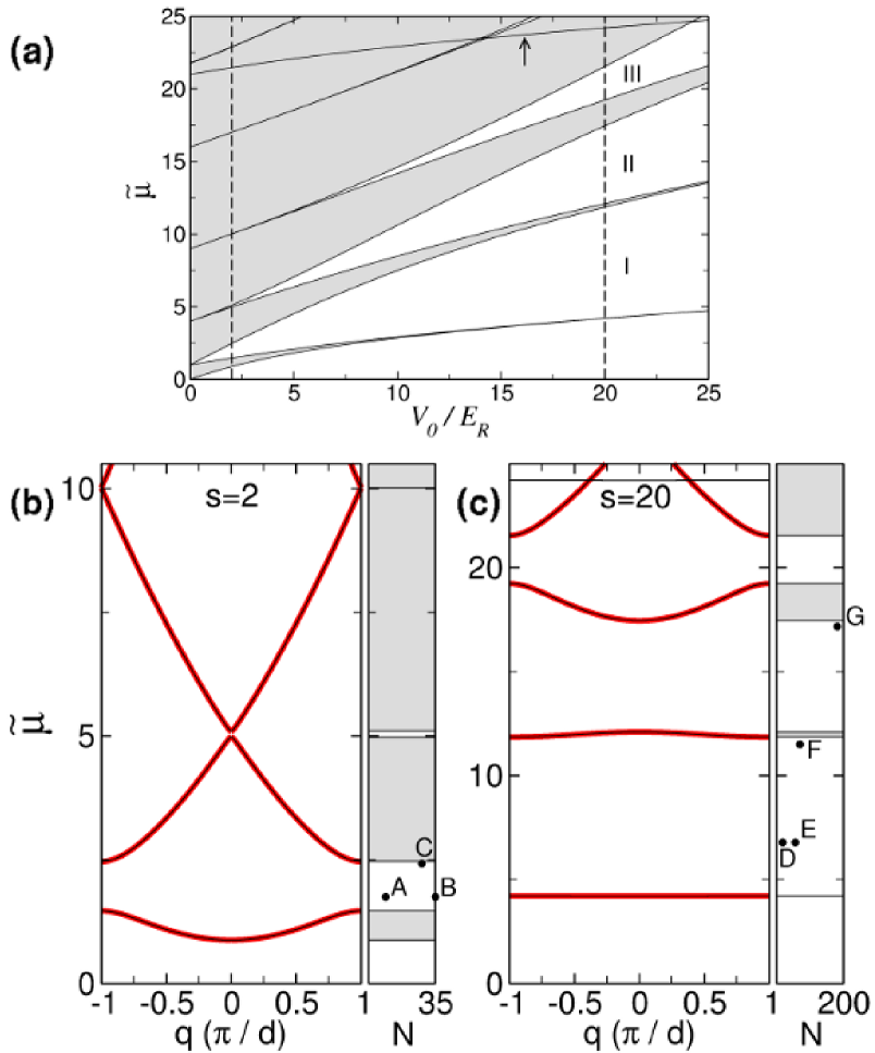
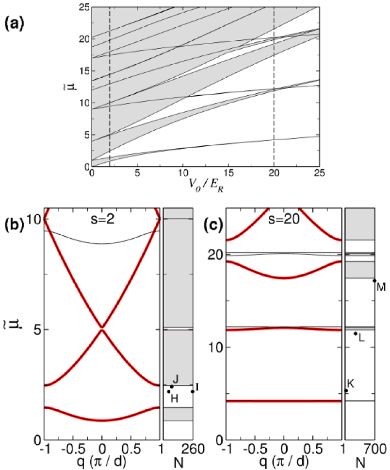
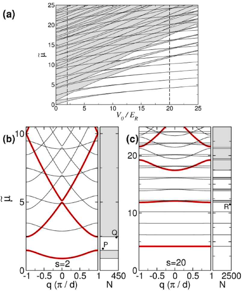
Figure 1(a) shows the dimensionless chemical potential of the noninteracting 3D condensate with ,
| (20) |
as a function of the dimensionless lattice depth, . Since in this work we are interested in GSs with zero vorticity, this diagram, which represents the band-gap structure of the underlying linear problem, has been obtained from the zero-vorticity solutions of the linear version of Eq. (17). Regions I, II, and III correspond to the lowest finite band gaps, which separate shaded bands, where linear solutions exist. An important point is that, within the region of interest in the parameter space (for and up to the third band gap), this 3D diagram is indistinguishable from that obtained using the linear version of the effective 1D equation (18) [which, obviously, coincides with the linear version of the stationary 1D GPE (19)]. In fact, Eq. (18) leads to a band-gap diagram that differs from Fig. 1(a) solely in the band marked by the arrow, which does not appear in the 1D case. This extra band is, essentially, a replica of the lowest one, shifted up in energy by . Taking into account that the energy spectrum of the radial harmonic oscillator is given by
| (21) |
where is the radial quantum number and is the axial angular-momentum quantum number, it is evident that the additional up-shifted band corresponds to the first-excited radial mode with . In the notation of Ref. PRA82 , it corresponds to quantum numbers , with being the band index of the 1D axial problem. Thus, the appearance of this band is a purely 3D effect that cannot be accounted for by the above 1D models. Since the energy shift increases as decreases, it is clear that, within the parameter region of interest, Fig. 1(a) is universal in the sense that it is valid (for both 1D and 3D systems) for any .
In this work, we restrict ourselves to the case of GSs; that is, the solitons bifurcating from the lowest-energy band. Three-dimensional matter-wave GSs with a nontrivial radial structure have been studied in Ref. PRA82 . In this subsection, we consider OLs with and depth or . These two representative cases correspond to the dashed vertical lines in Fig. 1(a) and are shown in more detail in Figs. 1(b) and 1(c), which display the corresponding band-gap structure as a function of the quasimomentum in the first Brillouin zone (in units of ). Bold red lines in Figs. 1(b) and 1(c) have been obtained from the linear version of the effective 1D equation (18) while thin black lines correspond to results obtained by means of the linear version of the 3D equation (17) that cannot be reproduced with the 1D model. As mentioned above, the only appreciable difference between the 1D and 3D results comes from the contribution of the first-excited radial mode [see the top part of Fig. 1(c)]. The case of , displayed in Fig. 1(b), corresponds to the condensate in relatively shallow OL potentials. Under these circumstances, the linear energy spectrum does not differ too much from that corresponding to the translationally invariant case (), and the band-gap structure exhibits wide energy bands separated by relatively small gaps, which are tangible only in the lowest part of the spectrum. On the contrary, for [the tight-binding regime, see Fig. 1(c)] the condensate is trapped in the deep periodic potential. In this case, the lowest part of the linear spectrum is dominated by large gaps separating relatively narrow energy bands. The panels on the right side of Figs. 1(b) and 1(c) show the location, with respect to the corresponding linear band-gap diagram, of the GSs that will be considered below (points A–G). The horizontal axes in these panels indicate the number of atoms in each GS for the 87Rb condensates (with the s-wave scattering length ) in the trap with radial frequency . For other parameter values, the GS family is described by the same plots, if considered in terms of the above-mentioned nonlinear coupling constant, [ and correspond to ]. In other words, the number of atoms in a GS created in the condensate with scattering length and transverse confinement radius , which is tantamount to the GS with particular values of , and , is given by
| (22) |
GS solutions have been obtained by numerically solving the full 3D equation (17), as well as the effective 1D equations (18) and (19). To this end, we have implemented a Newton continuation method, based on a Laguerre–Fourier spectral basis, that uses the chemical potential as a continuation parameter. To ensure the convergence, methods of this kind require initiation of the iterative procedure with a sufficiently good initial guess. This means that one needs a good estimate for both the axial and the radial parts of the wave function. Our computations used the following initial ansatz for the wave function:
| (23) |
where the -dependent condensate’s width, expressed in units of , is
| (24) |
and is the axial wave function. The number of particles, , and are free adjustable parameters. Note that the radial part of the wave function (23) is the same as the variational solution of Eq. (12), which was found in Ref. PRA77 .
III.1.1 Shallow optical lattice:
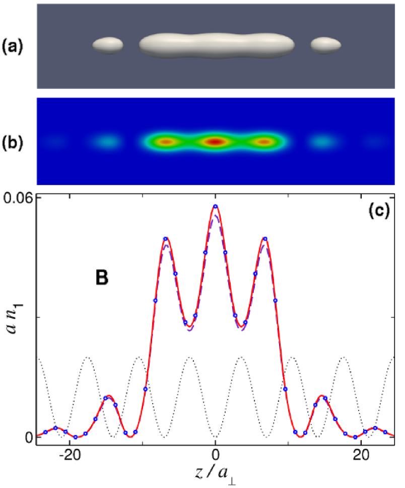
Point A in Fig. 1(b) corresponds to a fundamental GS located near the bottom edge of the first band gap. It looks qualitatively similar to that shown below in Fig. 3, but with the peak linear density . In this case, the effective 1D equations (18) and (19) yield results which are indistinguishable, on the scale of the figures, from those obtained from the full 3D equation (17). This is not surprising because, for these parameters, condition (15) is certainly satisfied, and inequality , which guarantees the validity of the 1D GPE (19), also holds. The (dimensionless) chemical potential of this GS is , which implies , hence the radial wave function of the condensate should not differ too much from the ground state of the corresponding harmonic oscillator. These fundamental GSs, however, can only accommodate particles (for the 87Rb condensate), which is too small to use the mean-field approximation. Yet these solutions play an important role as building blocks of higher-order GSs. Point B in Fig. 1(b) corresponds to one of these higher-order solitons, which is built as a symmetric linear combination of three fundamental GSs, see Fig. 2. Its chemical potential and number of particles are and . Note that, for the relatively shallow OL (), interference effects arising from the overlap between fundamental GSs sitting in adjacent lattice cells play an important role. For this reason, the contrast between the three central peaks and minima separating them is rather low in Fig. 2, and the total number of particles in the compound soliton does not coincide with the sum of the numbers of its fundamental constituents. Extending this procedure, one can readily build a sequence of compound GSs with an increasing number of peaks.
Panels (a) and (b) in Fig. 2 display the 3D density of the three-peak GSs as, respectively, an isosurface (taken at of the maximum density) and a color map in the cross-section plane drawn through the axis. From these results, which have been obtained by solving the full 3D equation (17), we have also derived the axial linear density , defined as per Eq. (5). This density is shown in Fig. 2(c) by open circles, along with the corresponding results obtained from the effective 1D equations (18) and (19). The OL potential is also displayed by the dotted line (in arbitrary units). It is seen that the effective 1D equation (18) (solid red lines) reproduces the 3D results very accurately. The 1D GPE (19) (dashed blue lines) gives a slight discrepancy () against the 3D results. This discrepancy, which would be invisible in the isolated fundamental GSs that build the compound, may also be explained by effects of the interference between the constituents.
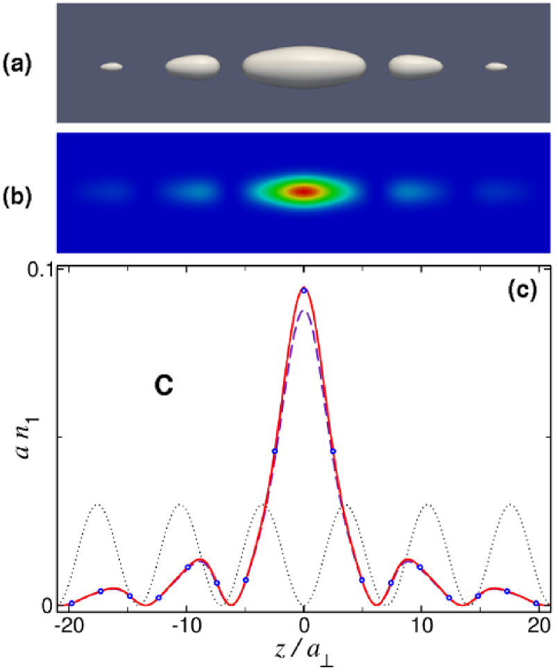
Point C in Fig. 1(b) indicates the location of a fundamental gap soliton in the plane, which sits near the top edge of the first band gap. It contains particles and has chemical potential , which corresponds to . This quantity is again very similar to , so that one expects the 1D GPE to be a good approximation in this case. Figure 3 shows the 3D density and the axial linear density of this GS. In Fig. 3(c) one can see that the 1D GPE (19) (the dashed blue line) reproduces the 3D results obtained from the full GPE (17) (shown by open circles) within a deviation. The effective 1D equation (18) (whose results are represented by the solid red line) is again more accurate and reproduces the 3D results with an error . As before, this fundamental GS can be used to build multipeak compounds.
As one moves upward in the bandgap, the 3D effects become stronger, which is a consequence of the fact that the corresponding number of particles and, thus, the nonlinear interaction energy increase. The above results, however, indicate that, for the tight radial confinement () and shallow OL (), the specific 3D effects may eventually be neglected. In fact, under these conditions the maximum number of particles that can be accommodated in a fundamental GS in the first band gap is so small that inequality always holds. This means that both the linear and the nonlinear energies remain much smaller than the quantum of the radial excitation (), hence no higher transverse modes are significantly excited. Therefore, the situation considered in this subsection may be categorized as the quasi-1D mean-field regime, in which the 1D GPE (19) accurately describes the matter-wave GSs, provided that condition holds (otherwise, the mean-field approximation will be invalid).
III.1.2 Deep optical lattice:
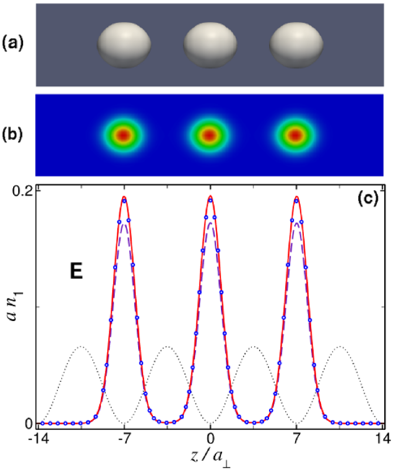
In terms of the underlying OL, this is the case of the tight-binding regime, . The nonlinear tight-binding regime is realized when the potential depth is much larger than both the linear and nonlinear (mean-field) energies (i.e.,). Under these circumstances, the condensate density is highly localized near potential minima, making the overlap between densities associated with different wells negligible. Point D in the first band gap of Fig. 1(c) corresponds to a fundamental GS with and . Since its peak axial density is , and implies , this fundamental GS belongs to the nonlinear tight-binding regime. Figure 4 shows a compound GS built of three such fundamental solitons. It corresponds to point E in Fig. 1(c). Its chemical potential, , is the same as that of the corresponding fundamental GS, and its number of particles, , now coincides with the sum of the number in its constituents (note that we always approximate to the nearest integer). As can be seen from Fig. 4, this compound soliton exhibits three well-separated identical peaks (BEC droplets), each one being practically indistinguishable from the above-mentioned fundamental GS. Figure 4(c) shows that the results obtained from the effective 1D equation (18) (the solid red line) agree very well with those produced by the full 3D GPE (17) (open circles). In particular, the 1D equation yields the particle number , which is very close to , as given by the 3D solution. Since represents a measurement of the norm of the wave function, it is clear that the error in the number of particles reflects the error in the corresponding wave functions. The 1D GPE (19), corresponding to the dashed blue line in Fig. 4(c), gives , which implies an error .
Point F in Fig. 1(c) corresponds to a fundamental GS located near the
top edge of the first band gap. This soliton, which is very similar to that
shown in Fig. 5, contains particles and has chemical potential
, which implies . At this
value of there is a significant probability of the excitation of higher
levels in the radial-confinement potential, which is corroborated by the fact
that the peak axial density of this GS is . Because
inequality does not hold in this case, one cannot expect the
ordinary 1D GPE (19) to be valid. In fact, it yields the number of
particles , which implies an error greater than . Nevertheless,
the effective nonpolynomial 1D equation (18) remains
valid and quite accurate. It produces , which corresponds to a
maximum error of . This is not surprising, since condition
(15), which guarantees the validity of the nonpolynomial equation, is
satisfied in this case.
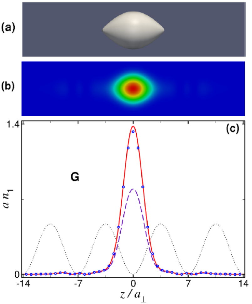
The solution pertaining to point G in Fig. 1(c) is qualitatively similar. It corresponds to the fundamental GS located near the top edge of the second band gap, with chemical potential and . Figure 5 shows the 3D density and axial linear density of this BEC droplet. In this case, , indicating a large contribution of excited radial modes. As a consequence, the ordinary 1D GPE (19) [the dashed blue line in Fig. 5(c)] fails to reproduce the 3D results (open circles). It predicts , which means the error exceeds . As seen from Fig. 5(c), the effective 1D equation (18) (the solid red line) remains accurate enough in this case, too. In particular, it yields , the respective error being .
The above results imply that, with the deep OL, the number of particles that can be accommodated in a fundamental GS can be large enough to make the 3D character of the wave function essential. In fact, even for the tight radial confinement (), which is the most favorable case for the applicability of the 1D approximation, the usual 1D GPE (19) with the deep OL potential cannot be reliably used beyond the first third of the first band gap. Since the validity of the mean field treatment requires , the usual GPE cannot be used close to the bottom edge of the band gap, either. It is thus clear that the range of validity of this standard 1D equation is limited. This conclusion becomes even more severe if one takes into account that the tight-radial-confinement regime is not easy to realize using typical experimental parameters. Our simulations indicate, however, that the effective nonpolynomial 1D equation (18) properly describes such essentially 3D situations, providing for an accurate description of the fundamental GSs in the entire band gaps.
III.2 Intermediate radial confinement:
This regime is of particular interest because it corresponds to typical experimental parameters. It can be realized, for instance, with a 87Rb condensate in an OL of period , radially confined by a harmonic potential with . The particle numbers of the GSs considered below are given for these physical parameters, and, they can be converted into values of for other situations by means of Eq. (22) (now, with ) .
Figure 6(a) shows the band-gap structure produced by the linearized version of Eq. (17) for zero-vorticity modes. Recall that the linearization of the effective 1D equations (18) and (19) yields, instead, the diagram displayed in Fig. 1(a) (except for the narrow band marked by the arrow, which, as already mentioned, does not appear in the 1D approximation). It is seen that the 1D approximation cannot reproduce the 3D picture resulting from the excitation of the radial modes, which manifest themselves in Fig. 6(a) as replicas of bands shifted up by integer multiples of . Since this quantity is smaller in the present case than it was before, the effect of these contributions in the region of interest is now stronger. While it is obvious that the 1D equations cannot account for the 3D effects originating from the shifted bands, we will demonstrate that these equations may still produce an accurate description of common GSs (i.e., those originating from the energy bands).
Figures 6(b) and 6(c) display the band-gap structure as a function of the quasimomentum for lattice depths and , respectively. Thin black lines in these figures represent 3D results that cannot be reproduced by the 1D models, and points H–M in plane mark examples of GSs that will be considered below.
III.2.1 Shallow optical lattice:
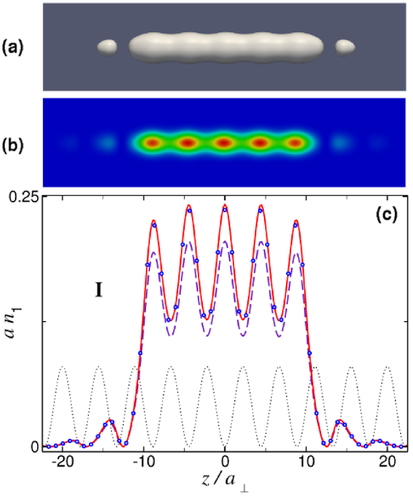
Point H in Fig. 6(b) corresponds to a fundamental GS with and , which is similar to the one in Fig. 3, but with the peak axial density . In this case, the effective 1D equation (18) predicts , thus corresponding to a error, while the 1D GPE (19) predicts (an error). Symmetric combinations of five such fundamental GSs generate the compound GS shown in Fig. 7, which contains particles and corresponds to point I in Fig. 6(b). The 3D density of this soliton exhibits five weakly separated peaks, as shown in Figs. 7(a) and 7(b) by means of the isosurface and the color map in the cross-section plane drawn through the axis. As seen in Fig. 7(c), in this case the effective 1D equation (18) yields an error of in the norm of the wave function () while the use the ordinary 1D GPE (19) generates an error of (), showing that, already for this GS, the 3D effects play an important role.
Point J in Fig. 6(b) corresponds to a fundamental GS containing particles and located near the top edge of the first band gap. It is qualitatively similar to the one shown in Fig. 3, but having and . In this case, Eqs. (18) and (19) yield results with an error () and (), respectively.
III.2.2 Deep optical lattice:
Points K, L, and M in Fig. 6(c) correspond to fundamental GSs in the case of the tight-binding underlying linear structure. The first soliton, which contains particles, with and axial density , also corresponds to the nonlinear tight-binding regime and is thus highly localized at a single lattice site. This follows from the fact that, for and , one has , which is much greater than the above-mentioned value of . For this GS, located near the bottom edge of the first band gap, the ordinary 1D GPE (19) yields an error , which continues to grow as one moves upward in the band gap. However, the effective nonpolynomial 1D equation (18) remains accurate within a deviation.
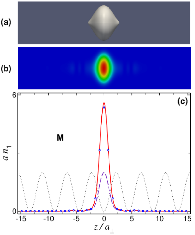
Point L in Fig. 6(c) indicates the position of a fundamental GS near the top edge of the first band gap, with , , and . Since the inequality does not hold in this case, the ordinary 1D GPE (19) is invalid, giving a error (). Note that, even though point L is relatively close to a 3D energy band [the thin black line in Fig. 6(c)], which cannot be reproduced by the effective 1D equation (18), it can, however, reproduce this GS within a error (). The same is true for the fundamental GS displayed in Fig. 8, which corresponds to point M in Fig. 6(c). It represents a BEC droplet containing particles, with and the peak axial density . Since we have in the present case, the system is no longer in the nonlinear tight-binding regime. This is seen in Fig. 8, where the density is not strongly localized around the minimum of the potential well. As seen in Fig. 8(c), the nonpolynomial 1D equation (18) yields results (the solid red line) that agree with the 3D picture produced by the full GPE (17) (open circles), within a deviation [Eq. (18) yields in this case]. On the contrary, the 1D GPE (19), which gives results (the dashed blue line) with an error (it yields ), clearly is not valid in this case.
These findings demonstrate that, in the physically relevant regime of the intermediate radial confinement (), even for the shallow OL the 3D effects may be important, and thus the usual 1D GPE (19) fails to reproduce correctly the axial density and the particle content . For and potential depth , the fundamental GSs located in the first band gap, as predicted by the 1D GPE equation, feature the error , which is still larger for compound GSs. For the deep OL (), the 1D GPE is valid only in a small region near the bottom edge of the first band gap. In general, this equation is applicable only where both conditions and hold simultaneously. As increases, the relative strength of the radial confinement decreases, and the range of validity of the 1D GPE becomes more and more narrow. From the experimental viewpoint, the increase of may be relevant because, in this way, one can easily increase the number of particles in the fundamental GSs. However, the increase of also implies a decrease in the relative size of the radial-excitation energy quantum, which can compromise the stability of the solitons because they can decay by exciting higher radial modes, even for condensates with a relatively small number of particles. We briefly consider this case below. The stability properties of the GSs will be analyzed in Sec. IV.
III.3 Weak radial confinement:
In this regime, the typical energy scale in the underlying linear problem is sufficiently large to easily excite higher transverse modes. As a representative example, we consider the case of , which can be realized in a 87Rb condensate in an OL with and radial-confinement strength . The particle contents of the GSs considered below correspond to such condensates. As before, the corresponding values of can be converted into those corresponding to other situations by means of Eq. (22) (this time, ).
Figure 9(a) displays the band-gap structure of the underlying 3D linear problem, to be compared with Fig. 1(a) which shows the band-gap structure obtained from the linearization of 1D equations (18) or (19). As before, the latter equations cannot account for the 3D contributions from the excited radial modes, which account for the series of shifted bands separated by gaps of value in Fig. 9(a). Figures 9(b) and 9(c) display the linear band-gap structure as a function of the quasimomentum for and , respectively.
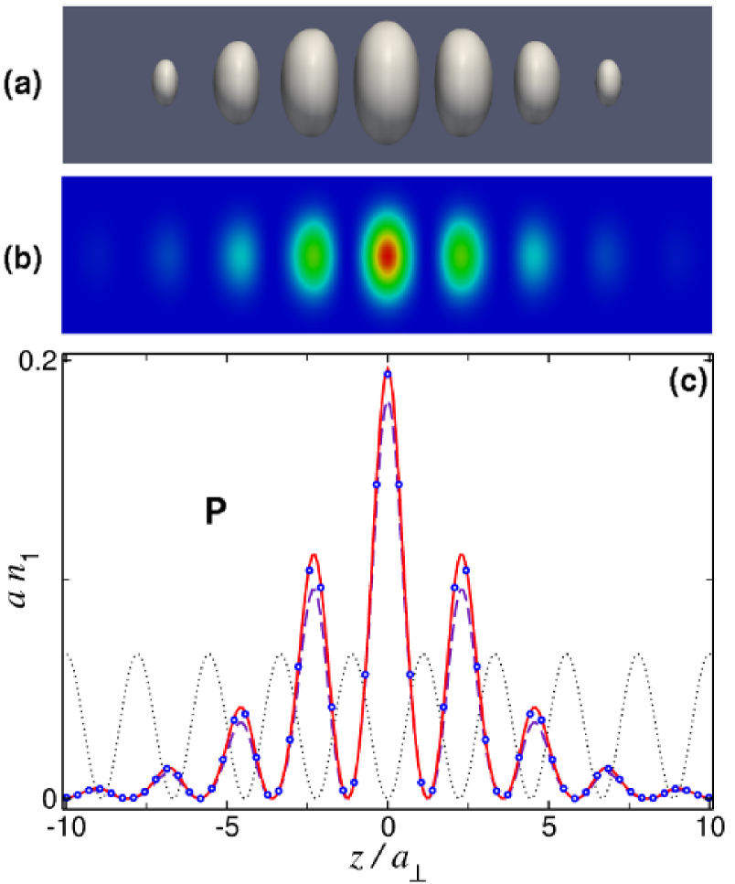
Point P in Fig. 9(b) corresponds to a fundamental GS with and . Its 3D density plot, shown in Fig. 10, demonstrates that this fundamental soliton is spread over several lattice sites, which is a consequence of the fact that its chemical potential is very close to the first linear energy band, where only extended solutions of the stationary GPE exist. Figure 10(c) shows that the results obtained from the effective 1D equation (18) (the solid red line) coincide with the 3D results (open circles) within (it predicts ). However, the 1D GPE (19) (the dashed blue line) gives rise to an error (it predicts ). We thus conclude that, in the weak-radial-confinement regime (), the latter equation is only applicable in a narrow region close to the bottom edge of the first band gap, even for shallow OLs. In this regime, the 3D contributions play an important role in most cases. These contributions are, however, well accounted for by the effective 1D equation (18). For instance, for point Q in Fig. 9(b) [which corresponds to a fundamental GS near the top edge of the first band gap, with , , and ] the 1D GPE (19) gives an error of (), while the nonpolynomial 1D equation (18) limits the error to (). Point R in Fig. 9(c) is an example of a fundamental GS in a deep OL. It corresponds to a disk-shaped BEC droplet trapped in a single lattice cell [see Fig. 11(b)], which contains 87Rb atoms, and has . Its axial linear density is qualitatively similar to that shown in Fig. 8(c), but with a maximum value . In this case, the 1D GPE predicts the particle content , while the effective 1D equation (18) yields , which corresponds to an error in the norm of the wave function. Thus, the 1D nonpolynomial equation provides for a sufficiently good description of the stationary GSs even in the highly nonlinear () weak-radial-confinement regime.
IV STABILITY ANALYSIS
We have investigated the stability of the GS solutions by monitoring their long-time behavior after the application of a random perturbation Wu2 ; JYang . Specifically, we have perturbed the corresponding wave functions with a small-amplitude () additive Gaussian white noise and have monitored the subsequent nonlinear evolution for . To this end we have numerically solved the full 3D GPE (1), as well as the effective 1D equation (14), using a Laguerre-Fourier pseudospectral method with a third-order Adams-Bashforth time-marching scheme. Numerical integration of the 3D GPE for such a long time is a very demanding computational task. While it is possible for a certain GS to be metastable and decay on a time scale still longer than , in practice this time is long enough in comparison with the lifetime of the condensate per se, hence the soliton surviving for may be categorized as stable.
We have found that both the full 3D GPE (1) and the effective nonpolynomial 1D equation (14) lead to the same conclusions regarding the stability of the GSs. However, once an unstable soliton begins to decay, one cannot expect, in general, the latter equation to reproduce the dynamical behavior correctly. The reason for this problem is that, as already mentioned in Sec. II, in the presence of the OL potential the above-mentioned adiabatic condition (i) is hard to fulfill in time-dependent settings. Of course, the same is true for the 1D equation (3), which is a limit form of Eq. (14) and, consequently, has a much narrower range of applicability. The results presented below have been obtained using the full 3D GPE (1). For each GS we have used at least two different basis sets and time steps to check that the results do not depend on details of the numerical procedure.
Our simulations demonstrate that, in general, fundamental GSs are stable, except in a narrow region close to the top edge of the band gaps. In particular, the solitons corresponding to points A, D, K, and P in Figs. 1, 6, and 9 remain stable up to . On the contrary, GSs in a shallow OL (), located close to the top edge of a band gap, such as those corresponding to points C, H, J, and Q in Figs. 1, 6, and 9, turn out to be unstable. This instability manifests itself as a steady decay of the norm of the GS through emission of radiation, on a time scale that increases as one moves away from the top edge of the band gap. In this regard, one finds that the GS corresponding to point H decays much slower than the other ones. As the lattice depth increases, in general, GSs become more stable and the instability region shrinks. In particular, our simulations indicate that GSs such as those corresponding to points F, G, L, M and R in Figs. 1, 6, and 9 (which are fundamental GSs in the deep OL, with , located close to the top edge of the band gap) also remain stable up to . This is in good agreement with previous analyses carried out in the context of deep optical lattices in terms of the ordinary 1D GPE (3) Kiv1 ; Wu2 .

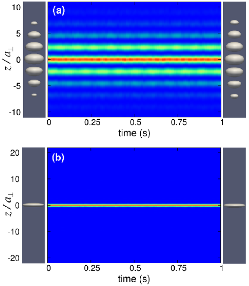
An important result is that fundamental GSs remain stable even in the weak-radial-confinement regime (). In this regime, GSs always have sufficient energy to excite higher radial modes, and, as a consequence, the 3D effects are always relevant and the usual 1D GPE (3) fails. Figure 11(a) displays the long-time behavior, after the application of the perturbation, of the fundamental GS shown in Fig. 10 [it corresponds to point P in Fig. 9(b)]. This figure shows (by means of a color map) the evolution of the axial density , which has been obtained from the 3D wave function by integrating out the radial dependence, as per Eq. (5). The left panel in this figure shows the 3D condensate density at (i.e., just after the application of the perturbation) as an isosurface taken at of the maximum density, while the right panel represents the density at . This GS has , which implies . Note that, despite the fact that this chemical potential is greater than the quantum , the GS remains stable up to . The same is true for the fundamental GS corresponding to point R in Fig. 9(c), which corresponds to a disk-shaped BEC containing more than 87Rb atoms with chemical potential . As Fig. 11(b) shows, this GS also remains stable.
Our simulations also demonstrate that the compound GS from Fig. 2, corresponding to point B in Fig. 1(b), is unstable. This is seen in Fig. 12(a), which shows how the soliton decays on a time scale after the addition of a white-noise perturbation. This compound GS, which has and , was built in the shallow OL () as the symmetric combination of three fundamental constituents. We have found that, in such shallow lattices, GSs of this type are always unstable. However, it is not difficult to find stable solitons of this type in somewhat deeper lattices. An example is shown in Fig. 12(b), which represents a stable three-peak soliton with and , trapped in the OL with and . Similar dynamics is observed for the GS displayed in Fig. 7, which corresponds to point I in Fig. 6(b). This is a five-peak compound generated in the shallow OL () in the regime of the intermediate radial-confinement strength (). Our simulations indicate that this compound soliton is unstable. In fact, no stable five-peak solitons were found in such a shallow lattice. On the other hand, it is not difficult to find stable compounds of this kind for deeper OLs. An example is the five-peak pattern with , , , and . In general, GSs naturally become more stable as the lattice depth increases. For deep OLs (), the stability of compound GSs is essentially identical to that of their fundamental constituents. The GS in Fig. 4, which corresponds to point E in Fig. 1(c), is an example of a stable three-peak soliton realized in a deep OL.
V CONCLUSIONS
To appraise the physical relevance of the results reported in this work, it is pertinent to recall that the mean-field treatment of the GSs (gap solitons), based on the GPE, is valid if and the condensate is sufficiently dilute so that , where is the scattering length of the inter-atomic collisions and is the atomic density. In shallow OLs (optical lattices) such conditions can be easily met, though the former one imposes a serious limitation on the range of applicability of the usual 1D GPE (19), which fails as increases. In deep OLs, where the tunneling between adjacent cells is strongly suppressed, the above conditions must be fulfilled at each site of the lattice. Under these circumstances, GSs may have a rather high local density. A good estimate for the 3D peak density in terms of the peak axial density, , can be obtained from the following relation PRA77 :
| (25) |
Substituting the values of obtained in Section III for different GSs into Eq. (25), one can easily verify that condition is satisfied in all cases, which justifies the use of the mean-field description. The most critical situation occurs for the GS corresponding to point G in Fig. 1(c), which has . For the GS corresponding to point R in Fig. 9(c), one finds .
Despite the fact that applicability conditions for the mean-field treatment can be readily met, it is much harder to justify the validity of the usual 1D GPE (3), which requires both conditions and to hold simultaneously. Only in this case may the 3D effects be safety neglected. In most experimentally relevant situations, these conditions are not met, hence the applicability range of Eq. (3) turns out to be very limited. On the contrary, it has been shown in this work that the effective 1D GPE (14) with the nonpolynomial nonlinearity provides for an accurate description of the stationary matter-wave GSs in most cases of practical interest.
A relevant extension of the present analysis may be to GSs with intrinsic vorticity, as well as to mobility of stable solitons. It is also interesting to consider two-component GSs in the realistic 3D setting.
Acknowledgements.
V.D. acknowledges financial support from Ministerio de Ciencia e Innovación through contract No. FIS2009-07890 (Spain).References
- (1) V. A. Brazhnyi and V. V. Konotop, Mod. Phys. Lett. B 18, 627 (2004).
- (2) O. Morsch and M. Oberthaler, Rev. Mod. Phys. 78, 179 (2006).
- (3) R. Carretero-González, D. J. Frantzeskakis, and P. G. Kevrekidis, Nonlinearity 21, R139 (2008).
- (4) Emergent Nonlinear Phenomena in Bose-Einstein Condensates: Theory and Experiment, edited by P. G. Kevrekidis, D. J. Frantzeskakis, and R. Carretero-González (Springer, Heidelberg, Germany, 2007).
- (5) Y. V. Kartashov, B. A. Malomed, and L. Torner, Rev. Mod. Phys. 83, 247 (2011).
- (6) E. P. Gross, Nuovo Cimento 20, 454 (1961); J. Math. Phys. 4, 195 (1963); L. P. Pitaevskii, Zh. Eksp. Teor. Fiz. 40, 646 (1961) [Sov. Phys. JETP 13, 451 (1961)].
- (7) A. Muñoz Mateo and V. Delgado, Phys. Rev. Lett. 97, 180409 (2006).
- (8) J. A. M. Huhtamäki, M. Möttönen, T. Isoshima, V. Pietilä, and S. M. M. Virtanen, Phys. Rev. Lett. 97, 110406 (2006).
- (9) P. J. Y. Louis, E. A. Ostrovskaya, C. M. Savage, and Y. S. Kivshar, Phys. Rev. A 67, 013602 (2003).
- (10) F. Kh. Abdullaev and M. Salerno, Phys. Rev. A 72, 033617 (2005).
- (11) T. Mayteevarunyoo and B. A. Malomed, Phys. Rev. A 74, 033616 (2006).
- (12) Y. Zhang and B. Wu, Phys. Rev. Lett. 102, 093905 (2009).
- (13) Y. Zhang, Z. Liang, and B. Wu, Phys. Rev. A 80, 063815 (2009).
- (14) A. Muñoz Mateo, V. Delgado, and B. A. Malomed, Phys. Rev. A 82, 053606 (2010).
- (15) A. E. Muryshev, G. V. Shlyapnikov, W. Ertmer, K. Sengstock, and M. Lewenstein, Phys. Rev. Lett. 89, 110401 (2002).
- (16) L. Salasnich, A. Parola, and L. Reatto, Phys. Rev. A 65, 043614 (2002); L. Salasnich, Laser Phys. 12, 198 (2002).
- (17) A. Muñoz Mateo and V. Delgado, Phys. Rev. A 77, 013617 (2008); 75, 063610 (2007); Ann. Phys. (NY) 324, 709 (2009).
- (18) S. Middelkamp, G. Theocharis, P. G. Kevrekidis, D. J. Frantzeskakis, and P. Schmelcher, Phys. Rev. A 81, 053618 (2010).
- (19) G. Theocharis, A. Weller, J. P. Ronzheimer, C. Gross, M. K. Oberthaler, P. G. Kevrekidis, and D. J. Frantzeskakis, Phys. Rev. A 81, 063604 (2010).
- (20) C. Wang, P. G. Kevrekidis, T. P. Horikis, D. J. Frantzeskakis, Phys. Lett. A, 374, 3863 (2010).
- (21) S. Middelkamp, J. J. Chang, C. Hamner, R. Carretero-González, P. G. Kevrekidis, V. Achilleos, D. J. Frantzeskakis, P. Schmelcher, and P. Engels, Phys. Lett. A 375, 642 (2011).
- (22) An independent derivation of this formula was reported by F. Gerbier, Europhys. Lett. 66, 771 (2004).
- (23) L. Salasnich, B.A. Malomed, and F. Toigo, Phys. Rev. A 76, 063614 (2007).
- (24) A. Muñoz Mateo and V. Delgado, Phys. Rev. A 74, 065602 (2006).
- (25) S. Adhikari and B.A. Malomed, Europhys. Lett. 79, 50003 (2007); Physica D 238, 1402 (2009).
- (26) F. H. Mies, E. Tiesinga, and P. S. Julienne, Phys. Rev. A 61, 022721 (2000).
- (27) B. Eiermann, Th. Anker, M. Albiez, M. Taglieber, P. Treutlein, K.-P. Marzlin, and M. K. Oberthaler, Phys. Rev. Lett. 92, 230401 (2004).
- (28) J. Armijo, T. Jacqmin, K. Kheruntsyan, and I. Bouchoule, Phys. Rev. A 83, 021605(R) (2011).
- (29) J. Yang and Z. H. Musslimani, Opt. Lett. 28, 2094 (2003).