Gated Recurrent Unit (GRU) for Emotion Classification from Noisy Speech

Rajib Rana1, Julien Epps2, Raja Jurdak3, Xue Li4, Roland Goecke5, Margot Brereton6 and Jeffrey Soar7 1Institute of Resilient Regions (IRR)
University of Southern Queensland, Springfield, QLD 4300
Email: rajib.rana@usq.edu.au 2School of Electrical Engineering and Telecommunications, University of New South Wales
3Distributed Sensing Systems, CSIRO-Data61 4School of Information Technology and Electrical Engineering, University of Queensland
5Information Technology & Engineering, University of Canberra
6Computer Human Interaction, Queensland University of Technology
7School of Management and Enterprise, University of Southern Queensland

Abstract

Despite the enormous interest in emotion classification from speech, the impact of noise on emotion classification is not well understood. This is important because, due to the tremendous advancement of the smartphone technology, it can be a powerful medium for speech emotion recognition in the outside laboratory natural environment, which is likely to incorporate background noise in the speech. We capitalize on the current breakthrough of Recurrent Neural Network (RNN) and seek to investigate its performance for emotion classification from noisy speech. We particularly focus on the recently proposed Gated Recurrent Unit (GRU), which is yet to be explored for emotion recognition from speech. Experiments conducted with speech compounded with eight different types of noises reveal that GRU incurs an 18.16% smaller run-time while performing quite comparably to the Long Short-Term Memory (LSTM), which is the most popular Recurrent Neural Network proposed to date. This result is promising for any embedded platform in general and will initiate further studies to utilize GRU to its full potential for emotion recognition on smartphones.

I Introduction

Automatic Speech Emotion Recognition has gained increasing interest in both research and commercial space due to its tremendous potential to determine affective states [1]. Automatic Speech emotion recognition can offer unprecedented opportunities for the Human-Computer Interaction Systems, as for example, recommendation systems can be designed to make more accurate affect-sensitive recommendations [2]. This will also be highly beneficial for the burgeoning health and wellbeing applications as, for example, affect-diaries can be built to keep people aware of any prolonged negative mood, which would potentially prevent the onset or relapse of affective disorders [3].

In recent years, Deep Learning models have revolutionized many fields, in particular, automatic speech recognition and computer vision [4, 5]. These models have also achieved improved performance in emotion recognition compared to conventional machine learning algorithms. For example, [6, 7, 8, 9, 10, 11, 12], and [13] present some best reported results for affective speech analysis using deep learning models.

Out of the many forms of Deep Learning models, we consider Recurrent Neural Networks (RNNs) as they are targeted to model the long range dependencies between successive observations. Speech emotion possesses temporal dependency as it is unlikely to change rapidly between subsequent speech utterances [14]. Therefore, the Recurrent Neural Networks are most suitable for emotion recognition from speech. However, RNNs often suffer from the classical “Vanishing” and “Exploding” Gradient problems, which results in failing to learn long-range dependencies. To avoid this, two variants of Recurrent Neural Networks have been proposed, which uses a “gating” approach to avoid these problems: (1) Long Short-Term Memory (1997) [15] and (2) Gated Recurrent Unit (2014) [16].

Smartphones are great platforms for speech emotion recognition, as people are close to their phones for an extended period of time. Research shows that almost 79% of people have their smartphones with them 22 hours a day¹¹1http://www.adweek.com/socialtimes/smartphones/480485. In addition, the processing capacity of the modern smartphones is also extraordinary. In the scope of this paper we assume that speech samples are collected during phone conversation [17].

The key challenge of emotion recognition from phone conversation is background noise as people can talk over phone anywhere including the cafeteria, park, office and many more places. The mainstream research in emotion recognition from speech has mainly focused on clean speech captured in controlled laboratory environment. Therefore, the impact of noise in emotion classification is not well understood [18].

Another major hurdle of running any Deep Learning models on a smartphone is computational complexity. Despite the advancement in the processing capacity, smartphones are still limited by battery power. Therefore, a method with a small runtime is a must. Amongst LSTM and GRU, GRU has relatively simplified architecture, therefore, our focus is mainly on GRU. A number of studies have looked into the performance of LSTM (e.g., [19, 20, 21]) for emotion recognition from speech, however, the performance of GRU for that is currently unexplored.

In this paper, we address the above two challenges. The contributions of this paper are as follows:

1.

To the best of our knowledge we for the first time analyze the accuracy and the run-time complexity of Gated Recurrent Unit for emotion classification from speech.
2.

We superimpose various real-life noises on clean speech and analyze the classification performance of the Gated Recurrent Unit under various noise exposures.
3.

We use LSTM as the benchmark and conduct a detailed accuracy and run-time comparisons of these two gating Recurrent units for emotion classification from noisy speech.

The paper is organized as follows. In next section, we provide background information on Recurrent Neural Networks followed by the description of how GRU can be used for emotion classification from a noisy speech in Section III. We then present the results, and discussion in Section IV. This is followed by existing work in Section V; and finally, we conclude in Section VI.

Refer to caption — Figure 1: Recurrent Neural Networks.

II Recurrent Neural Networks

The conventional Feed Forward Neural Network is trained on labeled data until it minimizes the prediction error. Whereas the decision an RNN reached at time step $t-1$ affects the decision it will reach at time step $t$ . Therefore, RNNs have two input sources: the present, and the recent past, which it uses in combination in determining a response to a new input.

An example Recurrent Neural Networks (RNNs) is shown in Figure 1 and the related symbols are defined in Table I. A hidden state ( $s_{t}$ ) is a non-linear transformation of a linear combination of input ( $x_{t}$ ) and previous hidden state ( $s_{t-1}$ ). Output ( $o_{t}$ ) at time $t$ is only dependent on the current hidden state $s_{t}$ . The output is associated with a probability $p_{t}$ determined through a “softmax” function. In Neural Networks a softmax function is implemented in the final layer of a network used for classification. For a classification with $K$ classes, the softmax function determines the probability of a probe being classified as each of the $K$ classes.

	$\displaystyle s_{t}$	$\displaystyle=$	$\displaystyle tanh(Ws_{t-1}+Ux_{t})$
	$\displaystyle o_{t}$	$\displaystyle=$	$\displaystyle Vs_{t}$

TABLE I: Symbol Definitions

Symbol	Definition
$x_{t}\in\mathbb{R}^{d}$	$d$ dimensional input vectors
$S_{t}\in\mathbb{R}^{p}$	$p$ dimensional hidden unit
$O_{t}\in\mathbb{R}^{d^{\prime}}$	$d^{\prime}$ dimensional outputs
$U\in\mathbb{R}^{d\times p}$	maps $d$ -dimensional input to $p$ dimensional hidden unit
$V\in\mathbb{R}^{p\times d^{\prime}}$	maps $p$ dimensional hidden unit to $d^{\prime}$ dimensional output
$W\in\mathbb{R}^{p\times p}$	maps $p$ dimensional hidden unit to another hidden unit.

Vanishing and Exploding Gradients: Both of these terms were introduced by Bengio et al. [22] in 1994. The exploding gradient problem refers to the large increase in the norm of the gradient during training. The vanishing gradient problem refers to the opposite behavior when long-term components go exponentially fast to norm 0, making it impossible for the model to learn the correlation between temporally distant events.

Any quantity multiplied frequently by an amount slightly greater than one can become immeasurably large (exploding). Multiplying by a quantity less than one is also true (vanishing). Because the layers and time steps of deep neural networks relate to each other through multiplication, derivatives are susceptible to vanishing or exploding.

Encouragingly, there are a few ways to address these gradient problems. Proper initialization of the weight (W) matrix and regularization can reduce the impact of vanishing gradients. Another possible solution is to use the Rectified Linear Unit (ReLU) [23] instead of the conventional $tanh$ or sigmoid activation functions. The ReLU derivative is either $0$ or $1$ , so it is not as likely to cause a vanishing or exploding gradient. However, ReLU units can be fragile during training and can “die”. For example, a large gradient flowing through a ReLU neuron could cause the weights to update in such a way that the neuron will never activate on any data point again. As a result as much as 40% of the neurons will never be activated across the entire training dataset if the learning rate is set too high. With a rigorously chosen learning rate, this can be avoided.

An even more effective solution is to use the gated Recurrent Neural Network architectures: Long Short-Term Memory (LSTM) or Gated Recurrent Unit (GRU). LSTMs first proposed by Hochreiter et al. in 1997 are one of the most widely used Recurrent Neural Networks today. GRUs, first proposed in 2014, are simplified versions of LSTMs. Both of these RNN architectures were purposely built to address the vanishing and the exploding gradient problem and efficiently learn long-range dependencies. To assist the understanding of GRU in the next section we first describe LSTM.

II-A Long Short-Term Memory Units (LSTMs)

The Long Short Term memory is a special kind of Recurrent Neural Networks, that eliminates the shortcoming of vanishing or exploding gradient problem of the Recurrent Neural Networks. This makes LSTM suitable to learn from history to classify, process and predict time series when there are very long and unknown time lags between important events. An LSTM network is made up of LSTM blocks that have three gates: input, output and forget gate, which help it to remember a value for an arbitrary long time; forget the value when it is not important to remember anymore or output the value. LSTMs help preserve the error that can be backpropagated through time and layers. By maintaining a more constant error, they allow recurrent nets to continue to learn over many time steps, for example over 1000.

LSTMs contain information outside the normal flow of the recurrent network in a gated cell. Information can be stored in, written to, or read from a cell, much like data in a computer’s memory. The cell makes decisions about what to store, and when to allow reads, writes, and erasures, via gates that open and close. Unlike the digital storage on computers, however, these gates are analog, implemented with element-wise multiplication by sigmoids, which are all in the range of $[0-1]$ . Analog has the advantage over digital of being differentiable, and therefore suitable for backpropagation.

Those gates act on the signals they receive, and similar to the neural network’s nodes, they block or pass on information based on its strength and import, which they filter with their own sets of weights. Those weights, like the weights that modulate input and hidden states, are adjusted via the recurrent networks learning process. That is, the cells learn when to allow data to enter, leave or be deleted through the iterative process of making predictions, backpropagating error, and adjusting weights via gradient descent.

LSTMs’ memory cells give different roles to addition and multiplication in the transformation of input. Instead of determining the subsequent cell state by multiplying its current state with new input, they add the two, which helps them preserve a constant error when it must be backpropagated at depth.

Different sets of weights filter the input for input, output, and forgetting. The forget gate is represented as a linear identity function, because if the gate is open, the current state of the memory cell is simply multiplied by one, to propagate forward one more time step.

The LSTMs need a forget gate although their purpose is to link distant occurrences to a final output. This can be justified with an example. While analyzing a text corpus when the pointer comes to the end of a document, it could be the case the next document does not have a correlation with the previous one. Therefore, the memory cell should be set to zero before the net ingests the first element of the next document.

An LSTM cell has been shown in Fig 2(a). It is not limited to computing the weighted sum of the inputs and then appliying a nonlinear function; rather each $j$ -th LSTM unit maintains a memory $c_{t}^{j}$ at time $t$ . The activation function of the LSTM is

\displaystyle h_{t}^{j}=o_{t}^{j}\tanh{c_{t}^{j}}.

The output gate $o_{t}^{j}$ modulates the amount of memory content exposure. With $V_{o}$ as a diagonal matrix, It is calculated by

\displaystyle o_{t}^{j}=\sigma(W_{o}x_{t}+U_{f}h_{t-1}+V_{o}c_{t})^{j}.

The memory $c_{t}^{j}$ is updated by partially forgetting the existing memory and adding a new memory $\tilde{c}_{t}^{j}$ . The extent to which the existing memory is forgotten is controlled by a forget gate $f_{t}^{j}$ .

\displaystyle f_{t}^{j}=\sigma(W_{f}x_{t}+U_{o}h_{t-1}+V_{i}c_{t-1})^{j}.

And the extent to which new memory is added is controlled by an input gate $i_{t}^{j}$

\displaystyle i_{t}^{j}=\sigma(W_{i}x_{t}+U_{i}h_{t-1}+V_{f}c_{t-1})^{j}.

Controlled by these gates the existing memory is updated using the following equations.

	$\displaystyle\tilde{c}_{t}^{j}$	$\displaystyle=$	$\displaystyle\tanh{(W_{c}x_{t}+U_{c}h_{t-1})^{j}},$
	$\displaystyle{c}_{t}^{j}$	$\displaystyle=$	$\displaystyle f_{t}^{j}c_{t-1}^{j}+i_{t}^{j}\tilde{c}_{t}^{j}.$

TABLE II: LSTM vs GRU

	LSTM	GRU
Controlled Memory Exposure	The amount of memory seen by the other	The whole memory is exposed to the network
	units of the network is controlled by the Output Gate
New Memory Computation	No separate control for amount of	Controls the information flow from the previous activation
	information flow from the previous time step
Complexity vs Performance	With an additional gate	Has fewer parameters and
	is likely to have higher complexity	thus may train comparatively faster or need less data to generalize

II-B Gated Recurrent Units (GRUs)

The Gated Recurrent Unit is a slightly more simplified variation of the LSTM. It combines the forget and input gates into a single “update gate” and has an additional “reset gate”. The end model is simpler than standard LSTM models and is becoming increasingly popular.

A Gated Recurrent Unit like LSTM modulates information inside the unit, however, without having a separate memory cell (see Fig 2(b)). The activation $h_{t}^{j}$ of the GRU at time $t$ is a linear interpolation between the previous activation $h_{t-1}^{j}$ and the candidate activation $\tilde{h}_{t}^{j}:$

\displaystyle h_{t}^{j}=(1-z_{t}^{j})h_{t-1}^{j}+z_{t}^{j}\tilde{h}_{t}^{j}

The update gate $z_{t}^{j}$ decides how much the unit updates its activation.

\displaystyle z_{t}^{j}=\sigma(W_{z}x_{t}+U_{z}h_{t-1})^{j}.

The candidate activation $\tilde{h}_{t}^{j}$ is computed similarly to the update gate:

\displaystyle\tilde{h}_{t}^{j}=tanh(Wx_{t}+U(r_{t}.*h_{t-1}))^{j},

[15] where $r_{t}^{j}$ is a set of reset gates and $.*$ denotes an element-wise multiplication. When the reset gate is off ( $r_{t}^{j}==0$ ), it allows the unit to forget the past. This is analogous to letting the unit reading the first symbol of an input sequence. The reset gate is computed using the following formula

\displaystyle r_{t}^{j}=\sigma(W_{r}x_{t}+_{r}h_{t-1})^{j}

Update gate $z$ controls how much the past state should matter now. Units with short-term dependencies will have active reset gates $r$ . Units with long-term dependencies have active update gates $z$ .

GRU and LSTM have many commonalities, yet there are some differences between these two, which we summarize in Table II.

III Gated Recurrent Unit for Emotion Classification from Noisy Speech

An emotion classification framework embodying a Gated Recurrent Unit is shown in Fig. 3. Our focus is on emotion classification from noisy speech, so we simulate noisy speech upon superimposing various environmental noises on clean speech. Features are extracted from the noisy speech and feed to the GRU for emotion classification. We have used the same framework for LSTM to contrast its classification performance with that of GRU.

III-A Description of Datasets

The Berlin emotional speech database [burkhardt2005database] is used in experiments for classifying discrete emotions. In this database, ten actors, five males and five females each uttered ten sentences (5 short and 5 longer, typically between 1.5 and 4 seconds) in German to simulate seven different emotions: anger, boredom, disgust, anxiety/fear, happiness, and sadness. Utterances scoring higher than 80% emotion recognition rate in a subjective listening test are included in the database. We classify all the seven emotions in this work. The numbers of speech files for these emotion categories in the presented Berlin database are: anger (127), boredom (81), disgust (46), fear (69), joy (71), neutral (79) and sadness (62). We use this prototypical database for the preliminary investigation of GRU’s performance for emotion recognition.

In order to simulate noise-corrupted speech signals, the DEMAND (Diverse Environments Multi-channel Acoustic Noise Database) noise database [thiemann2013diverse] has been used in this paper. This database involves 18 types of noises wherein we have used noise from traffic, cafe, living room, park, washing, car, office and river. The recordings were captured at a sampling rate of 48 kHz and with a target length of 5 minutes (300 s). Actual audio capture time was slightly longer thereby allowing the removal of set-up noises and other artifacts by trimming. The recorded signals were not subject to any gain normalization. Therefore, the original noise power in each environment was preserved.

III-B GRU Implementation

We use the PyBrain Toolbox [24] to implement the GRU. We evaluate the classification performance across three parameters including learning rate, number of cells and bias. To use GRU and LSTM for classification we use softmax function in the output layer. The Pybrain package uses $75\%$ of data for training and $25\%$ for validation. For accuracy we use the validation error in the plots.

III-C Feature Selection

For each speech segment, we choose a 13 coefficient Mel Frequency Cepstral Coefficients (MFCC) as a feature vector, which have been used by many researchers (e.g., [25],[25] and many more.) for emotion classification from speech. We choose the small number of coefficients for dimensionality reduction of feature space. Large feature sets consume a significant amount of memory, jointly with computing and power resources and they do not always contribute to improving the recognition rate.

IV Results and Discussions

IV-A Bias and Learning Rate

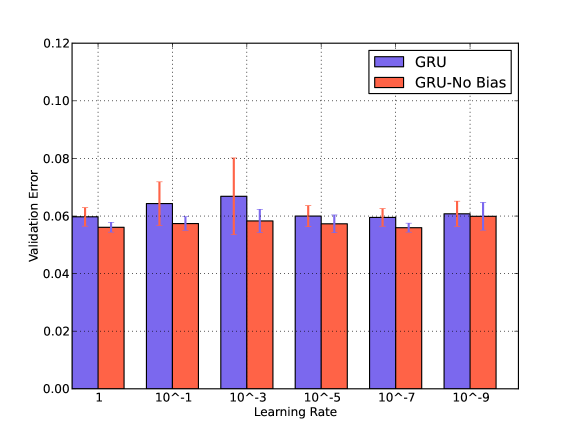
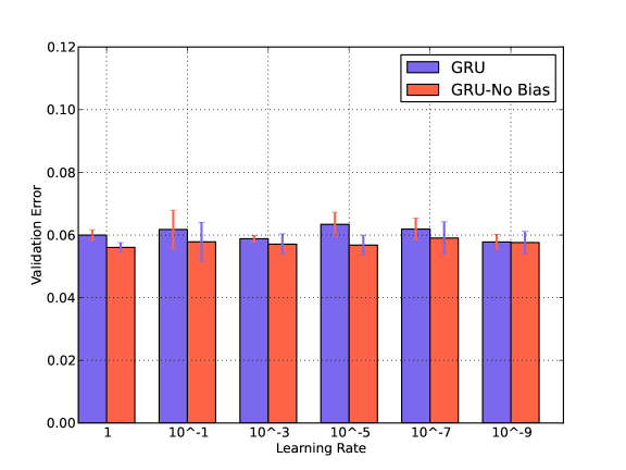
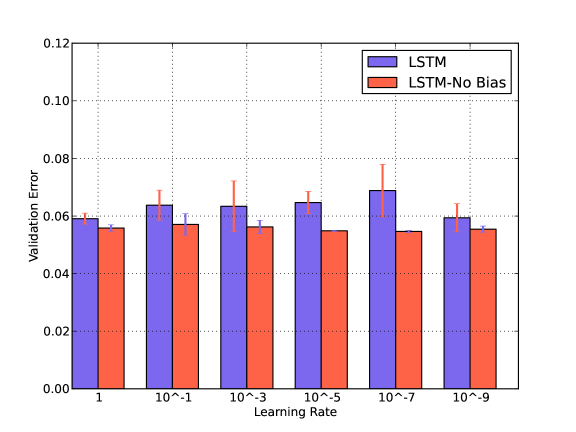
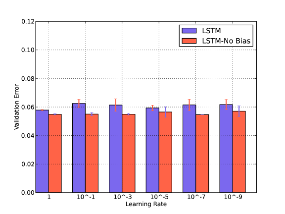
We compare the classification performance of GRU with respect to Bias and Learning Rate in Fig. 4. We reduce the learning rate gradually from 1 to $10^{-}9$ in the presence and absence of the bias. We find that learning rate has a very small impact and GRU performs better without the bias terms. Similar performances have been observed for LSTM. These behaviors can be observed in the noisy conditions as well. We have shown results for arbitrarily chosen Traffic noise.

Setting learning rates for plain Stochastic Gradient Descent in a neural network is usually a process of starting with an initial arbitrary value such as $0.01$ and then doing a cross-validation to find an optimal value. Common values range over a few orders of magnitude from $0.0001$ up to $1$ . A small value is desired to avoid overshooting, but a very small value cannot be chosen to avoid getting stuck in local minima or taking long to descend. For our experiments, a learning rate of $1$ yields the best performance.

Again a Bias value usually allows to shift the activation function to the left or right, which might be necessary for successful learning. However, in our case adding a bias has a negative impact, it lowers the accuracy.

IV-B Bias and Number of Cells

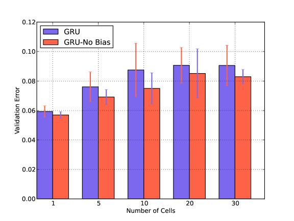
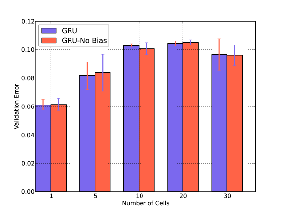
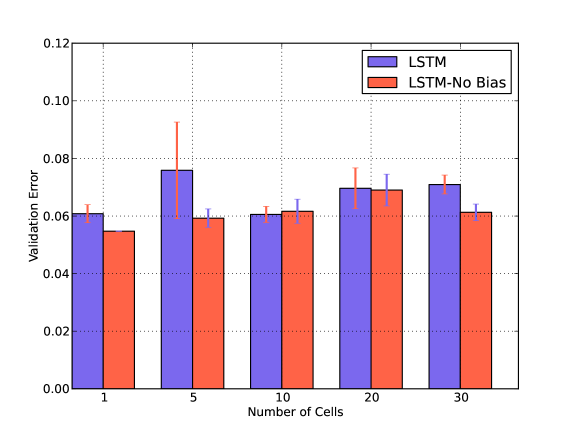
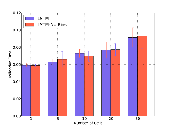
We also verify the impact of Number of Cells in presence and absence of Bias in Fig. 5. For both GRU and LSTM, the error is minimum when the number of cells is one and there is no bias term. Similar behavior is observed in presence of noise. We have shown the results for an arbitrary chosen Washing noise.

Both GRU and LSTM layers consist of blocks which in turn consist of cells. We anticipate that due to the smaller size of our dataset the increase in the number of cells does not have a positive impact

IV-C Accuracy: GRU versus LSTM

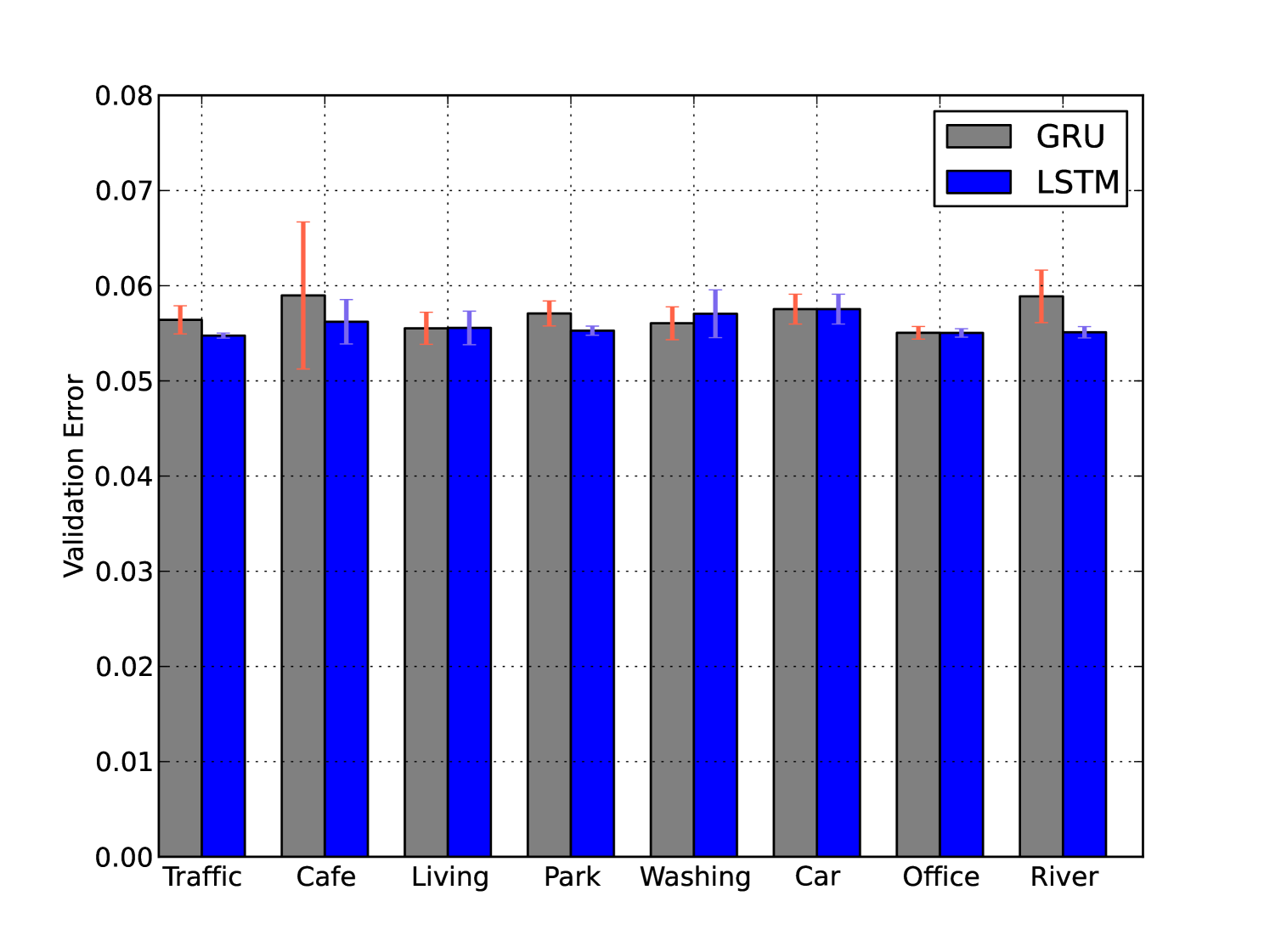
After analyzing the values of Number of Cells and Learning Rate and Bias, we now compare the performance of GRU and LSTM in various noisy conditions in Fig. 6. In the following, we use the following values for the three parameters: Number of cell = $1$ , Bias = False, Learning Rate = $1$ .

Out of eight different noise cases, in three cases LSTM and GRU performs the same (see Fig. 6(a)). While imputed with the Washing noise, GRU performs better than LSTM by $1.75\%$ . For four remaining noise imputations LSTM performs better than GRU. Amongst these, for Cafe and River noise LSTM performs noticeably ( $4.6\%$ and $6.4\%$ , respectively) better than GRU, but for Traffic and Park noise, it only performs marginally better than GRU.

The comparison results between LSTM and GRU provide some intuitive insights. For example, GRU performs better for the Washing noise which can be very periodic and not usually continuous. Whereas, LSTM performs noticeably better than GRU in the case of River and Cafe, which are usually sources of continuous noise. We will conduct further studies in future to explain the differences between GRU and LSTM.

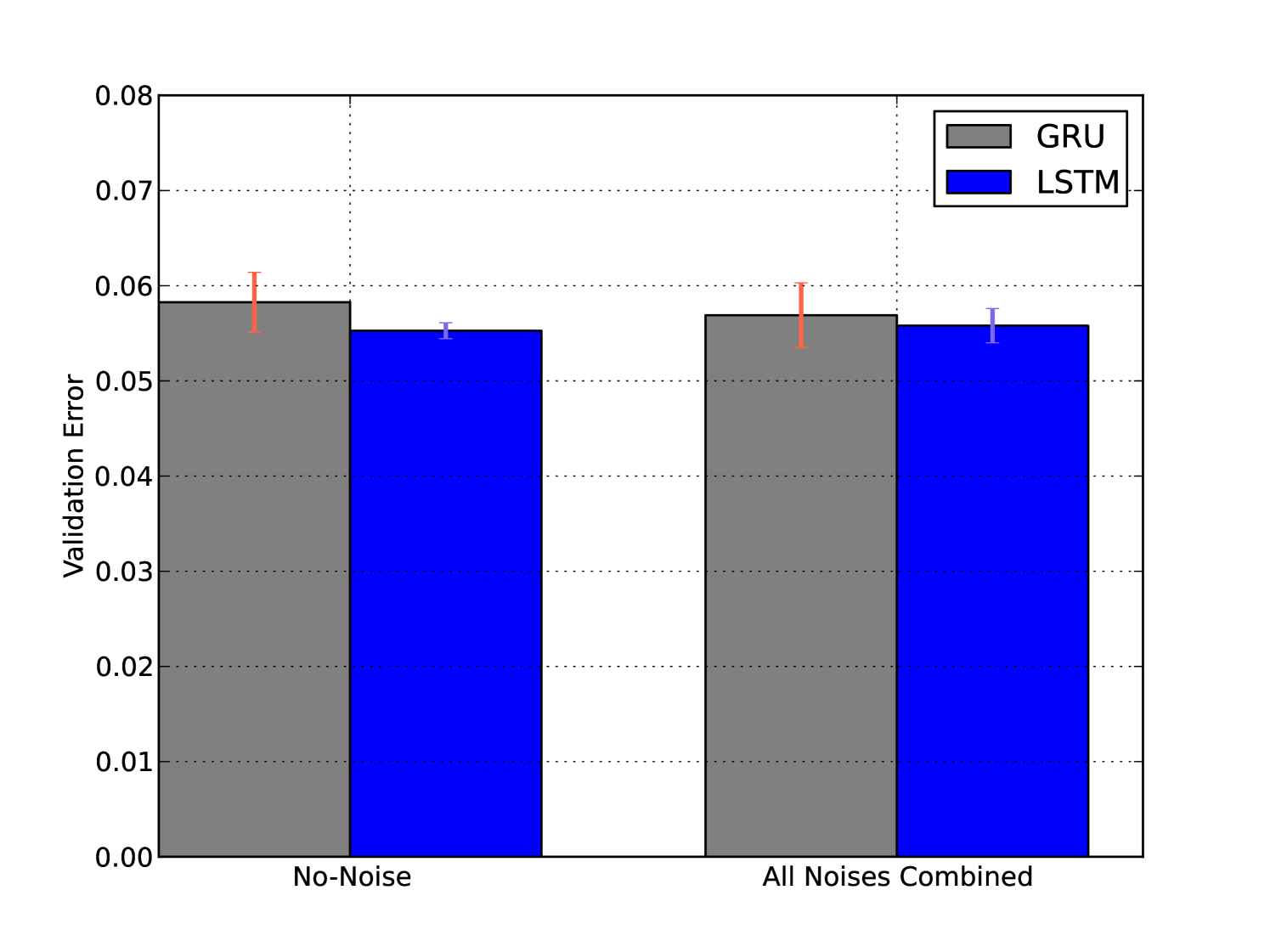
Using Fig. 6(b) we can understand the impact of noise (as a whole) on GRU’s performance where we compare the error at no-noise with the error combined at all other noisy conditions. We notice that GRU is quite robust to noise. In fact, the error at noisy condition is smaller than the error at the no-noisy condition. It is not unnatural for Deep Learning models to perform better in the presence of noise as this helps avoid overfitting, when the noise is not dominant. We observe similar robustness for LSTM.

IV-D Run-Time: GRU versus LSTM

We compare the run-time performance of GRU and LSTM on a 2 GHz Intel Core i7 Macbook professional with a 8 GB 1600 MHz DDR3 memory. For each noise type and for the no-noisy condition we determine the run-time five times. To aggregate over the five times, we choose the median value over mean, as the variances were quite high. We then combine the median values and comparing the averaged median values found that GRU incurs 18.16% smaller run-time compared to LSTM.

This comparison although were made on desktop Computer, it provides important insights about the time complexity differences between GRU and LSTM. In our future study, we aim to deploy the GRU module on smartphone and determine the run-time complexity.

V Existing Work

The closest match of our work is the work done by Tang et al. [26, 27], where authors use Gated Recurrent Unit for question detection from speech. Our focus is instead on emotion detection from speech.

In this paper, we have used LSTM as the benchmark to evaluate the performance of GRU, as LSTM is the most popular Recurrent Neural Networks implementing the gating mechanism. In particular, we justify the exploration of GRU for emotion classification from speech due to the success of LSTM in emotion classification. For example, LSTM as a gated recurrent neural network has been shown to successfully exploit the long-range dependencies between successive observations and offer good classification accuracy in [19, 20]. It has also been shown in the literature that LSTM can be combined with other methods like Multiple Kernel Learning (MKL) [19] and Convolutional Neural Networks (CNNs) [8] to achieve greater accuracy. It has also been shown that LSTM [21] can outperform the widely used (e.g., [28, 29, 30]) Support Vector Machine (SVM) when there is enough training data.

Most of the studies described above consider emotion recognition from clean speech, but we are interested in emotion recognition from noisy speech. One paper by Zhang et al. [31] performs extensive evaluations of LSTM for speech emotion recognition in presence of non-stationary additive noise and convolutional noise. Whereas these are synthetic noises (additive Gaussian noise), we are more interested in speech emotion recognition in presence of real-life background noise. Also, our focus is mainly on GRU.

VI Conclusion

This paper investigates the feasibility of Gated Recurrent Unit (GRU), a gated Recurrent Neural Network, for emotion classification from noisy speech. We create noisy speech upon superimposing noises from the cafe, washing, river etc. The results show that GRU offers a very comparable accuracy to the most widely used Long Short-Term Memory (LSTM), while incurring a shorter run-time. For example, LSTM performs better than GRU by 6.4% in the best case, but GRU incurs 18.6% smaller run-time compared to LSTM. Interestingly, for washing noise GRU incurs 1.75% smaller error compared to LSTM. This accuracy versus time-complexity trade-off of GRU is highly advantageous for any embedded platform in general and in our future studies, we aim to investigate the performance of GRU for real-time emotion recognition on smartphones.

References

[1] R. A. Calix, L. Javadpour, and G. M. Knapp, “Detection of affective states from text and speech for real-time human–computer interaction,” Human Factors: The Journal of the Human Factors and Ergonomics Society, vol. 54, no. 4, pp. 530–545, 2012.
[2] Y. Shi, M. Larson, and A. Hanjalic, “Mining mood-specific movie similarity with matrix factorization for context-aware recommendation,” in Proceedings of the workshop on context-aware movie recommendation. ACM, 2010, pp. 34–40.
[3] G. E. Simon, “Social and economic burden of mood disorders,” Biological psychiatry, vol. 54, no. 3, pp. 208–215, 2003.
[4] J. Schmidhuber, “Deep learning in neural networks: An overview,” Neural Networks, vol. 61, pp. 85–117, 2015.
[5] A. Y. Hannun, C. Case, J. Casper, B. C. Catanzaro, G. Diamos, E. Elsen, R. Prenger, S. Satheesh, S. Sengupta, A. Coates, and A. Y. Ng, “Deep speech: Scaling up end-to-end speech recognition,” CoRR, vol. abs/1412.5567, 2014. [Online]. Available: http://arxiv.org/abs/1412.5567
[6] R. Brueckner and B. Schuller, “Be at odds? deep and hierarchical neural networks for classification and regression of conflict in speech,” in Conflict and Multimodal Communication. Springer, 2015, pp. 403–429.
[7] M. Wöllmer, Y. Sun, F. Eyben, B. Schuller et al., “Long short-term memory networks for noise robust speech recognition.” in INTERSPEECH, 2010, pp. 2966–2969.
[8] G. Trigeorgis, F. Ringeval, R. Brueckner, E. Marchi, M. A. Nicolaou, S. Zafeiriou et al., “Adieu features? end-to-end speech emotion recognition using a deep convolutional recurrent network,” in 2016 IEEE International Conference on Acoustics, Speech and Signal Processing (ICASSP). IEEE, 2016, pp. 5200–5204.
[9] Q. Mao, M. Dong, Z. Huang, and Y. Zhan, “Learning salient features for speech emotion recognition using convolutional neural networks,” IEEE Transactions on Multimedia, vol. 16, no. 8, pp. 2203–2213, 2014.
[10] L. Li, Y. Zhao, D. Jiang, Y. Zhang, F. Wang, I. Gonzalez, E. Valentin, and H. Sahli, “Hybrid deep neural network–hidden markov model (dnn-hmm) based speech emotion recognition,” in Affective Computing and Intelligent Interaction (ACII), 2013 Humaine Association Conference on. IEEE, 2013, pp. 312–317.
[11] M. Wöllmer, F. Eyben, S. Reiter, B. Schuller, C. Cox, E. Douglas-Cowie, R. Cowie et al., “Abandoning emotion classes-towards continuous emotion recognition with modelling of long-range dependencies.” in INTERSPEECH, vol. 2008, 2008, pp. 597–600.
[12] F. Weninger, J. Bergmann, and B. Schuller, “Introducing currennt–the munich open-source cuda recurrent neural network toolkit,” Journal of Machine Learning Research, vol. 16, no. 3, pp. 547–551, 2015.
[13] J. Deng, Z. Zhang, F. Eyben, and B. Schuller, “Autoencoder-based unsupervised domain adaptation for speech emotion recognition,” IEEE Signal Processing Letters, vol. 21, no. 9, pp. 1068–1072, 2014.
[14] P. Georgiev, N. D. Lane, K. K. Rachuri, and C. Mascolo, “Dsp. ear: Leveraging co-processor support for continuous audio sensing on smartphones,” in Proceedings of the 12th ACM Conference on Embedded Network Sensor Systems. ACM, 2014, pp. 295–309.
[15] S. Hochreiter and J. Schmidhuber, “Long short-term memory,” Neural computation, vol. 9, no. 8, pp. 1735–1780, 1997.
[16] K. Cho, B. Van Merriënboer, D. Bahdanau, and Y. Bengio, “On the properties of neural machine translation: Encoder-decoder approaches,” arXiv preprint arXiv:1409.1259, 2014.
[17] R. Rana, “Poster: Context-driven mood mining,” in Proceedings of the 14th Annual International Conference on Mobile Systems, Applications, and Services Companion. ACM, 2016, pp. 143–143.
[18] N. Yang, I. Demirkol, J. Yuan, W. Heinzelman, Y. Zhou, and M. Sturge-Apple, “How does noise impact speech-based emotion classification?” in Designing Speech and Language Interactions Workshop, the ACM CHI Conference on Human Factors in Computing Systems, 2014.
[19] J. Wei, E. Pei, D. Jiang, H. Sahli, L. Xie, and Z. Fu, “Multimodal continuous affect recognition based on lstm and multiple kernel learning,” in Signal and Information Processing Association Annual Summit and Conference (APSIPA), 2014 Asia-Pacific. IEEE, 2014, pp. 1–4.
[20] M. Wöllmer, M. Kaiser, F. Eyben, B. Schuller, and G. Rigoll, “Lstm-modeling of continuous emotions in an audiovisual affect recognition framework,” Image and Vision Computing, vol. 31, no. 2, pp. 153–163, 2013.
[21] L. Tian, J. D. Moore, and C. Lai, “Emotion recognition in spontaneous and acted dialogues,” in Affective Computing and Intelligent Interaction (ACII), 2015 International Conference on. IEEE, 2015, pp. 698–704.
[22] Y. Bengio, P. Simard, and P. Frasconi, “Learning long-term dependencies with gradient descent is difficult,” IEEE transactions on neural networks, vol. 5, no. 2, pp. 157–166, 1994.
[23] V. Nair and G. E. Hinton, “Rectified linear units improve restricted boltzmann machines,” in Proceedings of the 27th International Conference on Machine Learning (ICML-10), 2010, pp. 807–814.
[24] T. Schaul, J. Bayer, D. Wierstra, Y. Sun, M. Felder, F. Sehnke, T. RĆ $1/4$ ckstieĆ, and J. Schmidhuber, “Pybrain,” Journal of Machine Learning Research, vol. 11, no. Feb, pp. 743–746, 2010.
[25] D. Neiberg, K. Elenius, and K. Laskowski, “Emotion recognition in spontaneous speech using gmms.” in Interspeech, 2006.
[26] Y. Tang, Y. Huang, Z. Wu, H. Meng, M. Xu, and L. Cai, “Question detection from acoustic features using recurrent neural network with gated recurrent unit,” in 2016 IEEE International Conference on Acoustics, Speech and Signal Processing (ICASSP). IEEE, 2016, pp. 6125–6129.
[27] Y. Tang, Z. Wu, H. Meng, M. Xu, and L. Cai, “Analysis on gated recurrent unit based question detection approach,” Interspeech 2016, pp. 735–739, 2016.
[28] R. Rana, D. Austin, P. Jacobs, M. Karunanithi, and J. Kaye, “Gait velocity estimation using “time-interleaved” between consecutive passive ir sensor activation,” 2013.
[29] R. Rana, M. Yang, T. Wark, C. T. Chou, and W. Hu, “Simpletrack: adaptive trajectory compression with deterministic projection matrix for mobile sensor networks,” IEEE Sensors Journal, vol. 15, no. 1, pp. 365–373, 2015.
[30] R. Rana, B. Kusy, J. Wall, and W. Hu, “Novel activity classification and occupancy estimation methods for intelligent hvac (heating, ventilation and air conditioning) systems,” Energy, vol. 93, pp. 245–255, 2015.
[31] Z. Zhang, F. Ringeval, J. Han, J. Deng, E. Marchi, and B. Schuller, “Facing realism in spontaneous emotion recognition from speech: feature enhancement by autoencoder with lstm neural networks,” Proceedings of INTERSPEECH, San Francsico, CA, 2016.