DIAG, Sapienza University of Rome, Italydiluna@diag.uniroma1.itSchool of Information Science, JAIST, Japanuehara@jaist.ac.jp Department of Computer Science and Engineering, University of Aizu, Japanviglietta@gmail.com Department of Informatics, Graduate School of ISEE, Kyushu University, Japanyamauchi@inf.kyushu-u.ac.jp \CopyrightGiuseppe A. Di Luna, Ryuhei Uehara, Giovanni Viglietta, and Yukiko Yamauchi {CCSXML} <ccs2012> <concept> <concept_id>10003752.10003809.10010172.10003824</concept_id> <concept_desc>Theory of computation Self-organization</concept_desc> <concept_significance>500</concept_significance> </concept> <concept> <concept_id>10010147.10010919.10010172</concept_id> <concept_desc>Computing methodologies Distributed algorithms</concept_desc> <concept_significance>500</concept_significance> </concept> </ccs2012> \ccsdesc[500]Computing methodologies Distributed algorithms \ccsdesc[500]Theory of computation Self-organization \hideLIPIcs
Gathering on a Circle with Limited Visibility by Anonymous Oblivious Robots
Abstract
A swarm of anonymous oblivious mobile robots, operating in deterministic Look-Compute-Move cycles, is confined within a circular track. All robots agree on the clockwise direction (chirality), they are activated by an adversarial semi-synchronous scheduler (SSYNCH), and an active robot always reaches the destination point it computes (rigidity). Robots have limited visibility: each robot can see only the points on the circle that have an angular distance strictly smaller than a constant from the robot’s current location, where (angles are expressed in radians).
We study the Gathering problem for such a swarm of robots: that is, all robots are initially in distinct locations on the circle, and their task is to reach the same point on the circle in a finite number of turns, regardless of the way they are activated by the scheduler. Note that, due to the anonymity of the robots, this task is impossible if the initial configuration is rotationally symmetric; hence, we have to make the assumption that the initial configuration be rotationally asymmetric.
We prove that, if (i.e., each robot can see the entire circle except its antipodal point), there is a distributed algorithm that solves the Gathering problem for swarms of any size. By contrast, we also prove that, if , no distributed algorithm solves the Gathering problem, regardless of the size of the swarm, even under the assumption that the initial configuration is rotationally asymmetric and the visibility graph of the robots is connected.
The latter impossibility result relies on a probabilistic technique based on random perturbations, which is novel in the context of anonymous mobile robots. Such a technique is of independent interest, and immediately applies to other Pattern-Formation problems.
keywords:
Mobile robots, Gathering, limited visibility, circle1 Introduction
Background
One of the most popular models for distributed mobile robotics is the Look-Compute-Move (LCM) [21, 22]. In this model, a Euclidean space, usually the real plane , is inhabited by a “swarm” of punctiform and autonomous computational entities, the robots. Each robot, upon activation, takes a snapshot of the space (Look), uses this snapshot to compute its destination (Compute), and then reaches its destination point (Move).
The activation pattern of the robots is controlled by an external scheduler. At one end of the synchrony spectrum, there is the fully-synchronous scheduler (FSYNCH): in this case, time is divided into discrete units (the turns). At each turn, the entire swarm is activated, and all robots synchronously execute one LCM cycle. At the other end, there is the asynchronous scheduler (ASYNCH), where robot activations are independent, and LCM cycles are not synchronized. Somewhere halfway, there is the semi-synchronous scheduler (SSYNCH), which activates an arbitrary subset of robots at each turn, with the restriction of activating each robot infinitely often.
A common assumption in the context of mobile robots is the lack of persistent memory: a robot does not remember anything about past activations (obliviousness). Other assumptions are anonymity, where robots do not have visible and distinguishable identifying features, and silence, where robots do not have explicit communication primitives. This robot model is sometimes referred to as “OBLOT” [22].
Obliviousness, anonymity, and silence are practical, useful, and desirable properties: an algorithm for oblivious robots is inherently resilient to transient memory failures; one for anonymous robots is ideal in privacy-sensitive contexts; an algorithm for silent robots works even in scenarios where communication is jammed or unfeasible (e.g., hostile environments or underwater deployment).
The purpose of such an ensemble of weak robots is to reach a common goal in a coordinated way. Interestingly, it has been shown that mobile robots can solve an extensive set of problems [22], ranging from forming patterns [23, 25, 38, 40] to simulating a powerful Turing-complete movable entity [15].
Among all tasks, a particularly relevant one is Gathering [1, 5, 6, 12, 18, 35, 36]: in finite time, all robots have to reach the same point and stop there. Initial works assumed robots to see the entire space (full visibility). However, a more realistic assumption [3, 34] is that a robot be able to see only a portion of the space (limited visibility).
In this paper, we study the Gathering problem for a swarm of oblivious robots with limited visibility constrained to move within a circle: each robot can see only the points on the circle that have an angular distance strictly smaller than a certain visibility range . We assume that robots have no agreement on common coordinates apart from sharing the same notion of clockwise direction on the circle.
From a practical perspective, the restriction of moving along a predetermined path arises in wide variety of scenarios: railway lines, roads, tunnels, waterways, etc. We argue that the circle is the most meaningful curve to study: a solution for it readily extends to all other closed curves.
From a theoretical perspective, confining the swarm on a circle (hence, a non-simply connected space) rules out all the strategies typically used for robots in the plane, such as moving toward the center of the visible set of robots (an example is in [2]). Moreover, robots cannot use any asymmetries in the environment to identify a gathering point: this makes the circle the most challenging setting for Gathering (and in general, for any problem where symmetry breaking helps).
Apart from [20], which examined the problem of scattering on a circle (reaching a final configuration where the robots are uniformly spaced out), no other works studied the computational power of oblivious robots when confined to curves: this is rather surprising, considering the copious existing literature on oblivious robots [21, 22]. To the best of our knowledge, the present paper is the first to investigate the Gathering problem for oblivious, silent, and anonymous robots on a circle with limited visibility.
Our contributions
We consider a swarm of oblivious, anonymous, and silent robots that start at distinct locations on a circle. Robots do not agree on a common system of coordinates, but they do share the same handedness (i.e., they have a common notion of clockwise direction). When a robot decides to move, it reaches its destination point (robots are rigid). Moreover, robots have no information on the swarm’s size, . Each robot can see only the points on the circle that have an angular distance strictly smaller than a certain visibility range . We must assume that the initial configuration is rotationally asymmetric, otherwise the scheduler may activate robots in such a way as to preserve the rotational symmetry, and Gathering cannot be achieved.
After giving all the necessary definitions and some preliminary results (Section 2), our first contribution is to show that there is no distributed algorithm that solves the Gathering problem in SSYNCH when , i.e., each robot is only able to see at most half of the circle (Section 3). Surprisingly, this holds even if the initial configuration is rotationally asymmetric, the visibility graph of the swarm (i.e., the graph of intervisibility between robots) is connected, and all robots know .
Our proof uses a novel technique based on random perturbations, of which we offer an intuitive probabilistic argument, as well as a formal and more elementary proof by derandomization. We show that, for any given distributed algorithm, either there exists an asymmetric configuration of robots that can evolve into a symmetric one within one time unit (in SSYNCH), or there is an asymmetric configuration where no robot can move. In either case, Gathering is impossible.
We stress that our result has a profound meaning, since it shows that, when , any distributed algorithm, including the ones that do not aim to solve Gathering, has an initial asymmetric configuration that either repeats forever or evolves into a symmetric configuration in one step. This implies a novel impossibility result for geometric Pattern Formation on circles: even when robots start from an asymmetric configuration, they cannot form a target asymmetric pattern. This is in striking contrast with the unlimited-visibility setting, where, even under the ASYNCH scheduler, any pattern can be formed from any asymmetric configuration [22].
To the best of our knowledge, this the first impossibility proof for oblivious robots that neither relies on invariants induced by symmetries (e.g., [25, 39]) nor on the disconnection of the visibility graph (e.g., [15, 41]). Due to the above, we think that our technique is of independent interest, and its core ideas could be applied to other settings, as well.
On the possibility side, we show that, if (i.e., each robot can see the entire circle except its antipodal point), there is a distributed algorithm that solves the Gathering problem in SSYNCH for swarms of any size (Section 4). The algorithm’s strategy is to attempt to elect a unique leader and form a multiplicity point, where all robots will subsequently gather. The main challenge is that, since a robot ignores whether its antipodal point is occupied by another robot or not (robots do not know ), there may be an ambiguity on who is the true leader. Several robots may believe to be the leader, but this also comes with the awareness of the possibility of being wrong: these “undecided” robots will make some adjustment moves, which eventually result in a configuration where one robot is absolutely certain of being the true leader. The leader will then form a multiplicity point by moving to another robot, and finally all other robots will join them.
A conference version of this paper has appeared at DISC 2020 [17].
Related work
The relevant literature can be divided into (i) works that study the Gathering problem in the plane, (ii) works where robots are confined on a circle (or a polygon with holes) but use memory, randomness, or other forms of symmetry breaking (e.g., different speeds), and (iii) works that consider oblivious robots but a discrete space (i.e., a ring graph).
Gathering in the plane. Several papers studied the Gathering problem for oblivious robots in the plane: for recent surveys, see [18, 3]. In the following, we will focus only on the ones that limit the visibility of robots. In [2], a simple Gathering strategy is proposed for the FSYNCH setting, which consists in moving toward the center of the local smallest enclosing circle without losing vision of other robots (in SSYNCH, this only guarantees that all robots will converge to the same point). Interestingly, this strategy does not need chirality or any agreement on the robots’ local coordinate systems. Recently, it was shown that this algorithm terminates in a number of rounds that is quadratic in the diameter of the visibility graph of the initial configuration of the robots [4].
In [24], Gathering is solved in ASYNCH, assuming that all robots agree on the orientation of both coordinate axes. This induces an implicit agreement on a total order among all robots, and such an order is at the base of the algorithm: each robot moves to its rightmost neighbor; if none is visible, it moves to its topmost neighbor. In [37], the Gathering problem is solved in SSYNCH, assuming an eventual agreement on the North direction.
A recent paper, [30], investigated the assembly of robots with a “defective view”. In this model, the snapshot taken by a robot captures a subset of up to robots. Two defective models are discussed: an adversarial one, where the subset is chosen by an adversary, and a distance-based one, where the snapshot includes the nearest robots. The paper presents solution algorithms for in the adversarial setting (when ) and for and in the distance-based setting. Additionally, the paper demonstrates the impossibility of solving the problem when and in both adversarial and distance-based models.
All the aforementioned works heavily rely on the ability to freely move within a plane or on agreements on at least one direction.
Gathering using memory, randomness, or different speeds. In [19], the Gathering problem on a circle is studied in the continuous model, where robots observe and update their movement direction at every instant. The paper assumes that robots have persistent memory and access to a randomness source; it also assumes that robots can only see other robots and communicate with them when they are co-located. To compensate for this limited visibility, it is assumed that the robots either know the length of the circle or have an upper bound on the total number of robots.
The proposed algorithms employ a strategy wherein a robot is first elected as a leader, who then gathers the remaining robots. It is worth noting that the reliance on randomness (where robots can flip random coins) and persistent memory means that the techniques used in this work are not applicable to our setting.
Other works that investigated Gathering on a circle in the continuous model are [27, 32]. However, the solutions proposed in these papers strongly rely on either randomness or different robot speeds, both of which are ways to break symmetry.
Finally, there is a series of papers [7, 8, 9] that solve a weaker version of Gathering, where robots are required to reach the same point, even if they are unaware of each other and do not stop at that point. In polygons with holes, however, these algorithms require persistent memory. An exception is [16], which studies a related problem for oblivious robots in a polygonal environment, and proposes a strategy to simulate persistent memory by carefully moving within a neighborhood of a polygon’s vertex.
Gathering in the discrete ring. A large body of works investigated Gathering in a ring graph [10, 11, 14, 29, 33], with the majority of papers assuming persistent memory [33], sometimes in the form of visible lights [29]. When oblivious agents are considered, and under the assumption of full visibility, the problem has been entirely characterized [10, 11, 31]. Some works explored oblivious agents that can only see their immediate neighborhood: in [28], a solution to the Gathering problem is given, assuming weak multiplicity detection and knowledge of the number of agents. On the other hand, the results in [26] imply that Gathering is impossible if the ring has an even number of nodes and the agents are not initially located on three consecutive nodes. We remark that the results for the discrete setting do not extend to our continuous circle.
2 Model definition and preliminaries
Measuring angles
Let be a circle, and let and be points of . The angular distance between and (with respect to ) is the measure of the angle subtended at the center of by the shorter arc with endpoints and . It follows that the angular distance between two points is a real number in the interval , where angles are expressed in radians. Two points of are antipodal of each other if their angular distance is . The -neighborhood of a point is the set of points of whose angular distance from is strictly smaller than . The -neighborhood of is also called the open semicircle centered at .
Furthermore, if and are distinct points of , we define as the measure of the clockwise angle , where is the center of . Note that the order of the two arguments matters, and so for instance . We also define for every .
Rotational symmetry
Let be a finite multiset of points on a circle . We say that is rotationally symmetric if there is a non-identical rotation around the center of that leaves unchanged (also preserving multiplicities). It is easy to see that the angle of rotation must be radians for some integer . If is not rotationally symmetric, it is said to be rotationally asymmetric.
We now present a sufficient condition for a set of points to be rotationally asymmetric. This will be used repeatedly in Section 3.
Proposition 2.1.
Let be a finite set of points on a circle. If there are exactly two points of whose antipodal points are not in , then is rotationally asymmetric.
Proof 2.2.
Let and be two distinct points of whose antipodal points are not in . Assume for the sake of contradiction that there is an integer such that , where is the rotation by radians around the center of the circle. Note that two points and on the circle are antipodal to each other if and only if and are antipodal to each other. It follows that must map a point whose antipodal is not in into another point whose antipodal is not in . Hence and , implying that is the identity map, and therefore . But this means that maps every point to its antipodal, and so and are antipodal to each other, which contradicts the fact that their antipodal points are not in .
Angle sequences
Let be a multiset of points on a circle , and let . Let , , …, be the points of taken in clockwise order starting from (coincident elements of are ordered arbitrarily). We define the angle sequence of (with respect to ) as the -tuple . The case where all the elements of are coincident is an exception, and in this case the angle sequence of the th point of , with , is defined as the -tuple , where the term appears in the th position. Note that, with this convention, the sum of the elements of any angle sequence is always .
The next two propositions are fundamental results about angle sequences. Although they are easy observations, they will be used repeatedly in the rest of the paper.
Proposition 2.3.
A non-empty multiset of points on a circle is rotationally asymmetric if and only if all its points have distinct angle sequences.∎
With the above notation, let , and let , with , be the unique index such that , with the convention that (i.e., lies on the clockwise arc , and ). We say that the angle sequence of truncated at is the -tuple .
If and are two (truncated) angle sequences, we write if is lexicographically smaller than (if and do not have the same length, we first pad the shorter sequence at the end with enough zeros). We write to mean or , and so on. Also, to denote the concatenation of two (truncated) angle sequences and , we write .
Proposition 2.4.
Let be a multiset of points on a circle , let , and let (respectively, ) be the angle sequence of (respectively, ). Let such that , and let (respectively, ) be the angle sequence (respectively, ) truncated at (respectively, ). If , then .∎
Mobile robots
Our model of mobile robots is among the standard ones defined in [21, 22]. A swarm of robots is located on a circle , where each robot is a computational unit that occupies a point of (which may change over time) and operates in deterministic Look-Compute-Move cycles.
Time is discretized and subdivided into units, and at each time unit an adversarial (semi-synchronous) scheduler decides which robots are active and which are inactive. An inactive robot remains idle for that time unit, whereas an active robot takes a snapshot of its surroundings, consisting of an arc and a list of points of that are currently occupied by robots, it computes a destination point in as a function of the snapshot, and it instantly moves to the destination point. The only restriction to the scheduler is that no robot should remain inactive for infinitely many consecutive time units.
Robots may have full visibility, in which case the arc defining a snapshot coincides with the entire circle , or they may have limited visibility, in which case the arc consists of the -neighborhood of the current position of the robot taking the snapshot, where is a positive constant called the visibility range of the robots.
Furthermore, each robot has its own local coordinate system, meaning that each snapshot it takes of an arc is actually a roto-translated copy of and the positions of the robots within . Such a copy of has its midpoint at the origin of the coordinate system (this corresponds to the location of the robot taking the snapshot) and its endpoints have non-negative coordinate and the same coordinate.
Robots are also capable of weak multiplicity detection, meaning that the snapshots they take contain some information on how many robots occupy each location. Specifically, a robot can tell if a point in a snapshot contains no robots, exactly one robot, or more than one robot: no information on the precise number of robots is given if this number is greater than one. A point occupied by more than one robot is also called a multiplicity point.
In order to simplify our notation, when no confusion arises, we will often identify a robot with its position on the circle. So, we may improperly refer to a robot as a point or to a swarm of robots as a set .
Gathering
A distributed algorithm is a function that maps a snapshot to a point within the snapshot itself. A robot executes a distributed algorithm if, whenever it is activated and takes a snapshot , it moves to the destination point corresponding to . In other words, at each time unit, an active robot chooses its destination point deterministically within its visibility range, based solely on the snapshot it currently has.
We stress that, as a consequence of the previous definitions, the robots in this model are oblivious (i.e., they have no memory of past observations), anonymous (i.e., a robot only identifies other robots by their positions in its local coordinate system, and not for instance by their IDs), silent (i.e., they cannot send messages to one another), deterministic (i.e., they cannot flip coins), rigid (i.e., they always reach the destination points they compute), they have chirality (i.e., they all agree on the clockwise direction on the circle), and they have no knowledge of (i.e., a robot can only see other robots within its visibility range, and it does not know whether there are further robots outside of it).
We say that a distributed algorithm solves the Gathering problem under condition if, whenever all the robots of a swarm located on a circle execute , they eventually reach a configuration where all robots are in the same point of the circle and no robot ever moves again, provided that their initial configuration satisfies condition , and regardless of the activation choices of the adversarial scheduler. Equivalently, we say that is a Gathering algorithm under condition .
We remark that all the robots in the swarm must execute the same algorithm (i.e., robots are uniform), and the algorithm has to work for swarms of any size , where is not a parameter of . Also note that the robots’ positions should not simply converge to the same limit, but they must actually become coincident in a finite number of time units for Gathering to be achieved (albeit there is no bound on the number of time units this process may take).
Initial conditions
There are several meaningful options concerning our choice of the initial condition for the Gathering problem. A typical assumption is that the robots be initially located in distinct points of the circle: while not strictly necessary, this is a common requirement for the Gathering problem (e.g., [38, 5, 18]).
Another assumption that we may make is that the visibility graph of the robots be initially connected. By “visibility graph” we mean the graph whose nodes are the robots, where there is an edge between two robots if and only if they are mutually visible, i.e., if their angular distance is less than . This assumption is another common one (e.g., [3, 2, 24, 37, 13]) and, although not strictly necessary, it is justified by the intuition that different connected components of the visibility graph may never become aware of each other, and therefore may fail to gather. We will make this assumption in Section 3 to strengthen our impossibility result, and we will not need to explicitly make it in Section 4, because it will come as a consequence of other assumptions.
An important mandatory condition is that the multiset of the robots’ positions on the circle should be rotationally asymmetric, due to the following.
Proposition 2.5.
Let be any rotationally symmetric multiset of points on a circle. There is no Gathering algorithm under the initial condition that the multiset of robots’ positions is .
Proof 2.6.
Let have a -fold rotational symmetry, with . This means that a rotation by radians around the center of the circle leaves unchanged. So, the swarm can be partitioned into classes, where each class consists of robots located at the vertices of a regular -gon.
It follows that, if the scheduler activates all robots in the swarm, then the robots in a same class get identical snapshots (regardless of the value of ), and therefore move to destination points that once again are the vertices of a regular -gon. Hence, the new configuration has a -fold rotational symmetry, with .
So, if the scheduler keeps activating all robots at every time unit, no two robots in the same class will ever reach the same point, and the Gathering problem will never be solved.
Since the robots are oblivious, this condition should hold true not only at the beginning, but at all times during the execution of a Gathering algorithm: the robots should never “accidentally” form a rotationally symmetric multiset, or they will be unable to gather.
Corollary 2.7.
Throughout the execution of any Gathering algorithm, the robots’ positions must always form a rotationally asymmetric multiset.∎
3 Impossibility of Gathering for
Overview
In this section we prove that, if each robot can see at most an open semicircle (i.e., ), then no distributed algorithm solves the Gathering problem, even under some strong assumptions on the initial configuration, and even if the robots know the size of the swarm.
Our technique is essentially probabilistic, and it starts by defining a set of perturbations of a regular configuration. Then, by analyzing the behavior of a generic distributed algorithm on all perturbations of a swarm that satisfy some initial conditions, we will show that the algorithm either (i) allows the construction of a rotationally asymmetric configuration that can evolve into a rotationally symmetric one (under a semi-synchronous scheduler) or (ii) leaves the configuration unchanged forever. In both cases, the algorithm does not solve the Gathering problem on some configurations.
Summary
We are interested in special types of perturbations of regular swarm configurations, depending on . In Proposition 3.1, we show that the desired requirements of such perturbations can actually be satisfied by arbitrarily large swarms of robots. Proposition 3.3 demonstrates that these perturbations have good structural properties, such as preserving the visibility graph of swarm configurations (Corollary 3.5).
Leveraging the preceding statements, we provide strong constraints on how robots must behave under a Gathering algorithm. Essentially, we argue that at every step, all robots must move to locations already occupied by robots (Lemma 3.7). Furthermore, if a Gathering algorithm prescribes that in a given configuration, a robot moves to another robot , perturbing will never cause it to move to the same robot (Lemma 3.9).
With these lemmas in place, it is relatively easy to conclude that there is always a perturbation of the regular configuration that causes any given algorithm to fail to make all robots gather. We formally prove this in Theorem 3.13, making use of the technical result of Lemma 3.11.
Perturbations
For the rest of this section, we will denote by the unit circle centered at the origin. A finite set is regular if and all points of have the same angle sequence. Hence, for every positive integer , there is a unique regular set of size : for , this is the set of vertices of the regular -gon centered at the origin and having a vertex in .
Let be the regular set of size , and let , , …, be the points of taken in clockwise order, starting from . Let with , and let . The -perturbation of with coefficients is the set of size such that, for all , there is a (unique) point with , called the perturbed copy of . So, any -perturbation of is obtained by rotating each point of clockwise around the origin by an angle in .
Furthermore, for , we say that two coefficient -tuples and are -related if and only if they differ at most by their th terms, i.e., for all , we have . Note that the -relation is an equivalence relation on . With the previous paragraph’s notation, we say that the set of all -perturbations of whose coefficients are in a same equivalence class of the -relation is a bundle of -perturbations of . Intuitively, a bundle of -perturbations of is obtained by first fixing a perturbation of all points of except , and then perturbing in all possible ways.
Size of the swarm
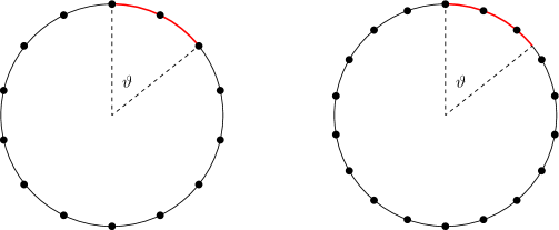
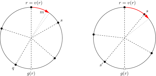
We will prove that Gathering is impossible for any given visibility range , provided that the size of the swarm is appropriate. Specifically, we say that a positive integer is compatible with if three conditions hold on the regular set of size (refer to Figure 1):
-
1.
For every , the open semicircle centered at contains exactly half of the points of .
-
2.
No two points of have an angular distance of exactly .
-
3.
There are two distinct points of whose angular distance is smaller than .
We can show that there are arbitrarily large such integers:
Proposition 3.1.
For any , there are arbitrarily large integers compatible with .
Proof 3.2.
It is easy to see that the first condition is satisfied if and only if is of the form , for some non-negative integer .
Let us turn to the second condition. The angular distance between two points of is a number of the form , for some positive integer . So, the second condition is satisfied if and only if there is no such that .
We will prove that, given any two integers of the form and , i.e., two consecutive numbers satisfying the first condition, at least one of them satisfies the second condition: this will allow us to conclude that there are arbitrarily large integers that satisfy both conditions (Figure 1 shows an example for ).
For the sake of contradiction, let us assume the opposite: there exists such that , and there exists such that . By combining the two equations, we have , or equivalently . The numbers and are two consecutive odd integers, and therefore they are relatively prime. It follows that must be a divisor of , and so . This implies that , contradicting the assumption that .
To satisfy the third condition, simply pick .
Choice of
For every integer compatible with , we define a positive number , which will be used to construct perturbations of the regular set of size . We set , where .
Since is compatible with , it easily follows that . Also, is at most half the angular distance between two consecutive points of , and therefore . Moreover, our choice of has some other desirable properties:
Proposition 3.3.
Let be an integer compatible with , let be the regular set of size , and let be an -perturbation of . If , and is the perturbed copy of , the following hold:
-
1.
The -neighborhood of contains a point if and only if the -neighborhood of contains the perturbed copy of in .
-
2.
The open semicircle centered at contains exactly half of the points of , which are the perturbed copies of the points of contained in .
-
3.
If is the open semicircle centered at , then , and hence contains exactly half of the points of .
Proof 3.4.
To prove the first statement, let and be the -neighborhoods of and , respectively. Let and be the endpoints of , such that , and let and be the endpoints of , such that . We have . Also, by definition of , for every point , we have , , , and . Moreover, if is the perturbed copy of , we have .
Suppose now that , and so . This means that , and also that , which in turn implies that . Conversely, if , we have , which leads to , and to , implying that .
The second and third statements are proved in a similar way. Note that, since is compatible with , contains exactly points of . Recall from the proof of Proposition 3.1 that is of the form , and therefore the smallest angular distance between a point of and an endpoint of is . Now we can repeat the proof of the first statement verbatim, with and instead of and , to conclude that a point lies in if and only if it lies in , which is true if and only if is the perturbed copy of a point of that lies in . Since , both and contain exactly points of .
Corollary 3.5.
Let be an integer compatible with , and let be an -perturbation of the regular set of size . If two swarms of robots form and respectively, their visibility graphs are isomorphic.
Proof 3.6.
The isomorphism is realized by mapping a robot in the first swarm, located in , to the robot in the second swarm located in the perturbed copy of . By the first statement of Proposition 3.3, there is an edge between two robots in the first swarm if and only if there is an edge between the corresponding robots in the second swarm.
Combining configurations
Next we will describe a way of combining two configurations of robots into a new one that takes an open semicircle from each. This operation will be used to construct configurations of robots where a given distributed algorithm fails to make the robots gather.
Let and be two subsets of , and let be an open semicircle. The -combination of and is defined as the set , where is the rotation of around the origin. In other words, this operation takes , discards the points that do not lie in , and replaces them with the points of that lie in , by mapping them to their antipodal points.
Preliminary lemmas
We are now ready to give our first two lemmas, which deal with swarms forming perturbations of a regular configuration, and analyze the distributed algorithms that make robots move in some ways. The first lemma states that, if an algorithm makes a robot move to a point not currently occupied by another robot, then the algorithm cannot solve the Gathering problem.
Lemma 3.7.
Let be a distributed algorithm, let be compatible with , and consider a swarm of robots that forms an -perturbation of the regular set of size . If there is a robot that, executing , moves to a point not in , then does not solve the Gathering problem, even under the condition that the swarm initially forms a rotationally asymmetric set of distinct points with a connected visibility graph.
Proof 3.8.
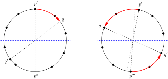
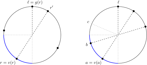
Let , and let be the open semicircle centered at . By the third statement of Proposition 3.3, . Assume that, if the robot located in executes , it moves to a point (see Figure 2 (left)). Let , and let be the -combination of and . Observe that, since , the -neighborhood of is a subset of , and therefore . Hence, , implying that .
Let be the antipodal point of . Note that the only points of whose antipodal points are not in are and . So, satisfies the hypotheses of Proposition 2.1, and therefore it is rotationally asymmetric.
Next we will prove that has a connected visibility graph. Let be the antipodal point of , let , and observe that is an -perturbation of the regular set of size . Since is compatible with , the -neighborhood of any point of contains at least two more points of , one on each side of it. It follows that the visibility graph of has a Hamiltonian cycle, and so does the visibility graph of , by Corollary 3.5. Hence, the visibility graph of has a Hamiltonian path. By the first statement of Proposition 3.3, the -neighborhood of any point of contains two more points of , one on each side of it. Therefore, each point of the circle lies in the -neighborhood of at least two points of . So, each point of lies in the -neighborhood of at least one point of . In particular, this is true of . We conclude that the visibility graph of contains a path connecting nodes (corresponding to ), plus a node (corresponding to ) connected to some node of , implying that the whole graph is connected.
Now, consider a swarm initially forming , which, as we recall, is a rotationally asymmetric set of distinct points with a connected visibility graph. Suppose that, in the first time unit, the scheduler activates only the robot in , which executes . Since the -neighborhood of is contained in , the robot gets the same snapshot as it would if the swarm’s configuration were . Therefore the robot moves to , and the swarm’s new configuration is . Observe that the antipodal of each point of is also in , and so any two antipodal points of have the same angle sequence. Due to Proposition 2.3, is rotationally symmetric, and hence is not a Gathering algorithm, by Corollary 2.7 (recall from Section 2 that, by definition, the existence of a single schedule that prevents the robots from gathering is sufficient to conclude that is not a Gathering algorithm).
The second lemma states that, if a distributed algorithm makes a robot move on top of another robot , and there is a perturbation of such that the same algorithm makes move on top of the same robot , then the algorithm does not solve the Gathering problem.
Lemma 3.9.
Let be a distributed algorithm, let be compatible with , let be the regular set of size , and let and be two distinct sets in the same bundle of -perturbations of , where and are the perturbed copies of . Assume that, if a swarm of robots forms and the robot in executes , it moves to another robot, located in . Also assume that, if a swarm of robots forms and the robot in executes , it moves to the same point . Then, does not solve the Gathering problem, even under the condition that the swarm initially forms a rotationally asymmetric set of distinct points with a connected visibility graph.
Proof 3.10.
Let be the open semicircle centered at , and let be the -combination of and . By the second statement of Proposition 3.3, , and so .
Since is compatible with , the visibility graph of is connected. Observe that is an -perturbation of , and so, by Corollary 3.5, its visibility graph is isomorphic to that of . This implies that the visibility graph of is connected, as well.
Let be the antipodal point of . Since , it follows that and are not antipodal to each other. Moreover, as and are in the same bundle of -perturbations of , we have . As a consequence, the only points of whose antipodal points are not in are and . So, satisfies the hypotheses of Proposition 2.1, and therefore it is rotationally asymmetric.
Consider a swarm initially forming , which, as we proved, is a rotationally asymmetric set of distinct points with a connected visibility graph. Suppose that, in the first time unit, the scheduler activates only the robots in and , which execute .
By the third statement of Proposition 3.3 applied to and (both of which are -perturbations of ), and since the -neighborhood of is contained in , the robot in gets the same snapshot as it would if the swarm’s configuration were . Hence, this robot moves to . Similarly, the robot in gets the same snapshot that it would if it were in and the swarm’s configuration were . So, this robot moves to , the antipodal point of . Since and are antipodal to each other, the swarm’s new configuration is a rotationally symmetric multiset, because each robot has an antipodal one with the same angle sequence, and therefore Proposition 2.3 applies. We conclude that is not a Gathering algorithm, due to Corollary 2.7.
Probabilistic argument
Our concluding argument goes as follows. Suppose for a contradiction that there is a Gathering algorithm for some . Let be an arbitrarily large integer compatible with , and let be the regular set of size . We will derive a contradiction by studying the behavior of on the swarms forming the -perturbations of . Specifically, let , , …, be the points of taken in clockwise order, starting from . Suppose that a swarm of robots forms a generic -perturbations of , with robot occupying the perturbed copy of , and let all robots execute algorithm .
Let us first restrict ourselves to a bundle of -perturbations of some , and let us analyze the possible behaviors of the robot . Recall that, by definition of bundle, the perturbations in have fixed coefficients for all the points of except , and perturb in every possible way by varying the coefficient . Observe that, by Lemma 3.7, should never make move to some unoccupied location, or would not be a Gathering algorithm. Also, if two or more perturbations in the bundle made move to the same robot, then would not be a Gathering algorithm, due to Lemma 3.9. However, by the pigeonhole principle, if perturbations in made move to some other robot, then at least two of them would make it move to the same robot. It follows that at most perturbations in can make move at all. So, all perturbations in except a finite number of them must make stay still.
Now, let us pick an -perturbation of by choosing its coefficients uniformly at random. Let us also define random variables , with , such that if and only if algorithm makes the robot stay still when the swarm’s configuration is the -perturbation of defined by the coefficients . By the above argument, for every bundle of -perturbations of , we have . Thus, with the convention that , we have
Hence, the probability that will make the robot stay still when the swarm’s configuration is picked at random among all -perturbations of is . Since this is true of all robots separately, it is also true of all robots collectively, by the inclusion-exclusion principle. In other words, with probability , on a random -perturbation of , no robot will be able to move, and therefore the robots will be unable to gather. Moreover, with probability , a random -perturbation of is rotationally asymmetric. As a consequence, there is at least one initial configuration (actually, a great deal of configurations) where the swarm forms a rotationally asymmetric set of distinct points with a connected visibility graph, and where no robot is able to move. We conclude that cannot be a Gathering algorithm, even under such strong conditions.
Technical obstacles
The probabilistic proof we outlined above is sound for the most part, but unfortunately making it rigorous is a delicate matter. The problem is that, in order for to be a random variable, it has to be a measurable function. For this to be true, the set of coefficients corresponding to perturbations where algorithm makes the robot stay still should be a measurable subset of . In turn, this requires some assumptions on the nature of , whereas we only defined as a generic function mapping a snapshot to a point.
However, since the function actually implements an algorithm, which typically is a finite sequence of operations that are well-behaved in an analytic sense, most reasonable assumptions on would rule out the pathological non-measurable cases, and would therefore make a properly defined random variable, allowing the rest of the proof to go through.
Nonetheless, we choose to adopt a different approach, which is both less technical and more general in scope. Indeed, we will give a “derandomized” version of the above proof, which will not deal with probability spaces and random variables, and will not require a more restrictive re-definition of which functions are computable by mobile robots.
Derandomization
Next we will show how to complete the previous argument without the use of probability. Note that we do not need to prove that a random perturbation causes all robots to stay still with probability : we merely have to show that there is at least one perturbation with such a property. This is significantly easier, and is achieved by the next lemma, where no longer denotes a random variable but simply a set of coefficients.
Lemma 3.11.
Let , and let , , …, be subsets of the unit hypercube such that every line parallel to the th coordinate axis intersects in less than points, for all . Then, there is a point in whose coordinates are all distinct that does not lie in any of the sets , , …, .
Proof 3.12.
For , let and let , with . Now let , and let . Observe that the sets are mutually disjoint, and therefore all the points of have distinct coordinates. We claim that contains a point that does not lie in any of the sets .
We will prove by induction on that, for all , the set contains a point that does not lie in . Thus, we will obtain our claim for .
To prove the base step, consider the set , with . This is a set of points lying on a line parallel to the first coordinate axis, and therefore it must contain a point that does not lie in .
For the inductive step, let , and consider the set , with . Since , we have . By the induction hypothesis, each of the sets of the form with contains a point not in . In other words, for each there exists such that the point is not in . Note that , and hence . So, by the pigeonhole principle, there exists such that there are at least different choices of for which the point is not in . Since these are at least points lying on a line parallel to the th coordinate axis, at least one of them does not lie in . It follows that such a point is in and does not lie in .
We can now prove the main result of this section.
Theorem 3.13.
If , and for arbitrarily large , there is no Gathering algorithm under the condition that the swarm initially forms a rotationally asymmetric set of distinct points with a connected visibility graph.
Proof 3.14.
Let be an arbitrarily large integer compatible with , which exists due to Proposition 3.1. Note that all -perturbations of the regular set of size have a connected visibility graph, by Corollary 3.5. As before, we assume for a contradiction that is a Gathering algorithm, and we consider a swarm of size where all robots execute , and each robot is initially located in the perturbed copy of point , for some -perturbation of .
For , let be the set of coefficients corresponding to perturbations where algorithm causes to make a non-null movement. As we already proved, due to Lemmas 3.7 and 3.9, in each bundle of -perturbations of , at most perturbations cause to move. Rephrased in geometric terms, every line in parallel to the th coordinate axis intersects in less than points.
So, the sets , , …, satisfy the hypotheses of Lemma 3.11 with . As a consequence, there exists , where the coefficients are all distinct, such that, in the perturbation corresponding to , algorithm causes all robots to stay still, and therefore does not allow them to gather.
It remains to check that the perturbation corresponding to is rotationally asymmetric. Let , , …, be the points of in clockwise order, and let be the perturbed copy of , for . Suppose for a contradiction that has a -fold rotational symmetry with , implying that the angular distance between and is . Note that is also the angular distance between and . Moreover, by definition of perturbation, . It follows that , which contradicts the fact that the coefficients are all distinct (indeed, implies that ).
We remark that, throughout the proofs of Lemmas 3.7, 3.9 and 3.13, only swarms of the same size appear. It follows that our impossibility result holds even if all robots know the size of the swarm.
4 Gathering algorithm for
Overview
In this section we give a Gathering algorithm for robots that can see the entire circle except their antipodal point (i.e., ), under the condition that the initial configuration is a rotationally asymmetric set with no multiplicity points.
First we will describe a simple Gathering algorithm for robots with full visibility, which already provides some useful ideas: elect a leader, form a unique multiplicity point, and gather there. We will then extend the same ideas to the limited-visibility case with . There are some difficulties arising from the fact that not all robots will necessarily agree on the same leader, because they may have different views of the rest of the swarm. For instance, two antipodal robots will not see each other, and, if the configuration is rotationally asymmetric, they will obtain two non-isometric snapshots, which may cause them to elect two different leaders.
We will show how to cope with these difficulties. Essentially, based on what a robot knows, there are only two possibilities on who the “true” leader may be, depending on whether there is a robot antipodal to or not. If happens to be elected leader in both scenarios, then has no doubt of being the leader, and therefore behaves as in the full-visibility algorithm, creating a multiplicity point. In most cases, however, no robot will be so fortunate, but the swarm will still have to make some sort of progress toward gathering. So, the robots that see themselves as possible leaders (but could be wrong) make some preparatory moves that will ideally “strengthen their leadership” in the next turns. We will argue that, after a finite number of turns, one robot will become aware of being the leader and will create a multiplicity point, even under a semi-synchronous scheduler.
The design and analysis of our Gathering algorithm are further complicated by some undesirable special cases, where two distinct multiplicity points end up being created, or the multiplicity point is antipodal to some robot, and therefore invisible to it.
Summary
This section is structured as follows. We begin by describing a simple algorithm for the full-visibility case, then proceed to the scenario where . In this context, we distinguish between the cognizant leader, i.e., a robot certain of its leadership, and the undecided leaders, i.e., robots that perceive themselves as leaders but are unsure due to incomplete information. Proposition 4.1 states that the true leader must belong to one of these two categories.
Next, we establish a technical result, Proposition 4.3, which supports the proof of the so-called point-addition lemma (Lemma 4.5). This crucial lemma describes a relationship between configurations that differ by only one robot; it leads to Corollary 4.7, which provides a non-trivial characterization of a cognizant leader.
These preliminary results pave the way for our Gathering algorithm, which consists of several numbered rules; any active robot applies a rule based on the configuration it observes. The rest of the section is dedicated to proving the correctness of this algorithm.
Lemma 4.9 establishes several constraints on which robots can execute certain rules and under what configurations. A notable implication of Lemma 4.9 is that only an undecided or cognizant leader may move (Corollary 4.11). Furthermore, Lemma 4.13 shows that at most two robots can move simultaneously, one of which is the true leader of the swarm.
These insights greatly simplify the analysis of potential executions of our Gathering algorithm. To begin with, it is relatively straightforward to prove that, if a multiplicity point is ever formed, the Gathering problem is eventually solved (Lemma 4.15). For all other scenarios, Lemma 4.17 shows that certain undesirable configurations do not occur as a result of executing the algorithm. Applying this knowledge, we establish that if a robot executes rule 3 or rule 4.a, the Gathering problem is eventually solved (Lemmas 4.19 and 4.21).
The rest of the analysis focuses on the remaining cases, where the only rules that are ever executed are rule 4.b and rule 4.c. Lemma 4.23 shows that under these rules, the configuration remains rotationally asymmetric without multiplicity points; Lemma 4.25 addresses the case where only the leader robot moves. Finally, Theorem 4.27 puts together all previous findings and concludes the proof of correctness.
Full visibility and leader election
We will describe a simple Gathering algorithm for the scenario where robots have full visibility.
Let be a rotationally asymmetric finite set of points on a circle. Recall from Proposition 2.3 that all points of have distinct angle sequences, and therefore there is a unique point with the lexicographically smallest angle sequence: is called the head of .
The Gathering algorithm uses the fact that all robots agree on where the head of the swarm is, and the robot located at the head is elected the leader. The algorithm makes the leader move clockwise to the next robot, while all other robots wait. As soon as there is a multiplicity point, the closest robot in the clockwise direction moves counterclockwise to the multiplicity point. The process continues until all robots have gathered.
Note that this algorithm also works in ASYNCH and with non-rigid robots (i.e., robots that can be stopped by an adversary before reaching their destination). Indeed, as the leader moves toward the next robot, its angle sequence remains the lexicographically smallest, and so it remains the leader. After a multiplicity point has been created, only one robot is allowed to move at any time, and therefore no other multiplicity points are accidentally formed.
Before delving into our main algorithm, we need definitions and lemmas that will justify some of our design choices.
Undecided leaders and cognizant leader
Let us now consider a swarm of robots with visibility range forming a rotationally asymmetric set of distinct points. We say that the true leader of the swarm is the robot located at the head of .
For each robot , we define the visible configuration as the set of robots that are visible to , and the ghost configuration as , with antipodal to . Note that exactly one between and is isometric to the “real” configuration , and therefore at least one between and is rotationally asymmetric.
The visible head is defined as follows: if is rotationally asymmetric, is the head of ; otherwise, is the head of . The ghost head is defined similarly: if is rotationally asymmetric, is the head of ; otherwise, is the head of . Note that the true leader of the swarm must be either or .
If , and either or , then is said to be an undecided leader: a robot that is possibly the true leader, but does not know for sure. If , then is a cognizant leader: a robot that is aware of being the true leader of the swarm.
Proposition 4.1.
In a rotationally asymmetric swarm with no multiplicity points, the true leader is either an undecided or a cognizant leader, and no robot other than the true leader can be a cognizant leader.
Proof 4.2.
Let the swarm form configuration , and let be the head of , i.e., the true leader. Either or , which means that either or : therefore, is an undecided or a cognizant leader.
Conversely, if a robot is a cognizant leader, then , implying that is the head of both and . But either or , and hence must be the head of , i.e., the true leader.
Point-addition lemma
We will now present some technical results that have important implications on the design of our Gathering algorithm. Although these results logically belong before the description of the algorithm itself, they may be skipped on a first reading, as they may be better appreciated after becoming familiar with the algorithm.
Proposition 4.3.
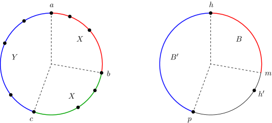
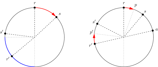
Let be a rotationally asymmetric finite set of points on a circle , let , and let , such that . If the angle sequence of truncated at is equal to the angle sequence of truncated at , then is not the head of .
Proof 4.4.
If and , we denote by the angle sequence of , and by the angle sequence of truncated at . Suppose for a contradiction that is the head of , and hence . Observe that , otherwise the hypotheses that and would imply that . As a consequence, the angle sequence is well defined, and so is for .
Note that the conditions on , , and imply that they are three distinct points, and that the clockwise arcs , , and are internally disjoint (refer to Figure 3 (left)). So, if we let and , we obtain , , and . Since is the head of , we have and . From the first inequality we derive , and from the second we derive , a contradiction.
Lemma 4.5.
Let be a finite non-empty set of points on a circle , and let , where . Assume that and are rotationally asymmetric, and let be the head of and be the head of . Then, either or .
Proof 4.6.
Let be the midpoint of the clockwise arc , i.e., . Let and . We have to prove that , as in Figure 3 (right). For the sake of contradiction, assume the contrary. Then, since , we have , as well as , because . It follows that . Let , with , be the angle sequence of with respect to , and let , with , be the angle sequence of with respect to . If , we define (respectively, ) as the angle sequence (respectively, ) truncated at .
Suppose first that , and note that . Let be such that , and observe that lies on the clockwise arc (possibly, ). Since , by Proposition 2.4 we have ; similarly, since , we have . Thus, . Observe that the hypotheses of Proposition 4.3 are satisfied by the set , with , , and . We conclude that is not the head of , a contradiction.
Suppose now that . Let be such that , and observe that does not lie on the clockwise arc (in particular, ). Since , by Proposition 2.4 we have ; similarly, since , we have . Thus, . Since , we must also have , otherwise we would have . Similarly, since , we must also have , otherwise we would have . So, , implying that , a contradiction.
Corollary 4.7.
In a rotationally asymmetric swarm with no multiplicity points, a robot is a cognizant leader if and only if .
Proof 4.8.
If is a cognizant leader, then obviously . For the converse, assume that . If or is rotationally symmetric, then by definition, and therefore is a cognizant leader. If and are rotationally asymmetric, we can apply Lemma 4.5 with and (and hence and ), obtaining either or . However, since , the second condition is impossible, because it implies that . It follows that , and so is a cognizant leader.
Gathering algorithm
Our Gathering algorithm for is illustrated in Listings 1, 4 and 5. A robot executing the algorithm first checks if the current configuration falls under some special cases (which will be discussed later), and then it attempts to determine the true leader of the swarm. By Corollary 4.7, checking if is equivalent to checking if is a cognizant leader. In this case, by Proposition 4.1, is the true leader, and hence it behaves like in the full-visibility algorithm: it moves clockwise to the next robot, (rule 3).
If is not a cognizant leader, it checks if it is at least an undecided leader: . In this case, cannot commit itself to moving to , because several robots may be undecided leaders, and this would create more than one multiplicity point. Instead, attempts to “strengthen its leadership” by moving halfway toward (rule 4.c): this ensures that, in the next turn, will have a lexicographically smaller angle sequence than it currently has (unless, of course, moves as well).
Another goal of is to be able to see the entire swarm in the next turns. Therefore, if the midpoint of and happens to be antipodal to some robot , then moves a bit further past the midpoint (rule 4.b). This way, will be sure to see in the next turn (unless, of course, moves as well).
An exception to the above is when is antipodal to , and has an antipodal robot . In this situation, if had an antipodal robot , then would be the true leader, which would then either form a multiplicity point with (if is activated) or would become visible to (if is activated but not ). However, if does not exist, then is the true leader, but may never find out: it may keep approaching without ever reaching it, and there may always be a ghost head antipodal to . For this reason, if detects this configuration, it moves slightly past (rule 4.a): this way, will be the new leader, and it will not be in the same undesirable configuration, because will not have an antipodal robot.
Note that, when describing rule 4.a and rule 4.b, we mentioned some undefined “small” distances. According to Listing 1, these are respectively and . In turn, is defined as the smallest angular distance between two points in , where is the set of all the points in plus their antipodal points. It is easy to see that all robots that are activated at the same time compute isometric sets , and therefore they implicitly agree on the value of . The reason why the specific values and have been chosen will become apparent in the proof of correctness of the algorithm.
Finally, let us discuss the special cases, all of which arise when some multiplicity points have been created (due to a cognizant leader moving to some other robot). If only one multiplicity point is visible to , then simply moves to it, as in the full-visibility algorithm (rule 1.a). In some exceptional circumstances, two multiplicity points and may be created, but we will prove that and will not be antipodal to each other, and there will never be a third multiplicity point. In this case, there is an implicit order between and on which all robots agree, and so they will all move to the same multiplicity point, say (rule 1.b). The last special case is when all robots have gathered in a point, except a single robot located in the antipodal point. detects this situation because it sees no robots other than itself (and its current location is not a multiplicity point). So, just moves to another visible point, say, the one forming a clockwise angle of with (rule 2). This ensures that will see the multiplicity point on its next turn.
Correctness
In the following, we will assume that all robots in a swarm of size execute the algorithm in Listing 1 starting from a rotationally asymmetric initial configuration with no multiplicity points. We will prove that, no matter how the adversarial semi-synchronous scheduler activates them, all robots will eventually gather in a point and no longer move.
We say that, in a given configuration , a robot is able to apply rule if, assuming that is activated when the swarm forms , executes rule (and no other rule).
Lemma 4.9.
Assume that the swarm forms a rotationally asymmetric configuration with no multiplicity points, and let be the true leader. Then:
-
1.
No robot is able to apply rule 1 or rule 2.
-
2.
At most one robot is able to apply rule 3: the true leader .
-
3.
At most one robot is able to apply rule 4.a: either the true leader (if there is no robot antipodal to ) or the robot antipodal to .
-
4.
A robot is able to apply rule 4 only if , and only if there is a robot antipodal to .
Proof 4.10.
To prove the first statement, observe that rule 1 and rule 2 only apply when there are multiplicity points, with one exception: when the swarm consists of exactly two robots, which are antipodal to each other. However, such a configuration is rotationally symmetric.
For the second statement, note that a robot is able to apply rule 3 only if , which, by Corollary 4.7, implies that is a cognizant leader. Therefore, by Proposition 4.1, .
To prove the third statement, assume that robot is able to apply rule 4.a, which means that and is antipodal to . Recall that either or . Specifically, if there is a robot in , then this robot is , and therefore is antipodal to . Otherwise there is no robot in , and so .
Let us now prove the fourth statement, which is illustrated in Figure 6 (left). Assume that a robot is able to apply rule 4, which means that , and therefore . Note that, since the true leader is , the swarm’s configuration is , and so there must be a robot antipodal to . Also, both and must be rotationally asymmetric, otherwise we would have , by definition of visible and ghost head. Thus, we can apply Lemma 4.5 with and (hence , , and ) to conclude that either (which is not the case) or . Since , we have . This inequality implies that lies on the clockwise arc , and therefore , or equivalently, . By plugging this into our last inequality, we obtain . Also, from the obvious fact that , we deduce that .
In light of Lemma 4.9, if the swarm forms a rotationally asymmetric configuration with no multiplicity points, we say that a robot is able to move if it is able to apply rule 3 or rule 4: indeed, these are the only rules that result in a non-null movement.
Corollary 4.11.
In any rotationally asymmetric configuration with no multiplicity points, a robot is able to move if and only if it is an undecided or a cognizant leader.
Proof 4.12.
By the first statement of Lemma 4.9, no robot is able to apply rule 1 or rule 2. Hence, a robot is able to apply rule 3 if and only if , and it is able to apply rule 4 if and only if . By Corollary 4.7, if and only if is a cognizant leader, and so if and only if is an undecided leader.
Lemma 4.13.
In any rotationally asymmetric configuration with no multiplicity points, at most two robots are able to move, and the true leader is always able to move.
Proof 4.14.
By Proposition 4.1, the true leader is either an undecided or a cognizant leader, and therefore, by Corollary 4.11, it is able to move.
Suppose for a contradiction that, in some rotationally asymmetric configuration with no multiplicity points, at least three distinct robots are able to move. One of these robots must be the true leader , hence there are two robots and , distinct from , that are able to move. Due to the second statement of Lemma 4.9, only is able to apply rule 3, and therefore and are able to apply rule 4. By the fourth statement of Lemma 4.9, we have and . It follows that the angular distance between and must be less than , and so, without loss of generality, we may assume that . In particular, and see each other, i.e., and . Refer to Figure 6 (right) for an example.
For any (respectively, ) and any point on the circle, we let (respectively, ) be the angle sequence of , with respect to (respectively, ), truncated at . Let be the point on the circle such that . Since is able to apply rule 4, we have , i.e., is the head of . In particular, and, by Proposition 2.4, . By a similar chain of deductions, since is able to apply rule 4, we have and . Recall that , and therefore , which implies that the antipodal points of and lie outside of the clockwise arc . But and only differ by the antipodal points of and , and so and . Thus, from we derive , which, together with , yields . Since is rotationally asymmetric (or else we would have ) and , it follows that satisfies the hypotheses of Proposition 4.3. We conclude that is not the head of , a contradiction.
Lemma 4.15.
If the swarm has a unique multiplicity point, then all robots eventually gather and no longer move.
Proof 4.16.
Let be the unique multiplicity point. Note that all robots are able to see and will move to it by rule 1.a when activated, except perhaps a single robot , antipodal to . If all robots except move to , while is not activated or only applies rule 5, then will eventually apply rule 2, moving to a different point. After that, will be able to see , and will move to it by rule 1.a.
Otherwise, if makes a move before all other robots are in , it does so by applying rule 3 or rule 4. If applies rule 4, then it will not create a new multiplicity point, all robots (including ) will thus see the unique multiplicity point , and will gather in it.
If applies rule 3, it moves to another robot ’s location. If is activated at the same turn, then moves to , no new multiplicity point is created, and all robots will eventually gather in . If is not activated at the same turn as , then will move to and create a new multiplicity point . Since rule 3 causes to move clockwise by an angle smaller than , we have . Now all robots see and perhaps also : either way, they will apply rule 1.a or rule 1.b, both of which result in a move to .
Lemma 4.17.
Assume that the swarm forms a rotationally asymmetric configuration with no multiplicity points, and let be a robot that is able to move. Then:
-
1.
If is activated and executes rule 4, then it moves by an angular distance strictly smaller than , and its destination point is not in , as defined in Listing 1.
-
2.
If is activated and executes rule 3, and is a robot that is able to move but is not activated, then does not move to .
-
3.
If both and are activated and execute rule 4.b or rule 4.c, then and are not antipodal to each other, and their destination points are not antipodal to each other.
Proof 4.18.
Since is able to move, by Corollary 4.11, it is either an undecided or a cognizant leader, implying that is the head of or of . Also, sees at least one other robot , or else it would be able to apply rule 2. If there is no robot such that , then the first element in the angle sequence of with respect to both and is at least . However, this also means that , and therefore has a lexicographically smaller angle sequence than with respect to both and , contradicting the fact that is the head of one of them. It follows that there must be some robot with . In particular, if is defined as in Listing 1, we have .
Let us prove the first statement: assume that executes rule 4, and let be its destination point. According to Listing 1, if executes rule 4.c, then and , implying that . If executes rule 4.b, then . By definition of , we have , and hence . This rule is executed only if the midpoint of and is . Since , then , by definition of . Finally, if executes rule 4.a, we have . Let be the antipodal point of , and note that, by definition of , we have . It follows that (note that we can write because is on the clockwise arc ). Moreover, since and , then we have , by definition of .
Let us prove the second statement, which is illustrated in Figure 7 (left). By repeating the above reasoning with , we infer that its next robot in the clockwise direction, , satisfies . If executes rule 3, then is the true leader, and , by Lemma 4.9. Thus, , implying that is distinct from the destination point of , because . We conclude that does not move to .
Let us now prove the third statement. Since both and are able to move, due to Lemma 4.13, one of them must be the true leader, say . By the fourth statement of Lemma 4.9, , and has an antipodal robot. Assume for a contradiction that is antipodal to . This means that coincides with the current configuration, and hence is the head of , i.e., . So, is able to apply rule 3, which contradicts the fact that it executes rule 4.b or rule 4.c. We have established that has no antipodal robot, and the robot antipodal to is (refer to Figure 7 (right)). Also, because , the robot is located in the interior of the clockwise arc . If is defined as in Listing 1, and is the destination point of , according to rule 4.b and rule 4.c, we have . So, the angular distance between and is smaller than . On the other hand, if is the destination point of , and is defined as above, we have . Hence, the angular distance between and is smaller than . By the triangle inequality, the angular distance between and is smaller than , implying that and are not antipodal to each other.
Lemma 4.19.
If the swarm forms a rotationally asymmetric configuration with no multiplicity points and an active robot executes rule 3, then all robots eventually gather in a point and no longer move.
Proof 4.20.
By Lemma 4.9, the robot that executes rule 3 must be the true leader , and any robot that moves at the same time as executes rule 4. Moreover, by Lemma 4.13, if such a robot exists, it is unique. According to rule 3, the destination point of is the location of another robot . So, if only moves, a unique multiplicity point is created on , and Lemma 4.15 allows us to conclude the proof.
Otherwise, assume that exists and moves at the same time as . By the second statement of Lemma 4.17, , and so still creates a multiplicity point on . On the other hand, by the first statement of Lemma 4.17, does not create a multiplicity point distinct from . Again, there is a unique multiplicity point, and we can apply Lemma 4.15.
Lemma 4.21.
If the swarm forms a rotationally asymmetric configuration with no multiplicity points and an active robot executes rule 4.a, then all robots eventually gather in a point and no longer move.
Proof 4.22.
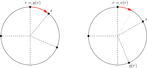
Let be the time at which some robot executes rule 4.a. By the third statement of Lemma 4.9, such a robot must be either the true leader or the robot antipodal to . If it is , we know by Lemma 4.13 that only and are able to move at time . However, in this case, is necessarily able to apply rule 3 at time : indeed, since has an antipodal robot, the current configuration coincides with , and therefore is the head of , i.e., . Thus, if is activated at time , it executes rule 3, and we conclude the proof by Lemma 4.19. So, if executes rule 4.a at time , we may assume that no other robot moves at the same time. On the other hand, if executes rule 4.a at time , by Lemmas 4.9 and 4.13 there is at most one other robot that is able to move at time . Such a robot is not antipodal to (otherwise would be able to execute rule 3, not rule 4.a), it is not able to execute rule 4.a (only or the robot antipodal to could), it has an antipodal robot , and .
In any case, we have the following situation at time (illustrated in Figure 8): a robot that executes rule 4.a (it does not matter if or ), and possibly another robot that executes rule 4.b or rule 4.c, with an antipodal robot , and such that (since is not antipodal to ). Let be the robot next to in the clockwise direction, and let . According to Listing 1, , there is a robot antipodal to , and , with antipodal to . Note that there is no robot such that , or else . We conclude that, whether is occupied by a robot or not, is the minimum angular distance between any two robots at time . Therefore, if is the robot next to in the clockwise direction, and , we have . On the other hand, we have by definition of . Let be computed as in Listing 1, and recall that all robots that are active at the same time agree on the same . Note that and . We distinguish three cases: (i) , (ii) , and (iii) does not exist.
(i) Let us first assume that at time (refer to Figure 8 (left)). Let us examine the configuration at time (hence, where referring to , we mean the position of at time , etc.). According to Listing 1, (rule 4.a), and either (rule 4.b) or (rule 4.c). The only exceptional case is , which implies that . In all cases, we have . Observe that no longer has an antipodal robot, and has moved by at least . It follows that is not antipodal to , and therefore has no antipodal robot, either. Moreover, implies that the angular distance between and is strictly smaller than any other, and in particular the configuration at time is still rotationally asymmetric, and is the new true leader. Also, all robots see both and (because and have no antipodal robots). So, the only robot such that is , and therefore no robot other than is able to move at time (recall that, due to the second statement of Lemma 4.9, if a robot other than the true leader is able to move, it must be able to apply rule 4). Moreover, the angular distance between the point antipodal to and the next robot in the clockwise direction, i.e., , is at least , which implies that . It follows that is able to apply rule 3 at time . So, the configuration will not change as long as is not activated, and eventually the semi-synchronous scheduler will activate . At that point, will execute rule 3, and Lemma 4.19 applies.
(ii) Let us now assume that at time (refer to Figure 8 (right)). From , we get , and so (recall that is the minimum angular distance between any two robots at time ). Also, since at time (or else would not be able to apply rule 4), and since sees both and , we have that (or else would not be the head of ). Hence, , implying that , and therefore does not move at time . Le us analyze the configuration at time . As in case (i), once again we have , and we can prove that the angular distance between and is strictly smaller than any other. In particular, the configuration at time is still rotationally asymmetric, and is the new true leader. Also, no robot other than can be antipodal to , by definition of and . But cannot be antipodal to either, because the point antipodal to satisfies , while . So, has no antipodal robots at time . However, unlike in case (i), still has an antipodal robot . Note that is able to apply rule 3, because , and so . All robots other that see both and , and are therefore unable to move at time . If is unable to move or is not activated before , then executes rule 3, and Lemma 4.19 applies.
So, we may assume that is the only robot to move, say, at time , when the configuration is still the same as at time . By the second statement of Lemma 4.9, must execute rule 4, and so at time . Let us prove that cannot apply rule 4.a. Assume the opposite, and let be the robot next to in the clockwise direction. According to Listing 1, must have an antipodal robot , and , because does not have an antipodal robot. Also, since there are no robots between and , we have . It follows that cannot be the head of , because it sees both and , and so has a lexicographically smaller angle sequence than with respect to . So, must execute either rule 4.b or rule 4.c at time , with . Let us consider the configuration at time . This is a situation analogous to case (i) at time : has executed rule 4.a with some , and has executed rule 4.b or rule 4.c with some . At this point, our previous argument repeats almost verbatim, with instead of and instead of : indeed, the only difference is that the inequality becomes .
(iii) Finally, let us assume that does not exist. At time , we have , and no robot other than has moved. This is analogous to the situation of case (ii) at time : indeed, the angular distance between and is the smallest, so the configuration is rotationally asymmetric, and is the true leader. Also, has an antipodal robot , and has no antipodal robot. From here, the proof proceeds verbatim as in case (ii).
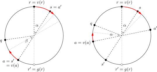
Lemma 4.23.
Assume that, at time , the swarm forms a rotationally asymmetric configuration with no multiplicity points, and all the robots that move at time execute rule 4.b or rule 4.c. Then, at time , the swarm still forms a rotationally asymmetric configuration with no multiplicity points.
Proof 4.24.
Due to Lemma 4.13, at most two robots and may move at time . If no robot moves at time , the configuration does not change, and there is nothing to prove. So, we have two cases: (i) only moves at time , and (ii) both and move at time .
(i) Suppose that only moves at time . Let be the next robot in the clockwise direction, and let be the destination point of . According to Listing 1, is in the interior of the clockwise arc , and hence there are no multiplicity points at time .
Assume for a contradiction that the configuration at time has a -fold rotational symmetry, with . According to Listing 1, at time , which implies that is the minimum angular distance between any two robots in at time . If no robot is antipodal to at time , then no two robots are closer than and . In this case, at time , and are strictly closer than any other pair of robots, which implies that , a contradiction.
So, we may assume that has an antipodal robot at time . Let (respectively, ) be the robot next to in the counterclockwise (respectively, clockwise) direction. Note that at time includes all robots except . So, at time , is strictly smaller than the angular distance between any two robots, except perhaps and or and .
Let us discuss all possibilities for , , and at time (refer to Figure 9 (left)). If one among , , or is smaller than the other two, then there is a unique pair of robots that is strictly closer than any other pair, which implies that , a contradiction. If , then there are exactly three pairs of robots that are closest to each other, and therefore . This means that the rotational symmetry maps to , to , and to . In particular, we have at time , which contradicts the fact that and .
Finally, if two among , , and are equal and the third one is greater, then there are exactly two pairs of robots that are closest to each other, and therefore , i.e., the rotational symmetry exchanges the two pairs. If , the rotational symmetry should map to , which is impossible because and are not antipodal to each other. If , the rotational symmetry maps to , contradicting the fact that they are not antipodal to each other. Similarly, if , the rotational symmetry maps to , which is impossible because they are not antipodal to each other at time .
(ii) Assume that both and move at time , as in Figure 9 (right). By Lemma 4.13, one of the two robots, say , is the true leader. So, if is the robot next to in the clockwise direction, then is the minimum angular distance between any two robots at time . By the fourth statement of Lemma 4.9, we have . On the other hand, by the third statement of Lemma 4.17, and are not antipodal to each other, and so . It follows that , or else would have an angle sequence lexicographically smaller than , contradicting the fact that is the true leader.
Let and be the destination points of and , respectively. According to Listing 1, is in the interior of the clockwise arc , and is in the interior of the clockwise arc , where is the robot next to in the clockwise direction. Since the two arcs are internally disjoint, we have , and therefore there are no multiplicity points at time .
Assume for a contradiction that the configuration at time has a -fold rotational symmetry, with . Note that, since , the robot does not move at time . Therefore, at time , is strictly smaller than the angular distance between any two robots, except perhaps and . If at time , then and are strictly closer than any other pair of robots, implying that , a contradiction. Similarly, if at time , then and are strictly closer than any other pair of robots, and once again we have . On the other hand, if at time , then there are exactly two pairs of robots that are closest to each other, and therefore , i.e., the rotational symmetry exchanges the two pairs. We conclude that and are antipodal to each other at time , or, equivalently, and are antipodal to each other. However, since both and executed rule 4.b or rule 4.c at time , this contradicts the third statement of Lemma 4.17.
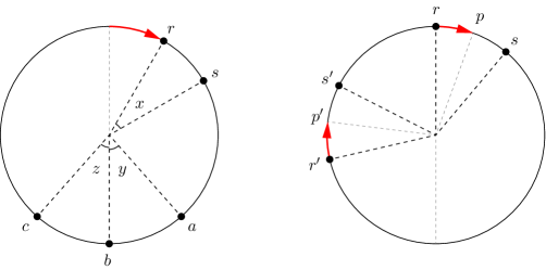
Lemma 4.25.
Assume that, at time , the swarm forms a rotationally asymmetric configuration with no multiplicity points. If, at all times , no robot other than the true leader moves (either because it is unable to move or because it is not activated), then all robots eventually gather in a point and no longer move.
Proof 4.26.
By Lemma 4.13, the true leader must be able to move at time . Let be the robot next to in the clockwise direction, and observe that the angular distance between and at time is not greater than the angular distance between any two robots in the swarm (or else, would not have the lexicographically smallest angle sequence). As long as is not activated, the configuration will remain the same, and will remain the true leader. The semi-synchronous scheduler will eventually activate , say at time , and hence will execute either rule 3 (in which case we conclude the proof by Lemma 4.19) or rule 4.a (in which case we conclude the proof by Lemma 4.21), or rule 4.b or rule 4.c. In the latter two cases, the angular distance between and is reduced by at least one half, and so it becomes strictly smaller than the angular distance between any other pair of robots. It follows that the configuration at time is still rotationally asymmetric, and is still the true leader.
By inductively applying the same reasoning as above, we argue that either all robots gather in a point and no longer move, or there is an increasing sequence such that, for every , at time the robot executes rule 4.b or rule 4.c, the angular distance between and is reduced by at least one half, and remains the true leader. So, if is the value of at time , we have , that is, keeps approaching indefinitely.
Let be a large-enough index such that, at time , the angle is strictly smaller than half the angular distance between any robot other than and its next robot clockwise. Let be the set at time . If is rotationally symmetric, then is a cognizant leader at time (by definition of and ), and therefore it executes rule 3, due to Corollary 4.7. In this case we can apply Lemma 4.19, so we may assume that is rotationally asymmetric, and therefore it has a head . Since both and are in , there must be a point such that . So, there are only two possibilities for the location of : either or the point antipodal to (in which case must be the point antipodal to ). If is the head of , then at time it executes rule 3, and we can apply Lemma 4.19. Otherwise, if the point antipodal to is the head of , it means that has an antipodal robot. So, executes rule 4.a at time , and we conclude the proof by Lemma 4.21.
We are now ready to prove the main result of this section.
Theorem 4.27.
If , there is a Gathering algorithm under the condition that the swarm initially forms a rotationally asymmetric configuration with no multiplicity points.
Proof 4.28.
We will prove that the distributed algorithm in Listing 1 solves the Gathering problem under the condition that the swarm initially forms a rotationally asymmetric configuration with no multiplicity points. By the first statement of Lemma 4.9, whenever the swarm forms a rotationally asymmetric configuration with no multiplicity points, any robot that is activated and moves executes either rule 3 (in which case we conclude the proof by Lemma 4.19), or rule 4.a (in which case we conclude the proof by Lemma 4.21), or rule 4.b, or rule 4.c. In the latter two cases, by Lemma 4.23, the resulting configuration is still rotationally asymmetric and with no multiplicity points. By inductively repeating this argument, we may assume, without loss of generality, that the swarm forms a rotationally asymmetric configuration with no multiplicity points at all times, and all robots that are activated and move execute rule 4.b or rule 4.c.
By Lemma 4.13, at a generic time , at least one robot and at most one other robot are allowed to move. The semi-synchronous scheduler will activate each of them infinitely often, so let be the first time at least one of them is activated. Assume that one robot, say , is not activated at time , and therefore is. Then, does not have an antipodal robot at time , due to the first statement of Lemma 4.17. Similarly, if both and are activated at time , none of them has an antipodal robot at time , by the first and third statements of Lemma 4.17.
In summary, if a robot is activated and moves at a generic time , it no longer has antipodal robots at any time after . Since the robots are finitely many, eventually, say after time , only robots without an antipodal robot will move. However, by the fourth statement of Lemma 4.9, a robot that moves must have an antipodal robot, unless it is the current true leader. So, at all times after , no robot other than the current true leader will move. Therefore, Lemma 4.25 allows us to conclude the proof.
5 Conclusions
Summary
We gave a deterministic distributed algorithm to solve the Gathering problem on a circle for semi-synchronous rigid mobile robots with chirality (under the necessary condition that the initial configuration is rotationally asymmetric), assuming that each robot can see the entire circle except its antipodal point, i.e., for . On the other hand, we proved that no such algorithm exists if , even if the robots know the size of the swarm, and even if the initial configuration is rotationally asymmetric and has a connected visibility graph. We remark that the latter impossibility result is not limited to the Gathering problem, but extends to all Pattern Formation problems where the pattern is rotationally asymmetric.
Open problems
By inspecting the proof of correctness of our Gathering algorithm for , it is easy to see that its running time is epochs, where is the total number of robots, and an “epoch” is defined as a minimal timespan where every robot is activated at least once. Indeed, the only step that may take a non-constant number of epochs is discussed in the proof of Theorem 4.27, where a termination condition occurs as soon as a multiplicity point appears or no robots are antipodal to each other. In principle, this could take epochs in the worst case, but we do not have a concrete example where it actually takes that long. In fact, we believe that our algorithm terminates in epochs, but a deeper analysis is needed to confirm this conjecture.
Note that the technique of our impossibility proof is ineffective when , because it relies on the fact that a robot’s snapshot is contained in an open semicircle, which in turn enables combining snapshots as a means to construct configurations where Gathering is impossible. We leave the design of Gathering algorithms or proofs of impossibility for these remaining cases as an open problem.
Other natural open problems concern the relaxation of some of our assumptions concerning the capabilities of the robots and the scheduler. For instance, we can prove that, under an asynchronous scheduler, the algorithm in Listing 1 may cause the swarm to partition into two antipodal multiplicity points: a configuration from which Gathering cannot be achieved. Our question is whether a Gathering algorithm exists for an asynchronous scheduler if .
Similarly, removing the rigidity condition may cause the formation of two antipodal multiplicity points. For example, a robot executing rule 4.a may end up stopping on the next robot instead of slightly past it. If has an antipodal robot , then will move to the next robot , creating two antipodal multiplicity points at and . It is an open problem whether non-rigid robots can solve the Gathering problem with . A related question is whether the chirality assumption can be removed.
Another interesting problem concerns the necessity of (weak) multiplicity detection. It is not clear if the Gathering problem can be solved at all by robots with no multiplicity detection. On the other hand, assuming that the initial configuration has no multiplicity points essentially serves to prevent the occurrence of antipodal multiplicity points. It is an open problem whether this condition can be relaxed somehow.
Conversely, there are open problems arising from robot models with additional capabilities. For example, we may wonder if a fully synchronous scheduler (which activates all robots at all times) allows for simpler or improved Gathering algorithms. Another intriguing question is whether the knowledge of the size of the swarm and stronger multiplicity detection would help in the design of a Gathering algorithm for a large-enough .
Finally, the presence of colored lights is a feature that is worth investigating. In this model, each robot is able to signal information (usually only a few bits) to all visible robots by means of a colored light. Since our impossibility result does not hold in this model, we wonder if colored lights may allow robots to gather when their visibility range is shorter than , or even shorter than . Colored lights may also be traded with chirality, rigidity, or synchrony.
References
- [1] N. Agmon and D. Peleg. Fault-tolerant gathering algorithms for autonomous mobile robots. SIAM Journal on Computing, 36(1):56–82, 2006.
- [2] H. Ando, Y. Oasa, I. Suzuki, and M. Yamashita. Distributed memoryless point convergence algorithm for mobile robots with limited visibility. IEEE Transactions on Robotics and Automation, 15(5):818–838, 1999.
- [3] S. Bhagat, K. Mukhopadhyaya, and S. Mukhopadhyaya. Computation under restricted visibility. In Distributed Computing by Mobile Entities: Current Research in Moving and Computing, pages 134–183. Springer, 2019.
- [4] J. Castenow, J. Harbig, D. Jung, P. Kling, T. Knollmann, and M. Meyer auf der Heide. A unifying approach to efficient (near)-gathering of disoriented robots with limited visibility. In 26th International Conference on Principles of Distributed Systems,, pages 15:1–15:25, 2022.
- [5] M. Cieliebak, P. Flocchini, G. Prencipe, and N. Santoro. Distributed computing by mobile robots: gathering. SIAM Journal on Computing, 41(2):829–879, 2012.
- [6] P. Courtieu, L. Rieg, S. Tixeuil, and X. Urbain. Impossibility of gathering, a certification. Information Processing Letters, 115(3):447–452, 2015.
- [7] J. Czyzowicz, D. Ilcinkas, A. Labourel, and A. Pelc. Asynchronous deterministic rendezvous in bounded terrains. In 17th International Colloquium on Structural Information and Communication Complexity, pages 72–85, 2010.
- [8] J. Czyzowicz, A. Kosowski, and A. Pelc. Deterministic rendezvous of asynchronous bounded-memory agents in polygonal terrains. Theory of Computing Systems, 52(2):179–199, 2013.
- [9] J. Czyzowicz, A. Pelc, and A. Labourel. How to meet asynchronously (almost) everywhere. ACM Transactions on Algorithms, 8(4):231–261, 2012.
- [10] G. D’Angelo, G. Di Stefano, and A. Navarra. Gathering on rings under the Look–Compute–Move model. Distributed Computing, 27(4):255–285, 2014.
- [11] G. D’Angelo, A. Navarra, and N. Nisse. A unified approach for gathering and exclusive searching on rings under weak assumptions. Distributed Computing, 30(1):17–48, 2017.
- [12] X. Défago, M. Gradinariu, S. Messika, P. Raipin-Parvédy, and S. Dolev. Fault-tolerant and self-stabilizing mobile robots gathering. In 20th International Symposium on Distributed Computing, pages 46–60, 2006.
- [13] B. Degener, B. Kempkes, P. Kling, F. Meyer auf der Heide, P. Pietrzyk, and R. Wattenhofer. A tight runtime bound for synchronous gathering of autonomous robots with limited visibility. In 23rd ACM Symposium on Parallelism in Algorithms and Architectures, pages 139–148, 2011.
- [14] G.A. Di Luna, P. Flocchini, L. Pagli, G. Prencipe, N. Santoro, and G. Viglietta. Gathering in dynamic rings. Theoretical Computer Science, 811:79–98, 2020.
- [15] G.A. Di Luna, P. Flocchini, N. Santoro, and G. Viglietta. TuringMobile: a turing machine of oblivious mobile robots with limited visibility and its applications. In 32nd International Symposium on Distributed Computing, pages 19:1–19:18, 2018.
- [16] G.A. Di Luna, P. Flocchini, N. Santoro, G. Viglietta, and M. Yamashita. Meeting in a polygon by anonymous oblivious robots. In 31st International Symposium on Distributed Computing, pages 14:1–14:15, 2017.
- [17] G.A. Di Luna, R. Uehara, G. Viglietta, and Y. Yamauchi. Gathering on a circle with limited visibility by anonymous oblivious robots. In 34th International Symposium on Distributed Computing, pages 12:1–12:17, 2020.
- [18] P. Flocchini. Gathering. In Distributed Computing by Mobile Entities: Current Research in Moving and Computing, pages 63–82. Springer, 2019.
- [19] P. Flocchini, R. Killick, E. Kranakis, N. Santoro, and M. Yamashita. Gathering and election by mobile robots in a continuous cycle. In 30th International Symposium on Algorithms and Computation, pages 8:1–8:19, 2019.
- [20] P. Flocchini, G. Prencipe, and N. Santoro. Self-deployment of mobile sensors on a ring. Theoretical Computer Science, 402(1):67–80, 2008.
- [21] P. Flocchini, G. Prencipe, and N. Santoro. Distributed Computing by Oblivious Mobile Robots. Morgan & Claypool, 2012.
- [22] P. Flocchini, G. Prencipe, and N. Santoro, editors. Distributed Computing by Mobile Entities, Current Research in Moving and Computing. Springer, 2019.
- [23] P. Flocchini, G. Prencipe, N. Santoro, and G. Viglietta. Distributed computing by mobile robots: uniform circle formation. Distributed Computing, 30(6):413–457, 2017.
- [24] P. Flocchini, G. Prencipe, N. Santoro, and P. Widmayer. Gathering of asynchronous robots with limited visibility. Theoretical Computer Science, 337(1–3):147–168, 2005.
- [25] N. Fujinaga, Y. Yamauchi, S. Kijima, and M. Yamahista. Pattern formation by oblivious asynchronous mobile robots. SIAM Journal on Computing, 44(3):740–785, 2015.
- [26] S. Guilbault and A. Pelc. Gathering asynchronous oblivious agents with local vision in regular bipartite graphs. Theoretical Computer Science, 509:86–96, 2013.
- [27] E. Huus and E. Kranakis. Rendezvous of many agents with different speeds in a cycle. In 14th International Conference on Ad-Hoc, Mobile, and Wireless Networks, pages 195–209, 2015.
- [28] S. Kamei, A. Lamani, and F. Ooshita. Asynchronous ring gathering by oblivious robots with limited vision. In 33rd International Symposium on Reliable Distributed Systems, pages 46–49, 2014.
- [29] S. Kamei, A. Lamani, F. Ooshita, S. Tixeuil, and K. Wada. Gathering on rings for myopic asynchronous robots with lights. In 23rd International Conference on Principles of Distributed Systems, pages 27:1–27:17, 2019.
- [30] Y. Kim, M. Shibata, Y. Sudo, J. Nakamura, Y. Katayama, and T. Masuzawa. Gathering of mobile robots with defected views. In 26th International Conference on Principles of Distributed Systems,, pages 14:1–14:18, 2022.
- [31] R. Klasing, E. Markou, and A. Pelc. Gathering asynchronous oblivious mobile robots in a ring. Theoretical Computer Science, 390(1):27–39, 2008.
- [32] E. Kranakis, D. Krizanc, F. MacQuarrie, and S.M. Shende. Randomized rendezvous algorithms for agents on a ring with different speeds. In 16th International Conference on Distributed Computing and Networking, pages 9:1–9:10, 2015.
- [33] E. Kranakis, D. Krizanc, and E. Markou. The Mobile Agent Rendezvous Problem in the Ring. Morgan and Claypool, 2010.
- [34] A. Monde, Y. Yamauchi, S. Kijima, and M. Yamashita. Self-stabilizing localization of the middle point of a line segment by an oblivious robot with limited visibility. In 19th International Symposium on Stabilization, Safety, and Security of Distributed Systems, pages 172–186, 2017.
- [35] L. Pagli, G. Prencipe, and G. Viglietta. Getting close without touching: near-gathering for autonomous mobile robots. Distributed Computing, 28(5):333–349, 2015.
- [36] P. Poudel and G. Sharma. Universally optimal gathering under limited visibility. In 19th International Symposium on Stabilization, Safety, and Security of Distributed Systems, pages 323–340, 2017.
- [37] S. Souissi, X. Défago, and M. Yamashita. Using eventually consistent compasses to gather memory-less mobile robots with limited visibility. ACM Transactions on Autonomous and Adaptive Systems, 4(1):9:1–9:27, 2009.
- [38] I. Suzuki and M. Yamashita. Distributed anonymous mobile robots: formation of geometric patterns. SIAM Journal on Computing, 28(4):1347–1363, 1999.
- [39] Y. Yamauchi. Symmetry of anonymous robots. In Distributed Computing by Mobile Entities, Current Research in Moving and Computing, pages 109–133. Springer, 2019.
- [40] Y. Yamauchi, T. Uehara, S. Kijima, and M. Yamashita. Plane formation by synchronous mobile robots in the three-dimensional euclidean space. Journal of the ACM, 64(3):16:1–16:43, 2017.
- [41] Y. Yamauchi and M. Yamashita. Pattern formation by mobile robots with limited visibility. In 20th International Colloquium on Structural Information and Communication Complexity, pages 201–212, 2013.