∎

¹¹institutetext: P. Arrighi ²²institutetext: N. Eon (²²email: nathanael.eon@lis-lab.fr) ³³institutetext: Aix-Marseille Université, Université de Toulon, CNRS, LIS, Marseille, France ⁴⁴institutetext: G. Di Molfetta ⁵⁵institutetext: Université Publique, CNRS, LIS, Marseille, France and Quantum Computing Center, Keio University, 3-14-1 Hiyoshi, Yokohama, Kanagawa, 223-8522, Japan

Gauge-invariance in cellular automata

Pablo Arrighi Giuseppe Di Molfetta Nathanaël Eon

(6 January 2022)

Abstract

Gauge-invariance is a fundamental concept in Physics—known to provide mathematical justification for the fundamental forces. In this paper, we provide discrete counterparts to the main gauge theoretical concepts directly in terms of Cellular Automata. More precisely, the notions of gauge-invariance and gauge-equivalence in Cellular Automata are formalized. A step-by-step gauging procedure to enforce this symmetry upon a given Cellular Automaton is developed, and three examples of gauge-invariant Cellular Automata are examined.

Keywords:

Gauge-invariance Cellular Automata Quantum Cellular Automata

^†^†journal: Natural Computing

1 Introduction

In Physics, symmetries are essential concepts used to derive the laws which model nature. Among them, gauge symmetries are central, since they provide the mathematical justification for all four fundamental interactions: the weak and strong forces (short range interactions), electromagnetism quigg2013gauge and to some extent gravity (long range interactions). In Computer Science, cellular automata (CA) constitute the most established model of computation that accounts for euclidean space. Yet its origins lies in Physics, where they were first used to model hydrodynamics and multi-body dynamics, and are now commonly used to model particles or waves. In this paper, the key notions of gauge-invariance are defined in the discrete model of CA, and a counterpart to the gauging procedure—a step-by-step method to enforce this symmetry—is formalized within CA.

These methods may lead to natural, Physics-inspired CA. More importantly, the fields of numerical analysis, quantum simulation, digital Physics are constantly looking for discrete schemes that simulate known Physics georgescu2014quantum ; notarnicola2020real . Quite often, these discrete schemes seek to retain the symmetries of the simulated Physics; whether in order to justify the discrete scheme as legitimate, or in order to do the Monte Carlo-counting right hastings1970monte . Generally speaking, since gauge symmetries are essential in Physics, having a discrete counterpart of it may also be Arrighi2020 .

Interestingly, this way of enforcing local redundancies also bears some resemblances with error-correction, as was pointed out in the context of quantum computation in kitaev2003fault ; nayak2008non , and echoes the fascinating question of noise resistance within spatially distributed models of computation harao1975fault ; Toom .

Although we authors come from the field of quantum computation and simulation, the formalism we use is totally devoid of least action principle, or Lagrangian. The notions here are directly formulated in terms of the discrete dynamical system. We believe that this provides a uniquely direct route to the root concepts. This discrete mathematics framework makes the presentation original, and simpler. But it also allows for more rigorous definitions, that in turn allow us to prove an equivalence lemma.

This work is based on two previous conference papers arrighi2018gauge ; arrighi2019non by the authors. It also integrates a quantum example Arrighi2020 by one of the authors. The examples expressed here provide what seems to be the simplest non-trivial Gauge theories so far and illustrates the key concepts. Given that Gauge theories are infamously difficult, we think this may be a remarkable pedagogical asset.

The paper is organized as follows. In Sec. 2 we introduce the formal definitions of cellular automata—both classical and quantum— and the notions of gauge transformations and gauge symmetry. In Sec. 3, a discrete counterpart to the gauging procedure is developed and illustrated through a simple example. It provides the route one may take in order to obtain a gauge-invariant CA, starting from one that does not implement the symmetry. Sec. 4 goes through three examples of gauge-invariant CA from the literature given in the same framework: a very simple classical version arrighi2018gauge , a generalization to a larger type of gauge transformations arrighi2019non , and a quantum CA (QCA) Arrighi2020 . In Sec. 5, the notion of equivalence between gauge-invariant CA is formalized and characterized. In Sec. 6 we summarize, provide related works and perspectives.

2 Definitions

2.1 Cellular automata

A cellular automaton (CA) is a dynamical system which operates on a discrete, uniform space and evolves in discrete time steps through the application— homogeneously across space—of a local operator. Let us make this formal.

Notations.

For the reader who does not need any reminder about CA, here is a list of notations which will be used in the following:

•

${\mathbb{Z}^{d}}$ : underlying structure of space with dimension $d$ .
•

$\Sigma$ : alphabet.
•

${\mathcal{C}}=\Sigma^{\mathbb{Z}^{d}}$ : set of all configurations.
•

${\mathcal{N}}$ : neighbourhood.
•

$c_{x}$ for $c\in{\mathcal{C}}$ and $x\in{\mathbb{Z}^{d}}$ : shorthand for $c(x)$
•

$c_{t,x}$ for $c\in{\mathcal{C}}$ , $x\in{\mathbb{Z}^{d}}$ and $t\in\mathbb{N}$ : shorthand for $\big{(}F^{t}(c)\big{)}_{x}$
•

$c_{|I}$ for $c\in{\mathcal{C}}$ and $I\subset{\mathbb{Z}^{d}}$ : shorthand for $c:I\longrightarrow\Sigma$ the configuration restricted to a set $I$ of specific positions.

Space-time representation.

The discrete, uniform space on which CA are based, is usually the grid ${\mathbb{Z}^{d}}$ with $d$ the dimension—although more general definitions exist, that replace the grid by bounded degree graphs, typically Cayley graphs. The results will be given for ${\mathbb{Z}^{d}}$ with $d$ the dimension, and our examples will only be in one-dimension ( $d=1$ ) for simplicity.

Alphabet and classical configuration.

The alphabet $\Sigma$ is a countable—often finite—set.

Definition 1 (Classical configuration).

A classical configuration $c$ over an alphabet $\Sigma$ is a function that associates a state to each point in ${\mathbb{Z}^{d}}$ :

c:{\mathbb{Z}^{d}}\longrightarrow\Sigma.

(1)

The set of all configurations will be denoted $\mathcal{C}$ .

A configuration should be seen as the state of the CA at a given time. We use the shorthand notation $c_{x}=c(x)$ for $x\in{\mathbb{Z}^{d}}$ and $c_{|I}$ for the configuration $c$ restricted to the set $I$ —i.e. $c:I\longrightarrow\Sigma$ —for $I\subset{\mathbb{Z}^{d}}$ . The association of a position and its state is called a cell.

Local rule.

Now that we have a way to describe the system at a given time—using a configuration—we should define the local rule. A neighbourhood is a finite subset of ${\mathbb{Z}^{d}}$ , which is denoted ${\mathcal{N}}$ . The local rule takes as input a configuration restricted to the neighbourhood ${\mathcal{N}}$ of a cell and outputs the next value of the cell.

f:\Sigma^{{\mathcal{N}}}\longrightarrow\Sigma.

(2)

Applying this local rule at every position simultaneously defines the evolution of a configuration.

Definition 2 (Cellular Automaton).

A cellular automaton $F$ with alphabet $\Sigma$ , dimension $d$ and neighbourhood ${\mathcal{N}}$ is a function $F:\mathcal{C}\longrightarrow\mathcal{C}$ to another configuration by applying a local rule $f:\Sigma^{\mathcal{N}}\longrightarrow\Sigma$ at every position synchronously:

F(c)_{i}=f(c_{|i+{\mathcal{N}}})

(3)

where $i\in{\mathbb{Z}^{d}}$ .

Because the CA defines the configuration at time $t+1$ knowing the configuration at time $t$ , we will denote by $c_{t,x}$ the value of a cell at position $x$ and time $t$ .

2.2 Quantum cellular automata

The definition of QCA used here is commonly known as partitioned QCA (PQCA) schumacher2004reversible ; arrighi2019overview . This choice is motivated by the similarity with the classical version while not loosing any generality due to the intrinsically universal nature of PQCA arrighi2012partitioned .

Hilbert space of quantum configurations

The quantum configurations differ from classical configurations because they require a distinguished element of $\Sigma$ to be called the empty state and such that only a finite number of cells are not empty.

Definition 3 (Finite unbounded configurations).

Consider $\Sigma$ the alphabet, with $0$ a distinguished element of $\Sigma$ , called the empty state. A finite unbounded configuration $c$ over $\Sigma$ is a function $c:\mathbb{Z}^{d}\longrightarrow\Sigma$ , such that the set of the $(i_{1},\ldots,i_{d})\in\mathbb{Z}^{d}$ for which $c_{i_{1}\ldots i_{d}}\neq 0$ , is finite. The set of all finite unbounded configurations will be denoted $\mathcal{C}_{f}$ .

The finite unbounded configurations are taken as basis to build the Hilbert space of configurations which allows for superposition of configurations.

Definition 4 (Hilbert space of configurations).

The Hilbert space of configurations is that having orthonormal basis $\{\ket{c}\}_{c\in\mathcal{C}_{f}}$ . It will be denoted $\mathcal{H}$ .

PQCA.

A PQCA works by partitioning the space into supercells, applying a local unitary operator $U$ on those supercells, and then doing so again at shifted positions.

Definition 5 (PQCA).

A $d$ -dimensional partitioned QCA (PQCA) $G$ is induced by a scattering unitary $U$ taking a hypercube of $2^{d}$ cells into a hypercube of $2^{d}$ cells, i.e. acting over $\mathcal{H}_{\Sigma}^{\otimes 2^{d}}$ , and preserving quiescence, i.e. $U\ket{0\ldots 0}=\ket{0\ldots 0}$ . Let $J=(\bigotimes_{2\mathbb{Z}^{d}}U)$ over $\mathcal{H}$ and $\tau=\tau_{1}\ldots\tau_{d}$ the diagonal translation. The induced global evolution is $J$ at even steps, and $\tau^{\dagger}J\tau$ at odd steps.

The local unitary $U$ in a PQCA can be thought of as a reversible version of the local function $f$ of a classical CA.

2.3 Gauge-invariance in CA.

Gauge transformations.

A global gauge transformation is a function that maps configurations to configurations through the application of a position-dependent, local gauge transformation at every position.

Definition 6 (Local gauge transformation group).

Let $s\in\mathbb{N}$ be the radius. A group $G$ of local gauge transformations with alphabet $\Sigma$ , radius $s$ and space dimension $d$ is a subgroup of the bijections over $\Sigma^{(2s+1)^{d}}$ with further requirement that any two local gauge transformations, applied at distinct positions on words of size $(4s+1)^{d}$ , commute. It is extended to act upon $\mathcal{H}_{\Sigma^{(2s+1)^{d}}}$ ) by linearity.

We shall use the abuse of notation $g_{x}\in G$ for a local gauge transformation over $\mathcal{C}$ (or $\mathcal{H}$ in the quantum case) where the local transformation is applied around the cell at position $x$ , i.e. on the cells at positions $\{x-s,\ldots,x+s\}$ , and is the identity everywhere else.

In the following, local gauge transformations will refer to the classical or quantum case depending on the context.

Definition 7 (Global gauge transformation).

Let $\Sigma$ be the alphabet, $s\in\mathbb{N}$ the radius, $d$ the dimension and $G$ a local gauge transformation group with respect to these $\Sigma$ , $s$ and $d$ . A function $\gamma$ is a gauge transformation with respect to the local gauge transformation group $G$ if there exists a family $(g_{x})_{x\in{\mathbb{Z}^{d}}}$ of elements of $G$ such that:

\gamma=\prod_{x\in\mathbb{Z}^{d}}g_{x}

(4)

and this product is unambiguous, because for any $x,y$ in ${\mathbb{Z}^{d}}$ , with $x\neq y$ , the following commutation relation holds $[g_{x},g_{y}]=0$ .

Remark 1.

At this point, two remarks need to be made about gauge transformations :

1.

An element $\gamma$ of $\Gamma$ can now be thought of as a configuration with alphabet $G$ , where $g_{x}$ is the local state at position $x$ .
2.

From now on, we will call local gauge transformations the elements of $G$ and gauge transformations the elements of $\Gamma$ .

Gauge-invariance.

Invariance under $\Gamma$ for a CA $F$ means that there is a CA $Z:\Gamma\longrightarrow\Gamma$ such that for any gauge transformation $\gamma\in\Gamma$ the following equality holds: $Z(\gamma)\circ F=F\circ\gamma$ . It means that gauge transforming before the evolution or afterwards is equivalent. The reason we introduced $Z$ and did not allow for every possible transformation after the evolution, is because we want $F$ to be deterministic, from which follows that the gauge transformation to be applied after the evolution should be deterministically computed from the $\gamma$ applied before.

Since the evolution is local, and the gauge transformation is in itself a configuration (remark-1), the function $Z$ is a CA with alphabet $G$ . This leads us to the formal definition-8.

Definition 8 (Gauge-invariance in CA).

Let $F$ be a (possibly quantum) CA with alphabet $\Sigma$ and space dimension $d$ . Let $G$ be a local gauge transformation group. Let $\Gamma$ be the corresponding set of gauge transformations.

$F$ is gauge-invariant under $\Gamma$ if there exists a cellular automaton $Z$ with alphabet $G$ such that for all $\gamma\in\Gamma$ :

Z(\gamma)\circ F=F\circ\gamma

(5)

We say that $F$ is gauge-invariant with respect to $\Gamma$ and $Z$ .

This can be seen as a special commutation relation between the evolution rule $F$ and the gauge transformation set $\Gamma$ . This idea is illustrated in Fig. 1.

In Physics $Z$ is often taken as the identity, thus making of gauge-invariance a commutation relation.

Refer to caption — Figure 1: Gauge-invariance

3 Gauging procedure.

Starting from a CA $R$ and a set of gauge transformations $\Gamma$ , it is now possible to check whether $R$ is gauge-invariant under $\Gamma$ using definition-8. However, in the case that it is not gauge-invariant, is there a way to extend $R$ into another CA $T$ gauge-invariant under an extension of $\Gamma$ ? In other words, can we always complete $R$ into a gauge-invariant CA? Is there a minimal way of doing so?

These questions are very general and, to the best of our knowledge, they do not have an answer in the general case yet. In this section, we provide a guideline in order to create such a CA $T$ . This guideline is called the gauging procedure. Many of the concepts explored through this procedure, such as the introduction of a gauge field, come from Physics. The procedure itself is Physics-inspired. It is not a rigorous method that will work in every case, it has some degrees of freedom and it will need to be adapted depending on the specific problem—more precisely depending on the structure of the underlying space-time, the gauge transformation set and the alphabet. Each of the following subsections corresponds to a step in the procedure and begins by developing the general concept before applying it to a running example for illustration.

3.1 Starting point

The starting point of this procedure is a CA $R$ with state space $\Sigma$ and a gauge transformation set $\Gamma$ (induced by a local gauge transformation group $G$ ). To illustrate the procedure, we will use a running example in one dimension of space ( $d=1$ ).

Example (1).

For our running example we will use a classical, reversible, partitioned CA. The alphabet for this CA is $\Sigma=\{0,1\}^{2}$ denoted $\{\square,\blacksquare\}^{2}$ (used in the drawing). We use the following convention to differentiate the left component from the right component of a cell $c_{x}=(c^{l}_{x},c^{r}_{x})$ with $l$ for left and $r$ for right and $c^{l}_{x}$ as well as $c^{r}_{x}$ in $\{0,1\}$ .

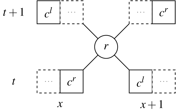
The local rule is the one that transports the right component of the state to the right and the left component of the state to the left. Formally, let us denote by $R$ the CA with local evolution $r$ . Focussing on the next left component of the state at position $x$ and right component of the state at position $x+1$ for time $t+1$ we have the following equation:

	$\displaystyle(c^{l}_{t+1,x},c^{r}_{t+1,x+1})$	$\displaystyle=r(c_{t,x},c_{t,x+1})$		(6)
		$\displaystyle=(c^{l}_{t,x+1},c^{r}_{t,x})$		(7)

$r$ is not a local rule properly speaking because it does not compute the value of a specific cell but two components of two different cells. However, it can be formulated as a local rule with neighbourhood $1$ —i.e. the cell at position $x$ is computed from the previous values of the cells at positions $x-1$ and $x+1$ .

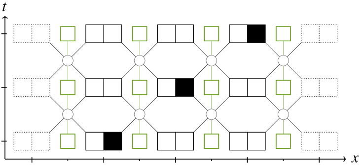
This evolution is illustrated in Fig. 2.

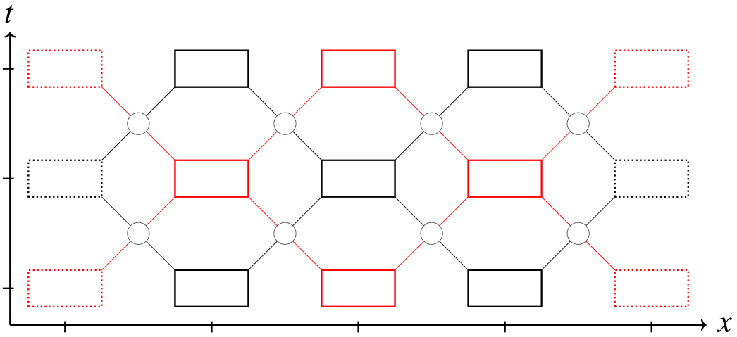
At this point, one can notice that the CA is made of two independent grids (the one for which $x+t$ is even, and the one for which $x+t$ is odd) as shown in Fig. 3. Indeed, since the evolution takes the left component of a state to the left and similarly for the right component, there is no interaction between a cell at position $x$ and one at position $x+1$ at time $t$ . Still, both grids are kept here so that the framework stays the same for later examples.

In this example, $G=\{I\otimes I,\tau\otimes\tau\}$ with $I$ the identity, $\tau(0)=1$ and $\tau(1)=0$ . Changing identically both components of the state is also what is usually done in Physics. Notice that $G$ is abelian ; in Sec. 4, a non-abelian example will be detailed.

Verification of the gauge-invariance.

Having a CA $R$ and the set of gauge transformations $\Gamma$ , the next step is to check whether it is gauge-invariant. Showing that a CA is not gauge-invariant can usually be done in quite a straightforward way by applying different gauge transformations on the different inputs of the local evolution rule (or local unitary in the quantum case).

Example (1).

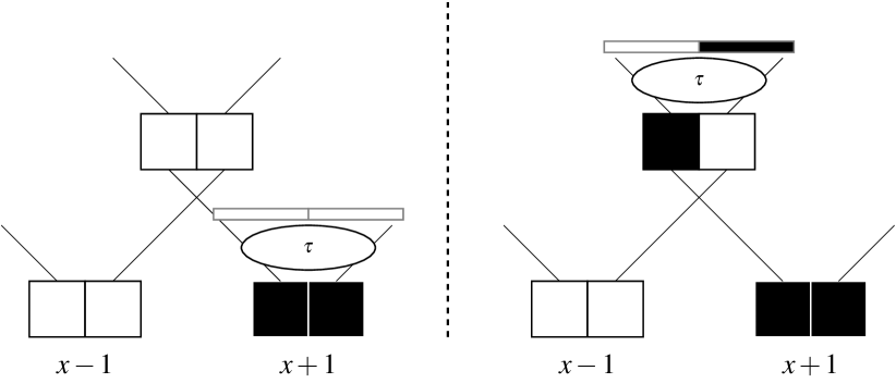
The example is not gauge-invariant. This is illustrated in Fig. 4 where the gauge transformation before the evolution (left side of the figure) cannot be compensated after the evolution (right side of the figure): whatever local gauge transformation is applied after the evolution, the final state on both sides of the figure will never match.

3.2 Introducing the gauge field.

If the CA is not gauge-invariant, then, following the Physics tradition, we seek to extend it into a wider CA, acting over the original field plus a gauge field. This gauge field also changes under a gauge transformation, and it is with respect to this extended gauge transformation that the extended CA will be gauge-invariant.

Positioning.

The first question that arises is the positioning of the gauge field. In the lattice-gauge theory tradition, the usual way to position the gauge field is in-between every two states as shown in Fig. 5.

Example (1).

In this example, we make the standard choice of having the gauge field positioned in between every two-states. Therefore we will denote by $A_{x,x+1}$ the value of the gauge field in between the position $x$ and $x+1$ .

Set of values.

The second question that arises is what set of values $\Lambda$ can the gauge field take? Usually, one seeks to add the least amount of information that will allow for gauge-invariance. Often it turns out that the gauge field keeps track of the difference of gauge between the states that surrounds it—i.e. it is analogous to a parallel transport operator between two separate tangent spaces in a differential manifold.

Example (1).

In this example, we chose $\Lambda=\{I\otimes I,\tau\otimes\tau\}$ . Since there are only two elements in $\Lambda$ , the values of this set can be encoded in a single bit.

This choice is motivated by the fact that the difference of gauge between two neighboring positions can only be one of the elements of $\Lambda$ .

In sec-4, other examples for the set of values of the gauge field will be developed.

Updating the local rule.

Having defined where and what the gauge field is, the third question that arises is: how does it interact with a configuration? More specifically, how does the local rule (or local unitary) depend on the gauge field? Usually the gauge field keeps track of the difference of gauge between neighboring states, and so usually the gauge field is used to cancel this difference.

Example (1).

One choice for the extended local rule is to harmonize the gauges of the inputs before applying the previously defined local rule. To do so, in our example Eq. (6) transforms into:

	$\displaystyle(c^{l}_{t+1,x},c^{r}_{t+1,x+1})$	$\displaystyle=r_{A}(c_{t,x},c_{t,x+1})$		(8)
		$\displaystyle=r\left(A_{x,x+1}\big{(}c_{t,x}\big{)},A^{-1}_{x,x+1}\big{(}c_{t,x+1}\big{)}\right)$		(9)

where $r_{A}$ denote the extended, $A$ -dependant, local rule.

Gauge transformation.

The role of the gauge field at this point is to obtain gauge-invariance. Writing the gauge-invariance condition (5) forces a fourth question: how does the gauge field transform under a gauge transformation? To answer this question, one need to write down the gauge-invariance condition, which puts a constraint over the transformation of the gauge field.

If the gauge field does not change under a gauge transformation, one can easily see that adding the gauge field does not help acquire gauge-invariance, since the information added through the gauge field would not help cancel the effect of gauge transformations. Therefore, the gauge transformations need to be extended to also act upon the gauge field. The set of extended gauge transformations will be denoted $\overline{G}$ .

Example (1).

The action of the gauge transformation, in between position $x$ and $x+1$ , over $A_{x,x+1}$ will be denoted by $g(A_{x,x+1})$ . This choice will help to stay clear of new notations. The gauge-invariance condition (5) puts a constraint which may wholly determine this action. Locally, for the running example with $g_{x},g_{x+1}$ two elements of $G$ , the gauge-invariance condition writes:

\displaystyle r_{g(A)}\circ(g_{x}\otimes g_{x+1})=({Z(g)_{x}}\otimes{Z(g)_{x+1}})\circ r_{A}

(10)

The gauge-invariance condition requires the existence of a CA $Z$ . Here we choose $Z=Id$ (but other choices would have been possible). Thus, Eq. (10) transforms into the following two equations:

\begin{cases}g(A_{x,x+1})^{-1}\circ g_{x}&=g_{x+1}\circ A_{x,x+1}\\ g(A_{x,x+1})\circ g_{x+1}&={g_{x}}\circ A^{-1}_{x,x+1}\end{cases}

(11)

Those two equations are redundant and simplify into:

g(A_{x,x+1})=g_{x}\circ A_{x,x+1}\circ g_{x+1}

(12)

Therefore, from the gauge-invariance condition and through the choice of a $Z$ , the extension of gauge transformations to the gauge field is fully determined. Here they are expressed in a gauge-field centric way, however let us express them equivalently in a way that is centered on $x$ .

Indeed, after this extension, the local gauge transformation group $G$ is extended into a subgroup $\overline{G}$ of the bijection over $\Lambda\otimes\Sigma\otimes\Lambda$ . Then for any $\overline{g}\in\overline{G}$ , we define $g\in G$ such that for any $A_{0},c,A_{1}\in\Lambda\otimes\Sigma\otimes\Lambda$ :

\overline{g}\big{(}A_{0},\;c,\;A_{1})=\Big{(}A_{0}\circ g,\;g(c),\;g\circ A_{1}\Big{)}

(13)

The application of this local gauge transformation is illustrated in Fig. 6.

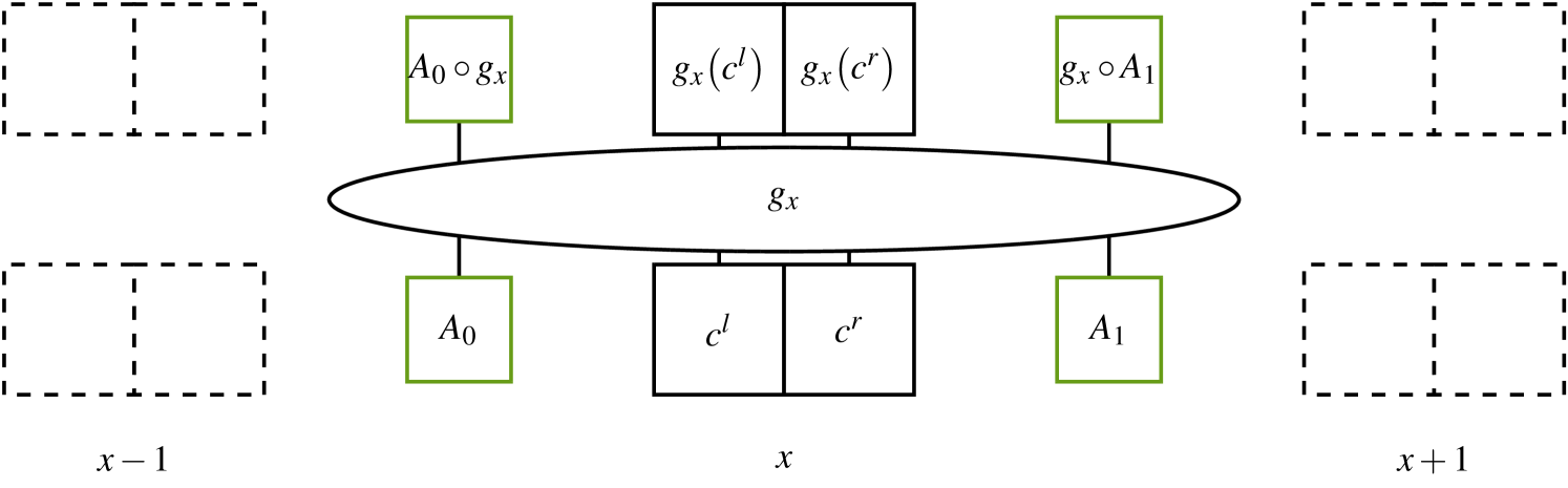
The extended local gauge transformations no longer have disjoint supports, but they do commute with one another:

g_{x+1}\circ g_{x}(A_{x,x+1})=g_{x+1}\circ A\circ g_{x}=g_{x}\circ g_{x+1}(A_{x,x+1})

for any $A_{x,x+1}$ in $\Lambda$ . Therefore, the set of extended gauge transformations $\Gamma$ , over a full configuration and its associated gauge field, can be defined through definition-7.

After this step, the CA is gauge-invariant through the use of an external gauge field and an extended gauge transformation.

3.3 Dynamics of the gauge field.

The last step of this procedure is to transform the external gauge field into an internal state of the CA which will evolve through a local rule. This leads to the fifth and final question: what is the dynamics of the gauge field? The choice of dynamics is constrained by the fact that the complete dynamics should be gauge-invariant—i.e. verify condition (5) for $\overline{G}$ .

Example (1).

In our running example a simple gauge-invariant dynamics for the gauge field, is to choose the identity. Eq. (8) thus transforms into:

	$\displaystyle\left(c^{l}_{t+1,x},A_{t+1,x,x+1},c^{r}_{t+1,x+1}\right)$	$\displaystyle=r\left(c_{t,x},A_{t,x,x+1},c_{t,x+1}\right)$		(14)
		$\displaystyle=\left({A_{t,x,x+1}}\big{(}c^{l}_{t,x+1}\big{)},\;A_{t,x,x+1},\;{A_{t,x,x+1}}\big{(}c^{r}_{t,x}\big{)}\right)$		(15)

The identity is indeed gauge-invariant with respect to $\Gamma$ and $Z$ in this example. This is due to the fact that $Z$ is the identity and as such, Eq. (5) is a simple commutation relation which is trivially true for the identity.

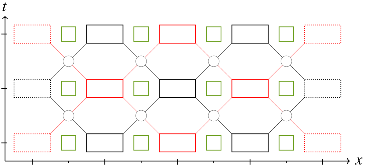
This complete evolution is represented graphically in Fig. 7.

4 Examples of reversible and quantum constructions

The procedure helps designing new CA that implement gauge-invariance. In this section, examples both in classical and quantum settings will be developed. Every example presented here have the same space-time layout as that of Fig. 7. This choice is made for simplicity and clarity, but there is no claim of generality. Although it is known that PQCA are intrinsically universal arrighi2012partitioned , it could be that they are not the most general setting in which to define gauge-invariant CA.

For all of these examples, the local evolution $Z$ of the gauge transformations will be taken to be the identity. Then again, this is only a choice.

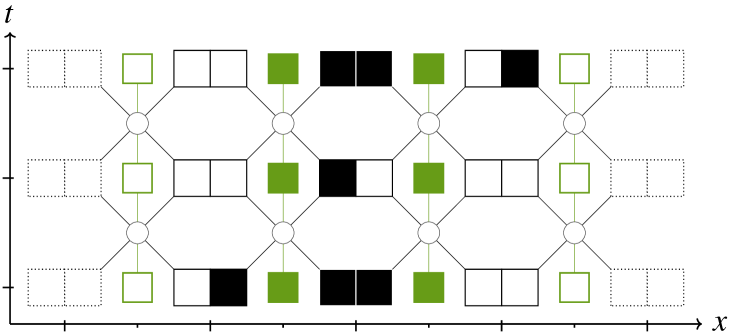
Example (1).

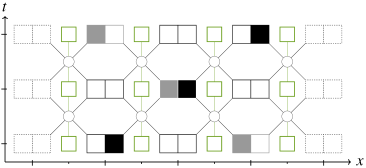
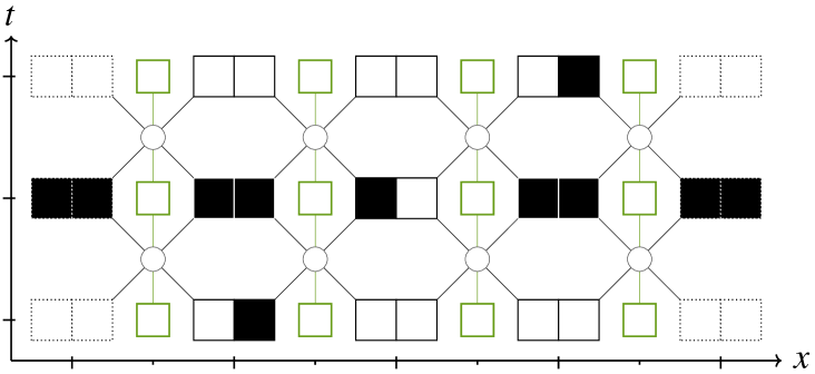
This example has been developed extensively in the previous sections. Fig. 8 shows three space-time diagrams implementing the gauge-invariant rule given in Eq.(14). An empty state for the gauge field (in green) represents the identity while a filled state represents $\tau\otimes\tau$ .

Sub-figure LABEL:sub@subfig:rcaa1 has its gauge field set to the identity, therefore coincides with $R$ , with a ”particle” going right. Sub-figure LABEL:sub@subfig:rcaa2 features the same physics (a particle going right) but with a gauge transformation initially applied at the central position. This is therefore understood as an equivalent situation, expressed differently. Indeed, if a gauge transformation is later applied at the central position, the final configuration yields back that of sub-figure LABEL:sub@subfig:rcaa1. Finally, Sub-figure LABEL:sub@subfig:rcaa3 starts with a similar configuration as sub-figure LABEL:sub@subfig:rcaa1 but with one difference in the gauge field, that does not come from having applied a gauge transformation. Both diagrams end up very different. This last sub-figure shows that new dynamical behaviours arise, which could not have been witnessed without a gauge field.

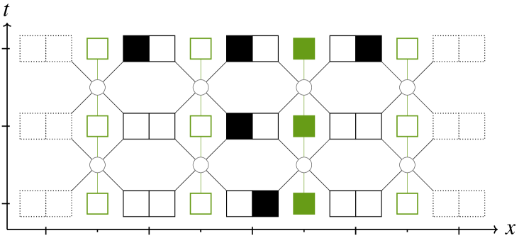
Example (2).

In Physics, a distinction is often made between abelian and non-abelian gauge theories. The abelian gauge theory accounts for quantum electrodynamics (QED) while non-abelian gauge theory accounts, for example, for quantum chromodynamics (QCD).

It is easy to extend example (1) to become non-abelian by extending the alphabet $\Sigma$ to $\{1,...,N\}^{2}$ for $N>2$ . $G$ (the local gauge transformation restricted to the states $\Sigma$ ) is again a set of permutations that change both components of the state in the same way. In fact we take all of them:

G=\{\sigma\otimes\sigma\;|\;\sigma\in S(N)\}

with $S(N)$ the set of permutations over $N$ elements. We can then define the gauge field to again be $\Lambda=G$ ; the extended local gauge transformations $\overline{G}$ through Eq. (13) and the set of gauge transformations $\Gamma$ through definition-7. Two local gauge transformations $g_{x}$ and $g_{x+1}$ do commute for the same reason as in the abelian case, thus $\Gamma$ is well defined.

Using those definitions, the local rule defined in Eq. (14) is already gauge-invariant. This can be checked in a straightforward manner through the exact same procedure as the abelian case.

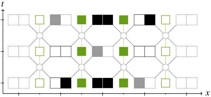
Fig. 9 gives two space-time diagrams of a non-abelian gauge-invariant CA with $N=3$ —i.e. $|\Sigma|=9$ and $|G|=3!=6$ . An empty state for the gauge field represents the identity and a filled state represents $\tau\otimes\tau$ where $\tau$ is the permutation between black and white, leaving the gray untouched. Only those two state are represented here to keep the figure readable, even though there are more transformations available.

Sub-figure LABEL:sub@subfig:rcana1 features an example of two ”particles” crossing. Sub-figure LABEL:sub@subfig:rcana2 represents just the same scenario, only with a gauge transformation $\tau\otimes\tau$ has been applied in the middle.

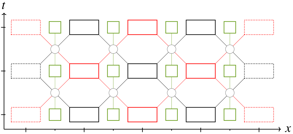
Example (3).

Now switching from the classical to the quantum setting, the same gauging procedure has been applied to obtain a gauge-invariant QCA Arrighi2020 , in the abelian case. This example will not be treated in detail, only the definition of the model and the reason for it being gauge-invariant will be given here.

The classical configuration are obtained again from alphabet $\Sigma=\{0,1\}^{2}$ . These two boolean numbers code the presence, or the absence of two fermions. The pseudo-spin of the fermion is encoded by the choice of the component, i.e. $01$ is the left-moving spin, $10$ is the right-moving spin. There can be two fermions of opposite spin, which is the state $11$ , but there cannot be two fermions of the same spin, by the Pauli exclusion principle. This is sometimes referred to as the occupation number representation. The gauge field can be seen as a counter of particles.

Evolution rule.

$r$ is now a unitary matrix that acts on $\mathcal{H}_{\Sigma}\otimes\mathcal{H}_{\Lambda}\otimes\mathcal{H}_{\Sigma}$

r=\begin{pmatrix}I&0&0&0\\ 0&-isI&cV&0\\ 0&cV^{\dagger}&-isI&0\\ 0&0&0&-I\end{pmatrix}e^{\frac{i}{2}\epsilon^{2}g^{2}L^{2}}

(16)

with $g$ a parameter called the charge, $\epsilon$ the distance between two points in space, $I$ the identity, $s$ and $c$ stands for $sin(m\epsilon)$ and $cos(m\epsilon$ ) respectively where $m$ is the mass, and for $l\in\mathbb{Z}$ :

$V\ket{l}=\ket{l-1}$
$L\ket{l}=l\ket{l}$ .

This evolution rule defines the dynamics directly for both the fermions and the gauge field. When $g=0$ this dynamics is just a non-interacting, multi-particle version of the Dirac quantum walk. If, furthermore, the mass is zero, the fermions do not change direction. The operator $V$ and its conjugate transpose $V^{\dagger}$ allows for the gauge field to act as a counter of fermions that go through the link between two nodes. The exponential term is given here so as to be complete. It is the one which creates the interaction between the gauge field and the fermions. It will have no impact in the proof of gauge-invariance.

The minus sign of the bottom-right entry of the matrix is needed in the qubit representation of two fermions crossing past each other. For the same reason, right before each new cell is formed, the following gate is applied on the incoming components.

S=\begin{pmatrix}\;1\;&\;0\;&\;0\;&\;0\;\\ 0&1&0&0\\ 0&0&1&0\\ 0&0&0&-1\\ \end{pmatrix}

(17)

Gauge transformations.

For $x$ a position, the local gauge transformation $g_{x}$ acts on the fermionic field at position $x$ and on the gauge field in positions $(x-1,x)$ and $(x,x+1)$ which is reminiscent of the classical case. For $\varphi\in\mathbb{R}$ , we define

	$\displaystyle R_{\varphi}:$	$\displaystyle\ket{0}\mapsto\ket{0}$		(18)
		$\displaystyle\ket{1}\mapsto e^{i\varphi}\ket{1}$		(19)

which is a $U(1)$ gauge transformation, and for $l\in\mathbb{Z}$ :

T_{\varphi}\ket{l}=e^{il\varphi}\ket{l}.

(20)

Then the group $G$ is defined using $R_{\varphi}$ and $T_{\varphi}$ for any $\varphi$ in $\mathbb{R}$ , where $R_{\varphi}$ is applied on each component of a state in $\Sigma$ and $T_{\varphi}$ is applied to the gauge field:

G=\Big{\{}T_{\varphi}\otimes\big{(}R_{\varphi}\otimes R_{\varphi}\big{)}\otimes T_{-\varphi}\;|\;\varphi\in\mathbb{R}\Big{\}}

(21)

The local gauge transformation at positions $x$ and $y$ commute, so the gauge transformation set $\Gamma$ can again be defined through definition-7 as the set of operators that apply, locally, any local gauge transformation.

Gauge-invariance.

This model is gauge-invariant with $Z$ as the identity. In order to prove it let us focus on the input $\ket{mln}$ of a gate. When applying a gauge transformation $g_{\varphi}$ , this input state will trigger a phase gain $\mathcal{V}(x,m-l,n+l)$ :

	$\displaystyle m\varphi(x)+l\big{(}\varphi(x+1)-\varphi(x)\big{)}+n\varphi(x+1)$		(22)
	$\displaystyle=(m-l)\varphi(x)+(n+l)\varphi(x+1).$		(23)

However, the numbers $(m-l,n+l)$ are invariants of $r$ , as it takes $\ket{mln}$ into a superposition of the form:

\sum_{i\in\{-1,0,1\}}\alpha_{i}\ket{m-i,l-i,n+i}.

(24)

It follows that the phase gain will be the same whether the gauge transformation is applied before or after the evolution and thus, the evolution commutes with the gauge transformations. Hence, the QCA is gauge-invariant under $\gamma$ and for $Z$ being the identity.

Physical model.

This QCA is quite specific because it was conceived so that it provides a discrete space-time formulation of one-dimensional quantum electrodynamics, which is one of the four fundamental interactions in Physics Arrighi2020 . The continuous limit for this specific model has not been formally derived, however this limit has been done in the free case both for continuous time di2020quantum ; Manighalam2021ContinuousTL and the same method could potentially work in this case.

5 Degrees of freedom induced by gauge-invariance

5.1 Equivalence of theories

Given a set of gauge transformations $\Gamma$ , multiple CA may lead to equivalent dynamics up to $\Gamma$ :

Definition 9 (Equivalence of gauge-invariant CA).

Let $T$ be a gauge-invariant CA with respect to a given $\Gamma$ and $Z$ . $T$ is simulated by a CA $T^{\prime}$ if and only if for each element $c$ of $\mathcal{C}$ (or $\mathcal{H}$ in the quantum case) there exists $\gamma,\gamma^{\prime}\in\Gamma$ such that $(\gamma\circ T)(c)=(T^{\prime}\circ\gamma^{\prime})(c)$ . They are equivalent if both simulate each other. Equivalence will be denoted $T\equiv T^{\prime}$ .

In practice, $T$ is gauge-invariant with respect to a specific $\Gamma$ and $Z$ . Adding a constraint on $Z$ , one may characterize the equivalence of two CA using different quantifiers and constraints which may be useful for some specific problems.

Proposition 1 (Characterization of equivalence for gauge-invariant CA).

Let $T$ be a gauge-invariant CA with respect to $\Gamma$ and $Z$ and $T^{\prime}$ another CA over the same alphabet as $T$ . If $Z$ is reversible and $T^{\prime}$ is gauge-invariant with respect to $\Gamma$ and $Z$ , then these three statements are equivalent:

1.

$T$ is simulated by $T^{\prime}$ .
2.

$\forall c,\exists\gamma\in\Gamma$ such that $T(c)=T^{\prime}\circ\gamma(c)$ .
3.

$\forall c,\forall\gamma\in\Gamma$ , $\exists\gamma^{\prime}\in\Gamma$ such that $\gamma\circ T(c)=T^{\prime}\circ\gamma^{\prime}(c)$ .

Proof.

We shall prove the equivalence through three implications. The proof is given in the classical setting, but carries through to the quantum case where $c$ takes its value in $\mathcal{H}$ instead of $\mathcal{C}$ .

•

Suppose (1), then for $c$ a configuration, we have $\gamma,\gamma^{\prime}\in\Gamma$ such that $(\gamma\circ T)(c)=(T^{\prime}\circ\gamma^{\prime})(c)$ . But since $\Gamma$ is a group, it implies that $T(c)=(\gamma^{-1}\circ T^{\prime}\circ\gamma^{\prime})(c)$ . And since $Z$ is reversible, we obtain $T(c)=(T^{\prime}\circ Z^{-1}(\gamma^{-1})\circ\gamma^{\prime})(c)$ . However, $Z^{-1}(\gamma^{-1})\circ\gamma^{\prime}$ is an element of $\Gamma$ therefore we have proven that (1) implies (2).
•

Suppose (2), let $c$ be a configuration and take $\gamma\in\Gamma$ such that $T(c)=(T^{\prime}\circ\gamma)(c)$ . Since $\Gamma$ is a group, for any $\gamma_{1}\in\Gamma$ there exists $\gamma_{3}\in\Gamma$ such that $\gamma=\gamma_{3}\circ\gamma_{1}$ . Therefore, from gauge-invariance of $T^{\prime}$ , $T(c)=(Z(\gamma_{3})\circ T^{\prime}\circ\gamma_{1})(c)$ which is equivalent to $(Z(\gamma_{3})^{-1}\circ T)(c)=(T\circ\gamma_{1})(c)$ because $G$ is a group. And writing $\gamma_{2}=Z(\gamma_{3})^{-1}$ which is in $\Gamma$ , we conclude that (2) implies (3).
•

The fact that (3) implies (1) is immediate because (3) is a generalization of (1): both statements differ only by the quantifier before $\gamma$ . If for any $\gamma$ the property is true, then it is also true for one specific $\gamma$ .

Example (1).

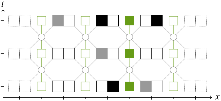
Fig. 10 shows two diagrams of equivalent CA. The local rule $r$ driving the evolution in sub-figure LABEL:sub@subfig:equiv1 is the one given in Eq.(14) for the abelian example whilst the local rule driving the evolution of sub-figure LABEL:sub@subfig:equiv2 is $r^{\prime}=\gamma\circ r$ where $\gamma$ is the gauge transformation that swaps black and white everywhere (note that this does not impact the gauge field because the transformation on each side of it cancel out).

5.2 Gauge-fixing and gauge-constraining

Gauge-invariance states that there is a degree of freedom in both the dynamics—equivalence of CA—and the set of possible states. Gauge-fixing means choosing, amongst the many possible dynamics. Gauge-constraining, on the other hand, deals with the removal of the degrees of freedom, e.g. via the choice of a canonical representative element for each class of gauge equivalent configurations.

Gauge-fixing.

With equivalence of CA, one can use many different representations for the same evolution model: two equivalent CA will model the same dynamics up to a gauge transformation. Therefore, there is a degree of freedom in choosing a specific CA as a model for a specific dynamics. Choosing this degree of freedom is called gauge-fixing.

In other words, the explicit evolution scheme is undetermined because of the gauge-invariance: if a configuration $c$ at times $t$ evolves into a configuration $c^{\prime}$ , it is the same as if it evolved into $\gamma(c^{\prime})$ for $\gamma$ a gauge transformation. Gauge-fixing is the choice of an explicit evolution scheme.

Gauge-constraining.

The redundancy induced by gauge-invariance is somewhat problematic, because it is there in the state space, when really it should not be observable. In other words, a gauge transformation should not alter the observation. In quantum mechanics, for a system described by a density matrix $\rho$ , what is being measured for $\mathcal{O}$ an observable, is the expected value:

Tr(\mathcal{O}\rho).

A gauge transformation $\gamma$ is a unitary that will act on a density matrix as follows :

\rho\mapsto\gamma\rho\gamma^{\dagger}

with $\gamma^{\dagger}$ being the conjugate transpose of $\gamma$ .

One may wish to restrict the states, or observables, to being physical. That is to say for any gauge transformation $\gamma$ , the equality $Tr(\mathcal{O}\,\rho)=Tr\big{(}\mathcal{O}\gamma\rho\gamma^{\dagger}\big{)}$ should hold. There are two ways to do so, one is to restrict the set of allowed observables to those which commute with the gauge transformations. Indeed, by the cyclic property of the trace, the action of $\gamma$ and $\gamma^{\dagger}$ will then cancel out.

Another way is to allow any set of observables but to restrict the states to those which commute with gauge transformations—i.e. $[\gamma,\rho]=0$ for any gauge transformation $\gamma$ . This is called gauge-constraining. Again, this would lead to $\gamma$ and $\gamma^{\dagger}$ cancelling out.

Gauge-constraining is frequently used in Physics, but still remains to be formulated for classical CA.

6 Conclusion

Summary.

The paper followed a constructive approach to gauge-invariance in Cellular Automata (CA). Formal definitions of CA, gauge transformations and gauge-invariance were given. For $R$ a CA and $\Gamma$ a set of gauge transformations, it was shown how to obtain a gauge-invariant CA $T$ through the introduction of a gauge-field, whilst keeping $R$ as a sub-case. The extension of $R$ into $T$ is called gauging procedure and comes from Physics. Three examples of gauge-invariant CA were then given, for abelian and non-abelian gauge transformation in classical CA, and for abelian gauge transformations in a QCA. Because of the redundancy inherent to gauge-invariance, CA implementing a gauge-invariance with respect to the same set of gauge transformations can have the same dynamics up to gauge transformations, which means those two theories are equivalent. The equivalence of CA was defined and characterized. Finally, gauge-fixing and gauge-constraining were introduced as ways for choosing or removing the degrees of freedom induced by gauge-invariance.

Related works.

A number of discrete counterparts to Physics symmetries have been reformulated in terms of CA, including reversibility, Lorentz-covariance arrighi2014discrete and conservations laws and invariants formenti2011hierarchy . To our knowledge the closest work is the colour-blind CA construction salo2013 which implements a global colour symmetry without porting it to the local scale. However gauge symmetries have been implemented in the one-particle sector of Quantum CA, a.k.a for Quantum Walks arnaultdebbasch2016quantum ; arnault2017discrete ; cedzich2019quantum . One of the authors had followed a similar procedure in order to introduce the electromagnetic gauge field di2014quantum ; marquez2018electromagnetic , and that of the weak and strong interactions arnault2016quantum ; di2016quantum . This again was done in the very fabric of the Quantum Walk and the associated symmetry was therefore an intrinsic property of the Quantum Walk. But the gauge field would remain continuous, and seen as an external field. Recently, this symmetry has been studied in the classical CA for both abelian and non-abelian gauge-invariance arrighi2018gauge ; arrighi2019non and for a QCA as well Arrighi2020 .

There are, of course, numerous other approaches to space-discretized gauge theories, the main ones being Lattice Gauge Theory banuls2017efficient ; emonts2020gauss ; kaplan2020gauss ; rothe2012lattice and the Quantum Link Model chandrasekharan1997quantum , which were phrased in terms of Quantum Computation–friendly terms through Tensor Networks rico2014tensor ; zohar2018combining and can be linked in a unified framework silvi2014 . The tensor network representation is based on the locality of the Hamiltonian evolution, the system is not described in terms of large vectors, but with local tensors and boundary constraints, allowing for a more efficient description. Changing the parameters of the tensor using variational optimization techniques—e.g. gradient descent—over the expected energy $\bra{\psi}H\ket{\psi}$ allows to recover the ground state which describes the low-energy Physics of the system ercolessi2018phase ; felser2020two ; magnifico2020real ; magnifico2021lattice ; notarnicola2015discrete . Discretized gauge-theories have also arisen from other horizons, such as Ising models silvi2014 ; wegner1971 . With the recent progress in quantum hardware—e.g. trapped ions, Rydberg atoms, quantum superconducting—quantum simulations can also be directly implemented on quantum technologies banuls2020simulating ; klco20202 .

All of these approaches, however, begin with a well-known continuous gauge theory which is then space-discretized—time is usually kept continuous. An interesting attempt to quantum discretize gauge theories in discrete time, on a general simplicial complex can be found in kornyak2009discrete .

At the time of the writing, some theoretical questions about gauge-invariant cellular automata remained open. Is it always possible to make a CA gauge-invariant under any groups of gauge transformation? How do this model relate to color-blind cellular automata salo2013 ? These two questions have since then been answered by two of the authors arrighi_et_al:LIPIcs.MFCS.2021.9 .

Perspectives.

The hereby developed methodology has already been applied to Quantum CA (QCA) Arrighi2020 with abelian gauge symmetry, so as to obtain the Schwinger model for quantum electrodynamics. We believe it can be further extended to non-abelian gauge-invariance in order to have, for example, a discrete counterpart to quantum chromodynamics, and to 2 or 3 dimensions in space so as to expand the possible dynamics. Such discretized theories may be of interest in Physics especially in non-perturbative theories strocchi2013introduction , but they may also represent practical assets as quantum simulation algorithms, i.e. numerical schemes that run on Quantum Computers to efficiently simulate interacting fundamental particles theories—a task which would take a very long time on classical computers.

Another perspective lies in error-correction. Taking the set of gauge transformations to be the set of errors, we expect that gauge-invariance provides a way to obtain a dynamics that would be error-free. Applied in the context of CA, this would correspond to error-correction in spatially distributed systems.

Acknowledgements.

NE would like to thank Simone Montangero and Giuseppe Magnifico for helpful discussions. GDM acknowledges the invitational Fellowships for Research in Japan supported by Japan Society for the Promotion of Science (JSPS), Bridge Program (ID: BR190201). This publication was made possible through the support of the ID# 61466 grant from the John Templeton Foundation, as part of the “The Quantum Information Structure of Spacetime (QISS)” Project (qiss.fr). The opinions expressed in this publication are those of the author(s) and do not necessarily reflect the views of the John Templeton Foundation.

References

(1) Arnault, P.: Discrete-time quantum walks and gauge theories. arXiv preprint arXiv:1710.11123 (2017)
(2) Arnault, P., Debbasch, F.: Quantum walks and discrete gauge theories. Physical Review A 93(5), 052301 (2016)
(3) Arnault, P., Di Molfetta, G., Brachet, M., Debbasch, F.: Quantum walks and non-abelian discrete gauge theory. Physical Review A 94(1), 012335 (2016)
(4) Arrighi, P.: An overview of quantum cellular automata. Natural Computing 18(4), 885–899 (2019)
(5) Arrighi, P., Bény, C., Farrelly, T.: A quantum cellular automaton for one-dimensional QED. Quantum Information Processing 19 (2020). DOI 10.1007/s11128-019-2555-4
(6) Arrighi, P., Costes, M., Eon, N.: Universal Gauge-Invariant Cellular Automata. In: F. Bonchi, S.J. Puglisi (eds.) 46th International Symposium on Mathematical Foundations of Computer Science (MFCS 2021), Leibniz International Proceedings in Informatics (LIPIcs), vol. 202, pp. 9:1–9:14. Schloss Dagstuhl – Leibniz-Zentrum für Informatik, Dagstuhl, Germany (2021). DOI 10.4230/LIPIcs.MFCS.2021.9. URL https://drops.dagstuhl.de/opus/volltexte/2021/14449
(7) Arrighi, P., Di Molfetta, G., Eon, N.: A gauge-invariant reversible cellular automaton. In: International Workshop on Cellular Automata and Discrete Complex Systems, pp. 1–12. Springer (2018)
(8) Arrighi, P., Di Molfetta, G., Eon, N.: Non-abelian gauge-invariant cellular automata. In: International Conference on Theory and Practice of Natural Computing, pp. 211–221. Springer (2019)
(9) Arrighi, P., Facchini, S., Forets, M.: Discrete lorentz covariance for quantum walks and quantum cellular automata. New Journal of Physics 16(9), 093007 (2014)
(10) Arrighi, P., Grattage, J.: Partitioned quantum cellular automata are intrinsically universal. Natural Computing 11(1), 13–22 (2012)
(11) Banuls, M.C., Blatt, R., Catani, J., Celi, A., Cirac, J.I., Dalmonte, M., Fallani, L., Jansen, K., Lewenstein, M., Montangero, S., et al.: Simulating lattice gauge theories within quantum technologies. The European physical journal D 74(8), 1–42 (2020)
(12) Bañuls, M.C., Cichy, K., Cirac, J.I., Jansen, K., Kühn, S.: Efficient basis formulation for (1+ 1)-dimensional su (2) lattice gauge theory: Spectral calculations with matrix product states. Physical Review X 7(4), 041046 (2017)
(13) Cedzich, C., Geib, T., Werner, A., Werner, R.: Quantum walks in external gauge fields. Journal of Mathematical Physics 60(1), 012107 (2019)
(14) Chandrasekharan, S., Wiese, U.J.: Quantum link models: A discrete approach to gauge theories. Nuclear Physics B 492(1-2), 455–471 (1997)
(15) Di Molfetta, G., Arrighi, P.: A quantum walk with both a continuous-time limit and a continuous-spacetime limit. Quantum Information Processing 19(2), 47 (2020)
(16) Di Molfetta, G., Brachet, M., Debbasch, F.: Quantum walks in artificial electric and gravitational fields. Physica A: Statistical Mechanics and its Applications 397, 157–168 (2014)
(17) Di Molfetta, G., Pérez, A.: Quantum walks as simulators of neutrino oscillations in a vacuum and matter. New Journal of Physics 18(10), 103038 (2016)
(18) Emonts, P., Zohar, E.: Gauss law, minimal coupling and fermionic peps for lattice gauge theories. SciPost Physics 12 (2020)
(19) Ercolessi, E., Facchi, P., Magnifico, G., Pascazio, S., Pepe, F.V.: Phase transitions in z n gauge models: Towards quantum simulations of the schwinger-weyl qed. Physical Review D 98(7), 074503 (2018)
(20) Felser, T., Silvi, P., Collura, M., Montangero, S.: Two-dimensional quantum-link lattice quantum electrodynamics at finite density. Physical Review X 10(4), 041040 (2020)
(21) Formenti, E., Kari, J., Taati, S.: On the hierarchy of conservation laws in a cellular automaton. Natural Computing 10(4), 1275–1294 (2011)
(22) Georgescu, I., Ashhab, S., Nori, F.: Quantum simulation. Reviews of Modern Physics 86(1), 153 (2014)
(23) Harao, M., Noguchi, S.: Fault tolerant cellular automata. Journal of computer and system sciences 11(2), 171–185 (1975)
(24) Hastings, W.K.: Monte carlo sampling methods using markov chains and their applications. Biometrika 57(1), 97–109 (1970)
(25) Kaplan, D.B., Stryker, J.R.: Gauss’s law, duality, and the hamiltonian formulation of u (1) lattice gauge theory. Physical Review D 102(9), 094515 (2020)
(26) Kitaev, A.Y.: Fault-tolerant quantum computation by anyons. Annals of Physics 303(1), 2–30 (2003)
(27) Klco, N., Savage, M.J., Stryker, J.R.: Su (2) non-abelian gauge field theory in one dimension on digital quantum computers. Physical Review D 101(7), 074512 (2020)
(28) Kornyak, V.V.: Discrete dynamics: gauge invariance and quantization. In: International Workshop on Computer Algebra in Scientific Computing, pp. 180–194. Springer (2009)
(29) Magnifico, G., Dalmonte, M., Facchi, P., Pascazio, S., Pepe, F.V., Ercolessi, E.: Real time dynamics and confinement in the $\mathbb{Z}_{n}$ schwinger-weyl lattice model for 1+ 1 qed. Quantum 4, 281 (2020)
(30) Magnifico, G., Felser, T., Silvi, P., Montangero, S.: Lattice quantum electrodynamics in (3+ 1)-dimensions at finite density with tensor networks. Nature Communications 12(1), 1–13 (2021)
(31) Manighalam, M., Molfetta, G.D.: Continuous time limit of the dtqw in 2d+1 and plasticity. Quantum Inf. Process. 20, 76 (2021)
(32) Márquez-Martín, I., Arnault, P., Di Molfetta, G., Pérez, A.: Electromagnetic lattice gauge invariance in two-dimensional discrete-time quantum walks. Physical Review A 98(3), 032333 (2018)
(33) Nayak, C., Simon, S.H., Stern, A., Freedman, M., Sarma, S.D.: Non-abelian anyons and topological quantum computation. Reviews of Modern Physics 80(3), 1083 (2008)
(34) Notarnicola, S., Collura, M., Montangero, S.: Real-time-dynamics quantum simulation of (1+ 1)-dimensional lattice qed with rydberg atoms. Physical Review Research 2(1), 013288 (2020)
(35) Notarnicola, S., Ercolessi, E., Facchi, P., Marmo, G., Pascazio, S., Pepe, F.V.: Discrete abelian gauge theories for quantum simulations of qed. Journal of Physics A: Mathematical and Theoretical 48(30), 30FT01 (2015)
(36) Quigg, C.: Gauge theories of the strong, weak, and electromagnetic interactions. Princeton University Press (2013)
(37) Rico, E., Pichler, T., Dalmonte, M., Zoller, P., Montangero, S.: Tensor networks for lattice gauge theories and atomic quantum simulation. Physical Review Letters 112(20), 201601 (2014)
(38) Rothe, H.J.: Lattice gauge theories: an introduction. World Scientific Publishing Company (2012)
(39) Salo, V., Törmä, I.: Color blind cellular automata. Lecture Notes in Computer Science p. 139–154 (2013)
(40) Schumacher, B., Werner, R.F.: Reversible quantum cellular automata. arXiv preprint quant-ph/0405174 (2004)
(41) Silvi, P., Rico, E., Calarco, T., Montangero, S.: Lattice gauge tensor networks. New Journal of Physics 16(10), 103015 (2014). DOI 10.1088/1367-2630/16/10/103015. URL http://dx.doi.org/10.1088/1367-2630/16/10/103015
(42) Strocchi, F.: An introduction to non-perturbative foundations of quantum field theory, vol. 158. Oxford University Press (2013)
(43) Toom, A.: Cellular automata with errors: Problems for students of probability. Topics in Contemporary Probability and Its Applications pp. 117–157 (1995)
(44) Wegner, F.J.: Duality in generalized ising models and phase transitions without local order parameters. Journal of Mathematical Physics 12(10), 2259–2272 (1971). DOI 10.1063/1.1665530. URL http://dx.doi.org/10.1063/1.1665530
(45) Zohar, E., Cirac, J.I.: Combining tensor networks with monte carlo methods for lattice gauge theories. Physical Review D 97(3), 034510 (2018)