Gauge invariant input to neural network for path optimization method

The gauge action is Wilson’s plaquette action Wilson (1974) given by

where $n$ represents the lattice site, and $\beta=1/(ga)^{2}$ is an overall constant consisting of the gauge coupling constant $g$ and the lattice spacing $a$. $P$ ($P^{-1}$) is the plaquette (its inverse). The definition is

where $\hat{\mu}$ is a unit vector in $\mu$-direction and $U_{n,\mu}$ with $\mu=1,2$ are the $U(1)$ link variables. We impose a periodic boundary condition in each direction.

In addition to the plaquette, we measure expectation values of the topological charge $Q$ defined on the lattice,

In the continuum limit, $Q$ recovers the continuum form $Q=(1/4\pi)\int d^{2}x\,\epsilon^{\mu\nu}F_{\mu\nu}(x)$.

The analytic result of this theory has been obtained Wiese (1989); Rusakov (1990); Bonati and Rossi (2019). The partition function $Z$ is represented through the modified Bessel function $I_{n}(\beta)$,

where $V=N_{1}N_{2}$ is the volume factor with $N_{\mu}$ being the lattice size in $\mu$-direction. Since $I_{n}(\beta)$ is well-defined for all complex values of $\beta$, the analytic solution is available over the whole domain of $\beta$.

The path optimization method utilizes complexified dynamical variables to tame the sign problem. In the case of the $U(1)$ gauge theory, the plaquette and the link variable are extended as

where ${\cal A}_{\mu}\in\mathbb{C}$. The modification of the integral path is represented by $y_{n}\in\mathbb{R}$, originated from the imaginary part of ${\cal A}_{\mu}$, which is evaluated by a neural network consisting of the input, a single hidden, and the output layers, as follows. The neural network is a mathematical model inspired by a brain, which is often used for the machine learning McCulloch and Pitts (1943); Rosenblatt (1958); Hebb (2002); Hinton and Salakhutdinov (2006). A sufficient number of the hidden layer units with a non-linear function called an activation function reproduce any continuous function, as proven by the universal approximation theorem Cybenko (1989); Hornik (1991). The variables in the hidden layer nodes ($h_{j}$) and the output ($y_{n}$) are set as

where $i,j=1,\cdots,2\times n_{\mathrm{deg}}$ with the number of the degree of freedom $n_{\mathrm{deg}}$ and $w$, $b$ and $\omega$ are parameters of the neural network. An activation function $F$ defines a relation of data between two layers, the input and hidden layers as well as the hidden and output layers. The activation function is taken to be a tangent hyperbolic function in this work. Our choice of the input $t=\{t_{i}\}$ is the plaquette or the link variable.

We compare (i) with (ii) in terms of the efficiency of the neural network. A schematic picture of our neural network with the plaquette input is given in Fig. 1.

The expectation value of a complexified observable ${\mathcal{O}}$ is calculated by

where $\mathcal{C}$ is the integration path that specifies the complexified link variables $\mathcal{U}=\mathcal{U}(U)$ and the Jacobian $J(\mathcal{U}(U))=\mathrm{det}(\partial\mathcal{U}/\partial U)$. $\theta$ is the phase of $J\,e^{-S_{\rm G}}=e^{i\theta}|J\,e^{-S_{\rm G}}|$. $\langle\cdots\rangle_{\mathrm{pq}}$ denotes the expectation value with the phase quenched Boltzmann weight. In contrast to the naive reweighting, Eq. (12) is evaluated on the modified integration path where the sign problem is maximally weakened by the machine learning without change of the expectation value guaranteed by Cauchy’s theorem. This is the advantage of the path optimization method.

The cost function controls optimization through the neural network. We apply the following cost function ${\cal F}$ to minimize the sign problem,

We evaluate it by the exponential moving average (EMA) as in Ref. Kashiwa and Mori (2020). Using this cost function (13), the neural network finds the best path that enhances $e^{i\theta(t)}$ as much as possible.

We evaluate performance of the POM for $\beta=0.0+(0.25$–$2.25)i$. The sign problem is originated from the imaginary part of $\beta$. We generate gauge configurations by the Hybrid Monte-Carlo algorithm in the POM. The total number of configurations is $50000$. Statistical errors are estimated by the Jackknife method with the bin size of $250$. The neural network utilizes ADADELTA optimizer Zeiler (2012) combined with the Xavier initialization Glorot and Bengio (2010). The parameters in Eqs.(8) and (9) are optimized during learning. The flow chart is displayed in Ref. Kashiwa and Mori (2020). We set the learning rate to 1 and the decay constant 0.95, combined with the batch size of 10. The number of units in the input layer reflects our choice of $t$ in Eqs. (10), (11) as

where $n_{\mathrm{deg}}^{\rm link}=2N_{1}N_{2}$ and $n_{\mathrm{deg}}^{\rm plaq}=N_{1}N_{2}$. The number of units in the output layer is common to (i) and (ii), $N_{\mathrm{output}}=n_{\mathrm{deg}}^{\rm link}$. We employ a single hidden layer with $N_{\mathrm{hidden}}=10$ hidden units on $2\times 2$ lattice, $16$ on $4\times 4$ lattice, and $64$ on $8\times 8$ lattice, respectively. As we set the $N_{\mathrm{hidden}}$ proportional to the volume, the cost of the neural network is $O(n_{\rm deg}^{2})$ and is $O(n_{\rm deg}^{3})$ for the Jacobian.

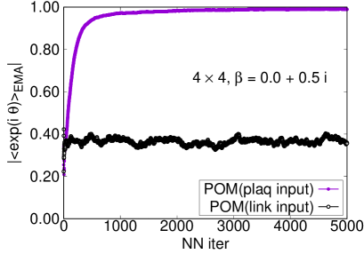
Figure 2 exhibits the neural-network–step-number dependence of the exponential moving average of the average phase factor $\left\langle\exp(i\theta)\right\rangle_{\rm EMA}$ at $\beta=0.0+0.5i$ on a $4\times 4$ lattice as a typical example. The path optimization with the plaquette input successfully enhances $\left\langle\exp(i\theta)\right\rangle_{\rm EMA}$, while that with the link variable input does not. Similar behavior is also observed at other values of $\beta$ on $2\times 2,4\times 4$ and $8\times 8$ lattices. Our result verifies the advantage of the gauge invariant input to the neural network for the 2-dimensional $U(1)$ gauge theory with the complex coupling.

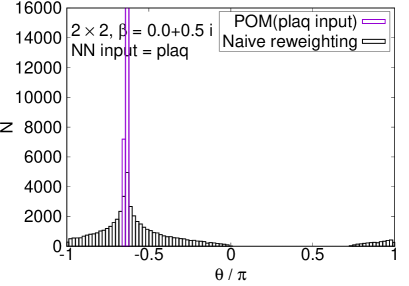
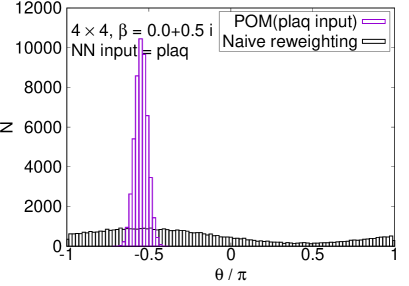
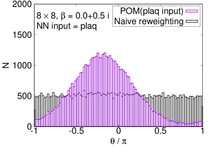
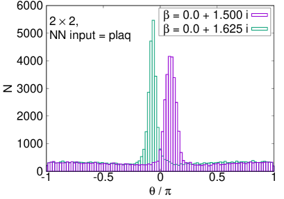
The enhancement with the plaquette input is confirmed in the histogram of the phases, shown in Fig. 3. While the naive reweighting gives a broad distribution of the phase factor, the path optimization significantly sharpens the peak structure. We stress that the POM works even on the $8\times 8$ lattice, where the sign problem is severer. Although the naive reweighting has almost flat dependence on the phase, the POM can still extract a peak structure around $\theta/\pi\sim-0.2$.

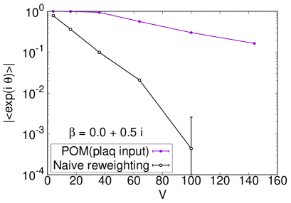
Figure 4 represents the volume dependence of the average phase factor at $\beta=0.0+0.5i$ with additional simulation results on $6\times 6$, $10\times 10$ and $12\times 12$ lattices. The naive reweighting leads to steep exponential fall-off as a function of the volume. The sign problem becomes extremely severer toward the infinite volume limit. The path optimization evidently changes the volume dependence of the average phase factor to be milder. It indicates better control of the sign problem.

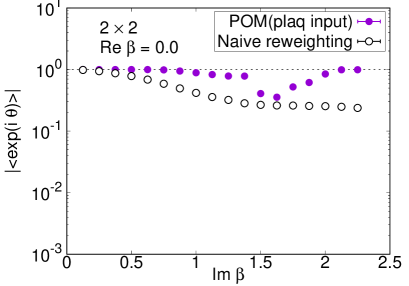
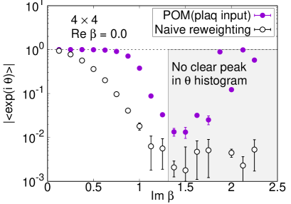
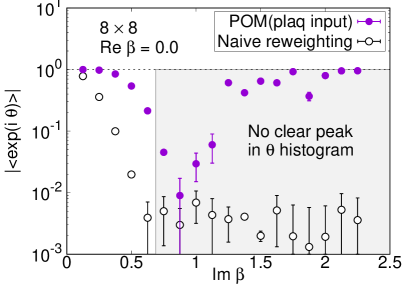
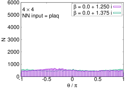
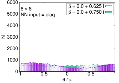
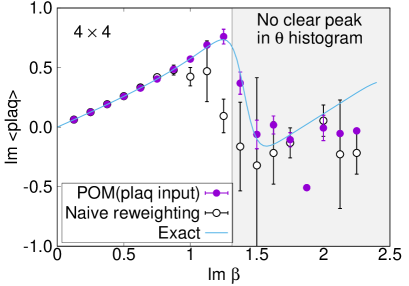
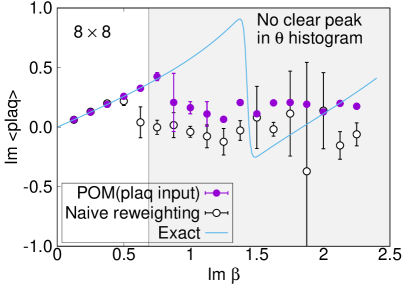
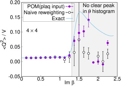
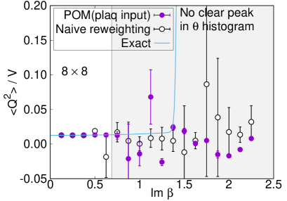
We plot the average phase factors with and without the path optimization as functions of $\mathrm{Im}\,\beta$ in Fig. 5. The average phase factors are enhanced by factors of up to 4 on $2\times 2$, 21 on $4\times 4$, and 27 on $8\times 8$ lattices, respectively. The enhancement decreases, however, as we approach the critical coupling ${\rm Im}\beta_{c}\sim 1.5$ where the partition function becomes zero, corresponding to the Lee-Yang zero. While clear peaks are still visible in the histogram of the phases by the path optimization even at $\beta\sim\beta_{c}$ on $2\times 2$ lattice, no clear peak is obtained and the neural network eventually becomes unstable around $\beta_{c}$ on $4\times 4$ and $8\times 8$ lattices, as displayed in Fig. 6. We need further improvement of the POM around $\beta_{c}$ on large lattices.

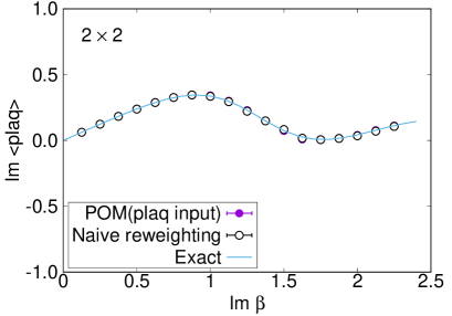
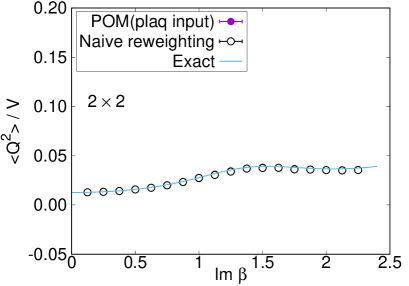
Comparison with the exact solution (4) is accomplished for the expectation values of the plaquette and the topological charge. The result for the plaquette is plotted in Fig. 7 and for the topological charge in Fig. 8. The naive reweighting works in a small $\beta$ region but starts to deviate from the exact value with uncontrolled errors as $\beta$ becomes larger. Our data using the POM agree with the exact solution, as long as we find a peak in the histogram of the phases. The valid region of the POM is definitely extended to larger $\beta$. Deviations from the exact solution are also observed by the path optimization case, if we have no clear peak in the histogram of the phases, where enhancement of the phase factor by the path optimization is still limited to be small or the path optimization is unstable. One reason of the failure is a restriction of the statistics. The machine learning requires more data to find the best path especially for a system with a large degrees of freedom. Another possibility is the effect of the multimodality. Though there can be several regions contributing to the integral (relevant thimbles), the optimized path may emphasize only a part of them. Quantitative evaluation of the systematic errors of the POM result is still difficult and is beyond the scope of this paper. It is an important future work. Nevertheless, these results demonstrate the superiority of the POM over the naive reweighting for the analysis of the $U(1)$ gauge theory with the complex $\beta$.