∎ \sidecaptionvposfiguret
Department of Electrical and Computer Engineering
Center for Translational Cancer Research (TranslaTUM)
Technical University of Munich
81675 Munich, Germany
22email: rune.barnkob@tum.de 33institutetext: Massimiliano Rossi 44institutetext: Department of Physics
Technical University of Denmark
DTU Physics Building 309
DK-2800 Kongens Lyngby, Denmark
44email: rossi@fysik.dtu.dk
General Defocusing Particle Tracking:
Fundamentals and uncertainty assessment
Abstract
General Defocusing Particle Tracking (GDPT) is a single-camera, three-dimensional particle tracking method that determines the particle depth positions from the defocusing patterns of the corresponding particle images. GDPT relies on a reference set of experimental particle images which is used to predict the depth position of measured particle images of similar shape. While several implementations of the method are possible, its accuracy is ultimately limited by some intrinsic properties of the acquired data, such as the signal-to-noise ratio, the particle concentration, as well as the characteristics of the defocusing patterns. GDPT has been applied in different fields by different research groups, however, a deeper description and analysis of the method fundamentals has hitherto not been available. In this work, we first identity the fundamental elements that characterize a GDPT measurement. Afterwards, we present a standardized framework based on synthetic images to assess the performance of GDPT implementations in terms of measurement uncertainty and relative number of measured particles. Finally, we provide guidelines to assess the uncertainty of experimental GDPT measurements, where true values are not accessible and additional image aberrations can lead to bias errors. The data were processed using DefocusTracker, an open-source GDPT software. The datasets were created using the synthetic image generator MicroSIG and have been shared in a freely-accessible repository.
Keywords:
general defocusing particle tracking particle tracking velocimetry defocusing microscopy1 Introduction
Measurement methods based on the imaging of tracer particles in a flow are standard tools in experimental fluid mechanics. Probably the most representative method is the the Particle Image Velocimetry (PIV), introduced in the mid-1980s, which in its basic configuration allows to measure a two-dimensional, two-component (2D2C) flow field by looking at the displacement of tracer particles illuminated by a thin laser sheet adrian1984scattering ; willert1991digital . In the following years, also thanks to the improvement of digital cameras, computers, and image analysis software, a great variety of new techniques derived by PIV has come out, allowing time-resolved, 3D3C measurements, at large or microscopic scale. A good overview can be found in the reference textbook by Raffel et al. raffel2018particle . When the displacements of individual particles are measured, rather than the average particle displacement in interrogation windows, the method is more properly referred to as Particle Tracking Velocimetry (PTV).
Methods derived from PIV or PTV are lately becoming more and more important, not only in experimental fluid mechanics, but also in other disciplines such as medicine, biology, or bio-engineering, in which the experimental characterization of complex fluidic systems, like blood vessels or biochemical microfluidic platforms, is crucial. In this domain, a major role is played by single-camera, 3D PTV methods, which are needed in environments where the flow is three-dimensional and only one optical access, typically through a microscope objective, is available taute2015high ; rossi2017kinematics ; barnkob2018acoustically ; rossi2019interfacial ; liu2019investigation . In the past years, the development of single-camera, 3D particle tracking methods has become a research field on its own cierpka2012particle . The major challenge here is to obtain the depth information from two-dimensional images of particles. Several principles have been proposed to solve this problem, such as holography memmolo2015recent , light-field cameras fahringer2015volumetric ; shi2019volumetric , or image defocusing willert1992three ; pereira2000defocusing ; wu2005three ; zhang2008three ; van2012non ; cierpka2010simple ; rossi2014optimization ; barnkob2015general . Defocusing is a particularly attractive approach, since it does not necessarily require the implementation of special optics or cameras. The main idea is to use optical systems with small depth of field, where the degree of defocusing of the particle images is related to the particles’ depth positions.
A large variety of 3D particle tracking methods relying on defocusing has been proposed. A first notable implementation was the Defocusing Digital PIV, where a three-pinhole mask was used to more efficiently read-out the defocusing information willert1992three ; pereira2000defocusing . Other research groups looked at the changes of the radial intensity profiles of axisymmetric particle images zhang2008three ; van2012non ; afik2015robust . Another method is the Astigmatic PTV, where an astigmatic aberration, introduced by a cylindrical lens, is used to obtain particle image shapes with a characteristic elliptical shape directly related to their depth position cierpka2010simple ; rossi2014optimization .
All these methods share the same principle: The particle image changes shape in a systematic fashion depending on the particle’s depth position. This principle can be generalized to any optics or image type, by constructing a lookup table that maps the particle image shapes with the corresponding depth positions. This approach was introduced by Barnkob et al. barnkob2015general and is referred to as the General Defocusing Particle Tracking (GDPT). The same concept was developed independently by Taute et al. taute2015high to track the 3D motion of bacteria using a standard phase-contrast microscope. Both implementations by Barnkob et al. and Taute et al. used the normalized cross-correlation for comparing the target images with the images in the lookup table; however, different image comparison approaches can be used, and neural networks and artificial intelligence are expected to play a significant role in the future newby2018convolutional ; munoz2019machine .
GDPT has been applied in different fields and by different research groups qiu2019experimental ; volk2018size ; rossi2017kinematics ; barnkob2018acoustically ; boyko2020nonuniform . However, the description of GDPT is limited to the seminal papers in Refs. 3 and 31, and there is a need for a more thorough definition and analysis of the fundamental elements characterizing a GDPT measurement. This step is crucial for a deeper understanding of the method and for future developments and improvements. Moreover, to be able to compare different GDPT algorithms and implementations, standardized assessment schemes and a database of reference images must be established, in analogy to what is already available for PTV or PIV kahler2016main . Consequently, the objective of this work is to fill this gap and provide the basis for further understanding and development of the GDPT method.
In Section 2 we identify the fundamental elements that characterize a GDPT measurement and provide a standardized scheme to assess its uncertainty. Following, in Section 3 we study the uncertainty of the method as a function of image noise and particle image density using synthetic images. Finally, in Section 4 we provide guidelines to assess the uncertainty of GDPT measurements in experimental cases where bias errors are present and the true values are not accessible. The synthetic datasets used in this work are presented in Appendix A and are freely-available to the research community. The datasets are analyzed using DefocusTracker, an open-source GDPT implementation described in Appendix B.
2 Fundamentals of GDPT
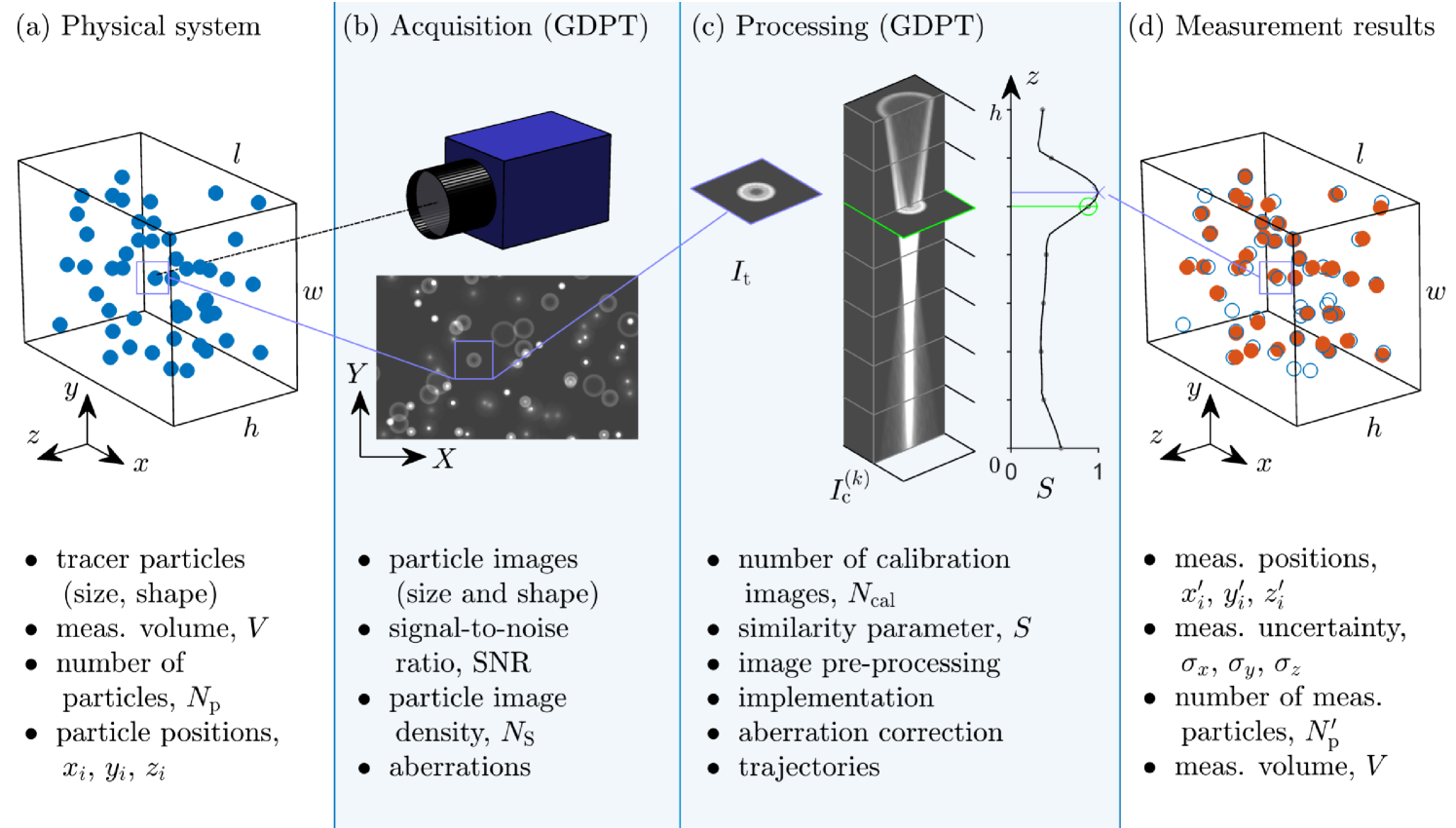
The fundamental principles of a GDPT analysis are outlined in Fig. 1 and involve (a) the physical system under investigation, (b) a single-camera acquisition approach, (c) an image processing approach, and (d) the evaluation of the measurement results. The list of symbols and parameters used in this section is given in Table 1.
2.1 Physical system
The purpose of a 3D particle tracking system is to locate the physical coordinates
| (1) |
of a number of tracer particles inside a measurement volume and to track their displacement in time. The tracking problem will not be discussed here; in GDPT analysis, the particle concentration is relatively low and conventional tracking algorithms can be used. The fundamental analysis in this work concerns only the problem of particle location determination in GDPT. As we consider single-camera acquisition, it is convenient to define the reference frame with two in-plane coordinates, and , perpendicular to the optical axis of the camera objective, and one depth coordinate, , parallel to the optical axis (Fig. 1). The measurement volume can be approximated by a rectangular cuboid with dimensions , being the dimension in the depth direction. The maximum size in the in-plane direction () is set by the field of view of the imaging system. The maximum depth that can be achieved depends on the imaging system, the particle size, and the illumination intensity, and corresponds to the region where the signal of defocused particle images is strong enough to be processed by the image analysis method.
2.2 Acquisition (GDPT)
When using single-camera systems, the tracer particles in the measurement volume are recorded on a single image. For a given optical system, we can define a particle image function which provides the image of one particle depending on its position in the physical space. can be seen as a point spread function defined for one particle, where and are the coordinates in the image space, and where we impose that the center of the particle image is located at for any , , and .
We consider an idealized optical system with no distortions, and where is independent of the in-plane coordinates (Fig. 2(a))
| (2) |
Under this approximation, we can represent a general image , containing a total number of particles, as
| (3) |
where is the magnification of the optical system and where is a term that accounts for background intensity and thermal noise of the camera.
With respect to the final result of a GDPT evaluation, two primary parameters must be considered:
-
•
Signal-to-noise ratio (SNR). Following a convention used in image analysis, we define the SNR as the ratio between the mean particle image signal and the standard deviation of the noise
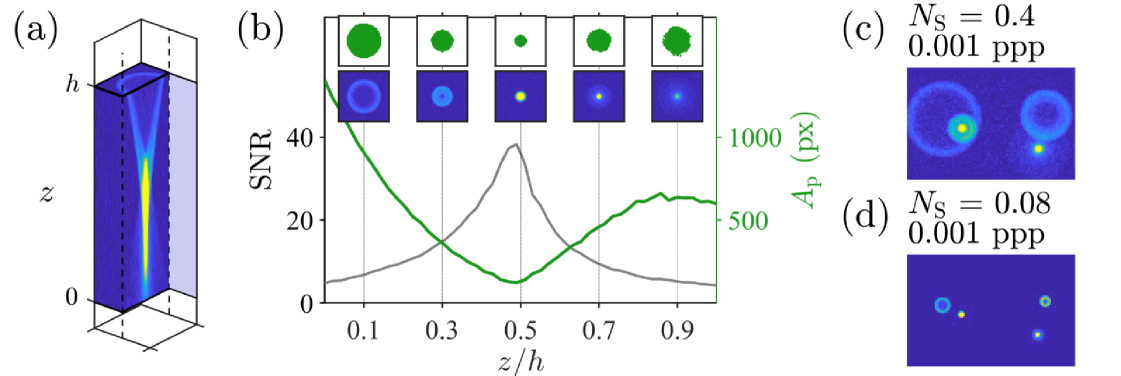
(4) Practically, can be estimated as the standard deviation of the image intensity in a region without particles, and can be calculated as the average intensity of the particle image minus the average background intensity. We can define the boundary of a particle image by setting a threshold, as shown in Fig. 2(b).
-
•
Particle image density . This parameter is often given in particles per pixels (ppp). This approach, however, does not consider the particle image size, which is an important factor in defocusing applications with respect to overlapping particles, as shown in Fig. 2(c-d). For GDPT analysis, it is more convenient to consider the ratio between the sum of the particle image areas and full image area kahler2012uncertainty
(5) Here, is the average of the particle image areas, which can be estimated for instance from the calibration stack. One can easily translate the value in ppp, by dividing it with . It should be noted that this parameter is equivalent to the source density encountered in classical PIV literature adrian1984scattering ; westerweel2000theoretical .
In real optical systems, the approximation in Eq. (2) may not hold as a consequence of optical aberrations. The most common aberrations which are relevant for GDPT applications are:
-
•
Parallax or perspective error. The magnification is not constant across the measurement depth, i.e. objects closer to the lens appear larger on the image. This error is typically small and can be neglected for microscope objective lenses.
-
•
Field curvature. The focal plane is not flat, therefore the measured position must be corrected depending on the particle in-plane position. This effect is relevant in GDPT applications since a field curvature of a few micrometers can have a significant impact in the measurement.
-
•
Distortion. The particle images are distorted as they move away from the image center. This error is difficult to correct in GDPT analysis based on a single calibration stack but is normally not strong in conventional optical setups.
More details about practical strategies to deal with optical aberrations and bias errors are discussed in Section 4.
2.3 Processing (GDPT)
The aim of a GDPT processing is to determine the 3D particle positions from the defocused particle images. The in-plane position can be obtained using one of the many approaches developed for 2D PTV maas1993particle ; ohmi2000particle ; ouellette2006quantitative ; raffel2018particle . The out-of-plane component is determined using a reference set of calibration images and must contain the following elements:
-
1.
A discrete reference set of calibration images, referred to as the calibration stack. This can be seen as a discrete sampling at known positions of the particle image function
(6) is typically obtained experimentally by taking subsequent images of a reference particle which is displaced at known positions, for instance using a motorized focusing stage barnkob2015general .
-
2.
A function or procedure to identify target particle images inside the image . This normally relies on segmentation algorithms that can be applied on raw or filtered/pre-processed images.
-
3.
A function or procedure to quantify the similarity between different images. This is used to rank the calibration images in with respect to their similarity to a given target particle image .
-
4.
A function or procedure to estimate the final depth position of the target particle from the similarity values between and . It should be noted that a simple identification of the most similar image in the stack would produce a discrete output. Interpolation schemes are needed to obtain a continuous output with a “sub-image” resolution, in analogy with what is typically done in digital PIV evaluations to obtain sub-pixel resolution.
More generally, the determination of the depth position in GDPT can be seen as a supervised learning problem, where the calibration stack is the training set used to calibrate a prediction algorithm. The scheme of the prediction algorithm remains the same but it can be trained on different setups just using different calibration stacks. We used in this paper the implementation based on the normalized cross-correlation proposed in Ref. 3, but other approaches using neural networks or more sophisticated classification schemes would be natural improvements of the method.
| Symbol | Description |
|---|---|
| Image area | |
| Particle image area | |
| Normalized cross-correlation maximum | |
| Median filter size | |
| Image | |
| Image background | |
| Particle image function | |
| Calibration image stack | |
| Target particle image | |
| Magnification | |
| Mean particle image signal | |
| Number of calibration images | |
| Number of particles per image | |
| Number of meas. particles per image | |
| Particle image density (source density) | |
| Critical particle image density | |
| Measured particle image density | |
| Meas. uncertainty, in-plane coords. | |
| Local meas. uncertainty, in-plane coords. | |
| Meas. uncertainty, depth coord. | |
| Local meas. uncertainty, depth coord. | |
| Image noise level (standard deviation) | |
| Relative num. of meas. particles | |
| Local relative num. of meas. particles | |
| SNR | Image signal-to-noise ratio |
| / | Similarity parameter / function |
| Measurement volume | |
| , , | Coordinates in physical space |
| , , | Particle coordinates |
| , , | Measured particle coordinates |
| , | Coordinates in image space |
2.4 Measurement results
The result of a GDPT evaluation on a single image, containing a total number of particles, is a set of measured particle coordinates , , , where
| (7) |
where is the measurement error and the same definition applies for the other coordinates. To assess the performance of a GDPT measurement, the following parameters must be considered:
-
1.
The measurement uncertainty in the particle position determination.
-
2.
The relative number of measured particles.
-
3.
The depth of the measurement volume.
For a fair assessment of a GDPT measurement, all these three parameters should be considered, since they are interconnected among each other. For instance, a stricter validation criterion can reduce the error but at the expenses of a smaller number of measured particles.
-
•
Measurement uncertainty. When the true particle position is known, as in the case of synthetic images, the measurement uncertainty in the determination of one coordinate is normally given in terms of the root-mean-square of the error
(8) where indicates summation over the measured values and is equal to the total number of measured particles . Since the particle images have different shapes, a non-uniform uncertainty along is expected and it is useful to define a local uncertainty
(9) with
(10) Eq. (9) indicates the uncertainty associated to a bin centered at and having a width of . The same applies for the uncertainty of the in-plane coordinates and . For particle images with rotational symmetry, we can assume . Note that Eqs. (8) and (9) give the total error, since the true values are used. If the uncertainty is calculated around a mean value, as in case of experimental images, the uncertainty does not take into account bias errors. A discussion about how to apply these formulas to experimental images is presented in Section 4.
-
•
Relative number of measured particles. This is defined as the ratio between the number of measured particles and the total number of particles in one image
(11) Also in this case it is useful to define a local defined as
(12) The relative number of measured particles tends to decrease as the particle concentration is increased, due to the more frequent occurrence of overlapping particle images. For a given GDPT implementation, there will be a critical particle image density above which the number of measured particles starts to decrease. This sets the maximum possible seeding density that should be used for that implementation. Furthermore, it should be noted that is not directly accessible in experimental images, where only the number of measured particles is available.
-
•
Measurement volume. The choice of the depth of the measurement volume affects the total number of particles to be measured and, consequently, the number of overlapping particles and the measurement uncertainty. For instance, a large depth can include highly-defocused particle images, which have a smaller SNR and are more difficult to detect. To fairly estimate the uncertainty of a given implementation, the measurement depth on which it is applied must be indicated. In GDPT systems, is practically set by the lowest and highest coordinate in the stack.
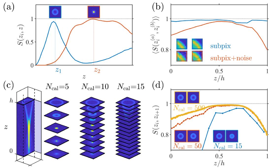
2.5 Concept of similarity
The calibration stack represents a discrete sampling of the particle image function across . The depth position of a particle is obtained by comparing a target particle image with the images in the stack using a similarity function , usually normalized between 0 and 1, with 1 being the perfect match (Fig. 3(a)). In an ideal case, the measurement resolution can be increased indefinitely by increasing the number of images in the stack (Fig. 3(c)). In a real case, however, beyond a certain the difference in shape between two neighbor images will be smaller than the difference induced by the image noise and in-plane image discretization (i.e. the light-intensity distribution is discretized into pixels).
This concept is illustrated in Fig. 3(b), where the self-similarity, i.e. the average between particle images at the same height but different in-plane positions, is shown as a function of . Even in the case with no noise (blue line), is not unity due to tiny differences induced by sub-pixel displacements of the particle images. By adding noise (red line, ), decreases significantly, especially in regions where the SNR is lower. A way to check whether a calibration stack is over-sampling , is to calculate the similarity between neighbor images in the stack, i.e., . In the example in Fig. 3(d), the stack with (orange line) is clearly over-sampled, since it coincides with the self-similarity curve in Fig. 3(b). Further refining the stack will not bring any advantage. For (blue line), the between neighbor images is small, showing that the stack under-samples the particle image function. The stack with (red line) is a better compromise, with a slightly under-sampled region for and over-sampled above.
3 Standardized uncertainty assessment using synthetic images
For a complete assessment of the effect of , SNR, and on the final results, it is necessary to look at the final error in the determination, which is also affected by the choice of the similarity function and the practical implementation of the method (e.g. algorithms used, interpolation schemes, and smoothing). In this section, we present a systematic procedure based on synthetic images to address these aspects. Guidelines for the uncertainty assessment in experimental cases is provided in the next section.
The particle images are generated using MicroSIG rossi2019synthetic . We consider here three datasets to analyze, respectively, the effect of noise, particle concentration, and background intensity gradients. The datasets are freely available111The datasets can be downloaded through https://defocustracking.com/., more details are given in Appendix A. The datasets are analyzed using DefocusTracker which is an open-source GDPT implementation. As similarity parameter, DefocusTracker uses , the maximum of the normalized cross-correlation between two images; for more details, see Appendix B.
3.1 Calibration sampling and signal-to-noise ratio
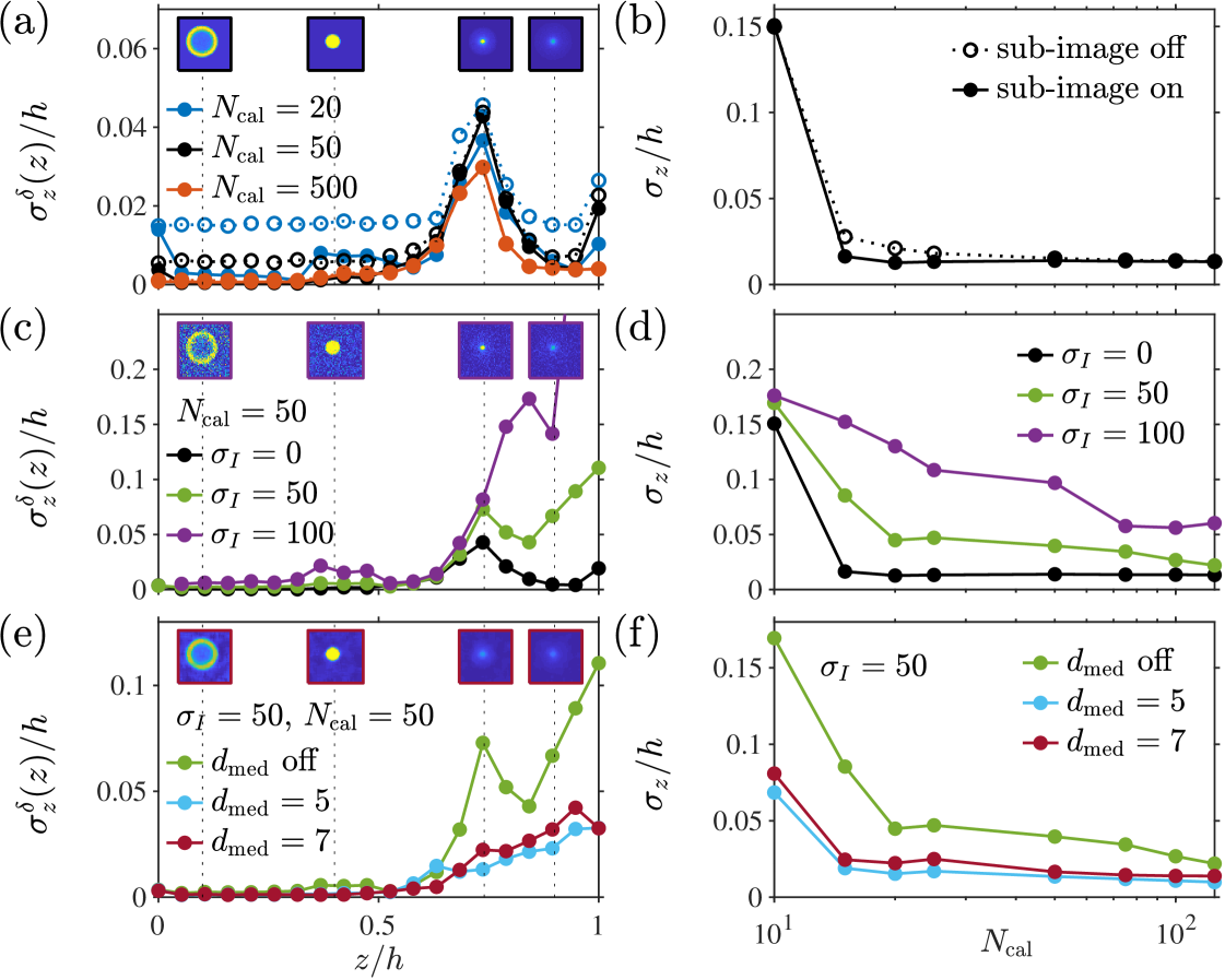
In this section we evaluate the effect, on the depth coordinate determination, of the number of calibration images and sub-image interpolation along with the influence of image noise. More specifically, we analyze Dataset I (Fig. 8(a) in Appendix A) where particle images do not overlap; thus all the particles are detected, i.e., .
To isolate the different effects, we first analyze images with no noise, i.e. . The results are shown in Fig. 4(a), where we plot the local depth coordinate uncertainty as a function of along with a selection of the corresponding particle image shapes. The results are shown when using , 50, or 500 calibration images with (points) and without (open circles) the use of sub-image interpolation. It may be noted that the defocused particle images have a sharp ring shape below the focal position (low ) and blurred Gaussian-like shape above (high ). This is due to the spherical aberration which is present in many optical systems and included in MicroSIG rossi2019synthetic . Detecting the shape differences for blurred particle is more difficult, which explains the larger uncertainty in regions with .
Generally, increasing leads to a decreasing local uncertainty , but e.g. for , the use of a sub-image detection scheme can lead to better results for lower which is seen by a better performance for (blue lines) than for (black lines) or (red lines). The use of a sub-image interpolation scheme allows for a continuous determination and does in general yield lower uncertainties up to a certain value of . This is shown in Fig. 4(b), where we show the depth coordinate uncertainty as a function of . As approaches 200, the uncertainty, with and without the use of a sub-image scheme, converges to the same value.
We now fix the number of images in the calibration stack to and analyze images with increasing noise levels. The results are presented in Fig. 4(c). Not surprisingly, the local depth coordinate uncertainty increases with a decreasing SNR. As explained before, the local uncertainty for larger values of is larger due to the blurred Gaussian-like shape of the particle images. The effect of noise on the local uncertainty naturally propagates into the total uncertainty as seen in Fig. 4(d). Clearly, as the noise level increases, a larger is needed in order to reach a converging uncertainty .
Lastly, to explore the reduction of noise through image pre-processing, we now fix the noise level to and apply different median filters to the images. We illustrate this in Fig. 4(e) where we apply a median filter of (with equal to 5 or 7) to both the calibration and the measurement images. The median filter decreases the impact of noise in the local uncertainty , in some region even as much as one order of magnitude. Evidently, the filter size has an optimum between averaging out noise and actual particle image features — this is seen by the presence of some slightly lower values of for than for . This is confirmed in Fig. 4(f), where the same trend is seen for the average uncertainty .
3.2 Particle image overlap and particle concentration
After investigating the effect of noise and , we now analyze the more experimentally-realistic case where the presence of overlapping particle images is possible. In particular we use the noise-less () Dataset II (Fig. 8(b)) to assess the GDPT uncertainties as a function of increasing particle concentration while keeping the number of calibration images fixed (). We consider here particle image densities up to , corresponding to 0.001 particles per pixels. As the particle concentration increases, the number of overlapping particle images increases concurrently. This leads to lower similarities between target particle images and calibration images, which furthermore leads to larger errors in the determination of the -coordinates. By setting a higher threshold on the accepted values of , poorly-determined -coordinates can be removed to increase the determination accuracy but with the cost of lowering the number of measured particles .
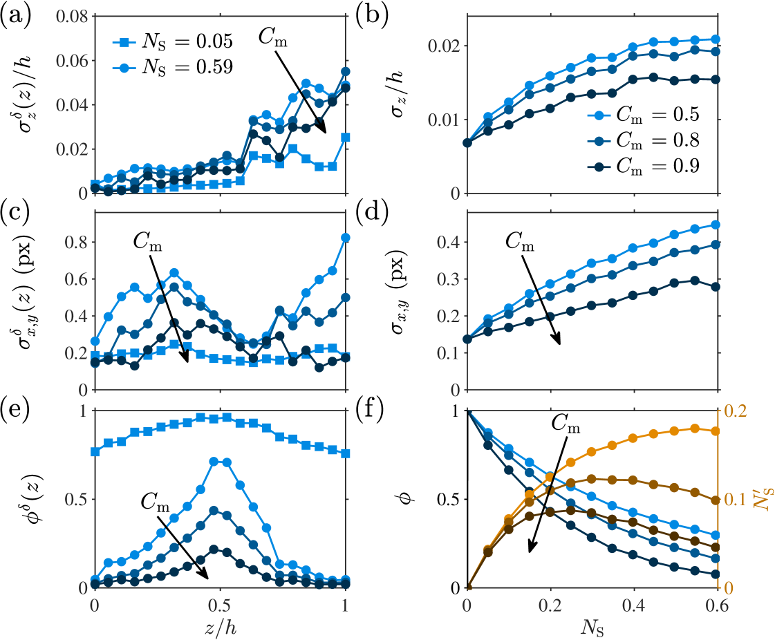
In Figs. 5(a), 5(c), and 5(e), we show the local uncertainties and , and the local relative number of measured particles for two particle image densities of (squares) and (circles), respectively. As is increased from 0.05 to 0.59, the local errors and are consistently increasing, while the local relative number of measured particles is consistently decreasing. As the threshold on is increased, both , , and are decreasing as expected. The same trend is confirmed in Figs. 5(b), 5(d), and 5(f), where the uncertainties and , and the relative number of measured particles are computed as a function of the particle image density and , 0.8, and 0.9, respectively. In addition, we see in Fig. 5(f) that as increases, the measured particle image density (orange colors) reaches a peak, e.g., for when . In fact, as the particle concentration is increased, the number of particles in the image increases but so does the number of outliers or not-detectable particle images due to the increased number of overlapping particle images that cannot be processed. This can be seen as a critical value, denoted here as , that sets the maximum particle image density that can be used with those settings.
3.3 Variations in image intensity
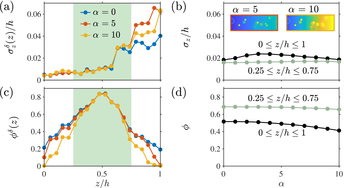
Experimental measurement images are prone to variations in image light intensity, for example, if the image illumination is inhomogeneous over the image plane or if the illumination amplitude changes over time. This can eventually affect the accuracy of defocusing-based particle detection, but depends on the type of image intensity variation and applied detection algorithm. In this section, we assess the GDPT measurement uncertainties when analyzing measurement images with an applied linear light intensity gradient of increasing steepness. More specifically, we use Dataset III (Fig. 8(c)), which is based on the images in Dataset II for and to which an intensity gradient has been applied.
Figures 6(a) and 6(c) show the local depth coordinate uncertainty and the local relative number of measured particles . For small , the changes are small as expected from the fact that the normalized cross-correlation is insensitive to changes in intensity level. However, as increases, the intensity gradient becomes comparable to the intensities of the particle image features. This affects the uncertainty and the number of measured particles specially in regions where the SNR is low (outside the green area in Fig. 6(a) and (c)). Overall, the effect of intensity gradient is small in the region with large SNR, as shown in Fig. 6(b) and (d). Note also the previously discussed connection between the uncertainty and number of measured particles, e.g., without considering the latter, one would erroneously observe in Fig. 6(b) a better performance for than for .
4 Uncertainty assessment on experimental images
The fundamental uncertainty assessment presented in this work is only perfectly-applicable to synthetic images. When moving to experimental images, the true values are obviously unknown and additional factors can bias the measurement result. In this section, we briefly discuss the most relevant sources of bias error that should be taken into account and provide guidelines about how to estimate the uncertainty on experimental images.
4.1 Refractive index
A common way to obtain the calibration stack experimentally is to use one particle at a fixed position (e.g. stuck to a wall) and to move the objective lens at different depth positions. The reference coordinates are obtained from the reading of the scanning device. During the measurement, however, the situation is reversed: The objective lens is fixed and the particles move. This has consequences if the immersion medium of the lens is different from the medium where the particles are dispersed, and a correction coefficient must be multiplied to the measured . In most applications, this coefficient is equal to the ratio between the refractive index coefficient of the fluid (typically water) and the one of the immersion medium of the lens (typically air) rossi2012effect .
4.2 Aberrations
In real applications, the particle image function is not the same across in-plane positions due to optical aberrations. The more straightforward way to address this problem would be to take multiple calibration stacks for different in-plane positions; however, this approach is difficult to implement. First, the size of the calibration stack would increase considerably and so the time necessary for the calibration (a particle must be scanned in different positions). Second, higher complexity and computational costs would be needed to navigate the different calibration stacks and an interpolation scheme must be implemented to cover the entire area of the sensor (only a discrete set of in-plane positions can be taken). Future implementations of the GDPT method using neural network might be able to tackle this task.
In many practically applications, however, the aberrations are weak and a single calibration stack (typically obtained in the center of the image) can be used in the whole image area rossi2019interfacial ; barnkob2018acoustically ; qiu2019experimental . Additional bias errors due to field curvature or perspective errors can be corrected using a reference experiment, for instance, using a fixed array of tracer particles on a flat plane perpendicular to the optical axis and scan it at different depth positions.
In microfluidics applications, where microscope objectives are used, the perspective error is typically negligible, but the field curvature can give errors of few microns cierpka2010calibration , which might be relevant at those scales. If the measurements are performed on a straight microchannel, one practical way to correct this bias is by a direct measurement of a Poiseuille flow inside the duct. In this case, we know that the streamlines in such flow must be straight lines, and we can use this information to determine and correct the field curvature.
4.3 Uncertainty estimation
To estimate the measurement uncertainty of an experimental GDPT setup, we can use Eqs. (8) and (9), but we need to estimate the unknown true values. A practical approach can be to measure particle displacements in flows having zero velocity in one direction. We can estimate then the displacement uncertainty, considering 0 as the true value. Modeling the error as normally distributed, the positioning uncertainty will be equal to the displacement error divided by . Of course, particular care should be taken with reducing as much as possible the bias errors and eliminating false positive with an appropriate outlier rejection scheme. Together with the uncertainty, it is important to indicate the depth of the measurement volume. When it is possible to estimate , for instance, if the experimental particle concentration is known, the relative number of measured particles can be calculated; otherwise, should be indicated.
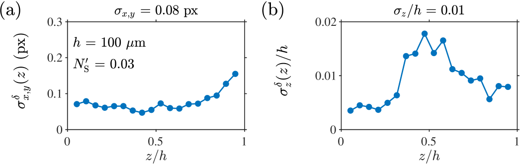
We give an example of the uncertainty estimation on experimental measurements in Fig. 7 using data from Ref. 3. The data contain GDPT measurements of a Poiseuille flow in a microchannel with a rectangular cross-section of 380 m 100 m. The flow is directed along the direction and the uncertainty was estimated along the perpendicular directions and , i.e., the directions of zero flow velocity. For a (very few overlapping particles) and across a height of m, we obtained uncertainties px and , in good agreement with the values obtained in the analysis of the synthetic images.
5 Conclusions
We have identified the fundamental elements characterizing a GDPT measurement; these are the number of images in the calibration stack , the image signal-to-noise ratio SNR, the particle image density , and the function chosen to evaluate the similarities between calibration and target images. For the evaluation of GDPT measurements, we presented an assessment scheme encompassing the measured coordinate uncertainties, the relative number of measured particles, and the depth of the measurement volume.
For a practical implementation of the presented assessment scheme, we created a group of freely-available synthetic image datasets and we used them to study the performance of the GDPT software DefocusTracker. The fundamental findings of the study are: (i) There is an optimal number of images in the calibration stack, including more images will not reduce the measurement uncertainties, (ii) the presence of overlapping particle images increases significantly the uncertainty; using a stricter criterion to accept valid measured particles can help to improve the accuracy but at the expense of the number of measured particles, and (iii) for each setting, one can extrapolate a critical particle image density beyond which the number of measured particle decreases. The most relevant quantitative results of the study are summarized in Table LABEL:tab:performance_defocustracker.
| (px) | ||||||
|---|---|---|---|---|---|---|
| 0.5 | 50 | 50 | - | 0.152 | 0.014 | 1 |
| 0.5 | 50 | - | 0.545 | 0.436 | 0.021 | 0.330 |
| 0.9 | 50 | - | 0.248 | 0.213 | 0.013 | 0.353 |
We provided guidelines to assess the uncertainty of GDPT measurements in experimental cases where bias errors can be present and in contrary to synthetic images, the true values are not accessible. Bias errors occur because of discrepancies between calibration and target images induced by optical aberrations. This should be taken into account, e.g. by implementing multiple calibration stacks for strong aberrations, or by implementing reference experiments for weak aberrations where one single calibration stack can still be used. To estimate experimental uncertainties, one needs to estimate the true values. This is possible for instance by looking at a velocity flow fields with null velocity in one measurement direction.
In conclusion, this work provides the tools for a more aware use of GDPT and is an important step toward the further development of the method in terms of accuracy, efficiency, and processing speed. Next steps include the expansion of the datasets to temporal-coherent data, non-monodisperse particles, and experimental data, for instance including biological cells for use of GDPT in biomedical sciences.
Acknowledgements.
This work was supported by the European Union’s Horizon 2020 Research and Innovation Programme under the Marie Sklodowska-Curie Grant No. 713683 (COFUNDfellowsDTU).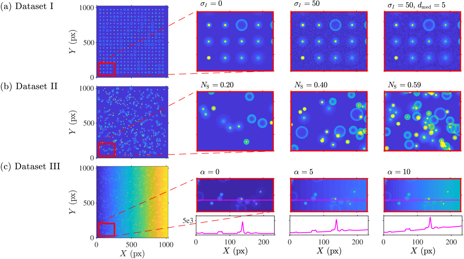
Appendix A Datasets for standardized evaluation of GDPT methods
In this section, we introduce a group of three datasets and corresponding calibration images for evaluating the performance of a GDPT implementation as a function of different signal-to-noise ratio SNR, particle image density , and background intensity gradients. The datasets do not include the effect of field curvature or image aberrations. The datasets are meant to act as a reference set for the scientific community and are freely available222The datasets can be downloaded through https://defocustracking.com/..
The datasets are based on synthetic images created using MicroSIG, which is a Synthetic Image Generator (SIG) using ray tracing and a simplified spherical lens model to obtain realistic defocused or astigmatic particle images rossi2019synthetic . MicroSIG is open source and can be downloaded at gitlab.com/defocustracking. In this work, we consider bright, monodisperse particles of diameter , which is the most common case in velocimetry applications. All datasets share the same basic MicroSIG settings in terms of particle diameter ( = 2 m), objective lens (magnification = 10, numerical aperture NA = 0.3, focal length = 350 m), and sensor settings (pixel size of 6.5 m, = 500 counts). The settings have been chosen since they simulate experimental conditions that are representative for a large number of applications in microfluidics. The simulated measurement depth m is kept the same for all datasets.
The three datasets are shown in Fig. 8. In order to ensure the same level of statistical significance, all datasets contain 20,000 particles for each set of parameters. The three datasets are:
-
•
Dataset I. This dataset contains measurement images for 3 different noise levels . Each measurement image contains 361 particle images located at random , , and positions. The and coordinates are loosely constraint on a grid to exclude particle image overlapping. The dataset is suitable for analyzing the depth coordinate precision and how it depends on the image noise level , number of calibration images , and method parameters such as image filtering and sub-image approach for the depth coordinate determination.
-
•
Dataset II. This dataset contains 12 subsets of measurement images of particles with randomly distributed , , and coordinates, thus including particle image overlapping. Each subset corresponds to a specific particle image density and contains a certain number of measurement images in order to have an overall number of 20,000 particles. We start with a subset of 1200 images at and end with a subset of 100 images at . This dataset is suitable for analyzing the relative number of measured particles and depth coordinate uncertainty as a function of increasing particle image density.
-
•
Dataset III. This dataset contains 10 subsets of 34 measurement images of 600 particles () with randomly distributed , , and coordinates. Each subset has a superimposed linear light-intensity gradient along the horizontal direction defined as
(13) where is a parameter accounting for the gradient intensity. The impact of can be better appreciated by normalizing its value with the mean particle image intensity divided by the characteristic size of the particle images
(14) A value of indicates a light-intensity gradient on the same order of magnitude of the intensity gradient in the particle images. For this dataset we have ranging from 1 to 10, corresponding to ranging from 0.16 to 1.6.
-
•
Calibration images. The set of calibration images provides the calibration images for analyzing the Datasets I–III with GDPT. It contains calibration image stacks for 3 different noise levels and 12 different numbers of calibration images .
Appendix B DefocusTracker
The GDPT implementation used in this work is the Version 1.0 of DefocusTracker, which is a MATLAB implementation published under the open-source license and available at defocustracking.com. The implementation is based on the normalized cross-correlation for image comparison and a polynomial scheme for sub-image interpolation. In order to work fast and robustly, the implementation uses a cross-correlation prediction scheme based on the set of calibration images; for more details, see Ref. 25. DefocusTracker allows multiple processing iterations using different similarity parameter thresholds to improve the detection of overlapping particles; however, in this work we limit ourselves to one iteration and a single similarity parameter threshold. The implementation allows image noise filter through Gaussian and median filter, though in this work we utilize only the latter. In addition, DefocusTracker allows the determination of particle trajectories through a nearest-neighbor tracking scheme. We do not perform tracking of particles across the image frames in this work, but it is important to mention that using predictive tracking approaches can increase the performance of particle detection as well.
In DefocusTracker the similarity parameter between two images and , is defined as the peak maximum of their normalized cross-correlation function . Here and are the in-plane coordinates in correlation space. Following the seminal paper by Lewis in 1995 Lewis1995fast , the normalized cross-correlation takes the form
| (15) |
where and are the mean image intensities of and , respectively. The correlation function has its peak maximum at the position of best match between the images and the amplitude of the peak maximum ranges from 0 to 1, where 1 indicates a perfect match. A key advantage of the normalized cross-correlation function is that it is robust against light-intensity fluctuations such as inhomogeneous light distribution.
References
- (1) Adrian, R.J.: Scattering particle characteristics and their effect on pulsed laser measurements of fluid flow: speckle velocimetry vs particle image velocimetry. Applied optics 23(11), 1690–1691 (1984)
- (2) Afik, E.: Robust and highly performant ring detection algorithm for 3d particle tracking using 3D microscope imaging. Scientific reports 5(1), 1–9 (2015)
- (3) Barnkob, R., Kähler, C.J., Rossi, M.: General defocusing particle tracking. Lab on a Chip 15(17), 3556–3560 (2015)
- (4) Barnkob, R., Nama, N., Ren, L., Huang, T.J., Costanzo, F., Kähler, C.J.: Acoustically driven fluid and particle motion in confined and leaky systems. Physical Review Applied 9(1), 014027 (2018)
- (5) Boyko, E., Eshel, R., Gat, A.D., Bercovici, M.: Nonuniform electro-osmotic flow drives fluid-structure instability. Physical Review Letters 124(2), 024501 (2020)
- (6) Cierpka, C., Kähler, C.: Particle imaging techniques for volumetric three-component (3D3C) velocity measurements in microfluidics. Journal of visualization 15(1), 1–31 (2012)
- (7) Cierpka, C., Rossi, M., Segura, R., Kähler, C.: On the calibration of astigmatism particle tracking velocimetry for microflows. Measurement Science and Technology 22(1), 015401 (2011)
- (8) Cierpka, C., Segura, R., Hain, R., Kähler, C.J.: A simple single camera 3C3D velocity measurement technique without errors due to depth of correlation and spatial averaging for microfluidics. Measurement Science and Technology 21(4), 045401 (2010)
- (9) Fahringer, T.W., Lynch, K.P., Thurow, B.S.: Volumetric particle image velocimetry with a single plenoptic camera. Measurement Science and Technology 26(11), 115201 (2015)
- (10) Kähler, C.J., Astarita, T., Vlachos, P.P., Sakakibara, J., Hain, R., Discetti, S., La Foy, R., Cierpka, C.: Main results of the 4th international piv challenge. Experiments in Fluids 57(6), 97 (2016)
- (11) Kähler, C.J., Scharnowski, S., Cierpka, C.: On the uncertainty of digital PIV and PTV near walls. Experiments in fluids 52(6), 1641–1656 (2012)
- (12) Lewis, J.P.: Fast normalized cross-correlation. Proceedings of Vision interface 10(1), 120–123 (1995)
- (13) Liu, J., Reisbeck, M., Hayden, O.: Investigation of mechanical and magnetophoretic focusing for magnetic flow cytometry. Current Directions in Biomedical Engineering 5(1), 353–355 (2019)
- (14) van Loenhout, M.T., Kerssemakers, J.W., De Vlaminck, I., Dekker, C.: Non-bias-limited tracking of spherical particles, enabling nanometer resolution at low magnification. Biophysical journal 102(10), 2362–2371 (2012)
- (15) Maas, H., Gruen, A., Papantoniou, D.: Particle tracking velocimetry in three-dimensional flows. Experiments in fluids 15(2), 133–146 (1993)
- (16) Memmolo, P., Miccio, L., Paturzo, M., Di Caprio, G., Coppola, G., Netti, P.A., Ferraro, P.: Recent advances in holographic 3D particle tracking. Advances in Optics and Photonics 7(4), 713–755 (2015)
- (17) Muñoz-Gil, G., Garcia-March, M.A., Manzo, C., Martín-Guerrero, J.D., Lewenstein, M.: Machine learning method for single trajectory characterization. New Journal of Physics 22(1), 013010 (2020)
- (18) Newby, J.M., Schaefer, A.M., Lee, P.T., Forest, M.G., Lai, S.K.: Convolutional neural networks automate detection for tracking of submicron-scale particles in 2D and 3D. Proceedings of the National Academy of Sciences 115(36), 9026–9031 (2018)
- (19) Ohmi, K., Li, H.Y.: Particle-tracking velocimetry with new algorithms. Measurement Science and Technology 11(6), 603 (2000)
- (20) Ouellette, N.T., Xu, H., Bodenschatz, E.: A quantitative study of three-dimensional lagrangian particle tracking algorithms. Experiments in Fluids 40(2), 301–313 (2006)
- (21) Pereira, F., Gharib, M., Dabiri, D., Modarress, D.: Defocusing digital particle image velocimetry: a 3-component 3-dimensional DPIV measurement technique. application to bubbly flows. Experiments in Fluids 29(1), S078–S084 (2000)
- (22) Qiu, W., Karlsen, J.T., Bruus, H., Augustsson, P.: Experimental characterization of acoustic streaming in gradients of density and compressibility. Physical Review Applied 11(2), 024018 (2019)
- (23) Raffel, M., Willert, C.E., Scarano, F., Kähler, C.J., Wereley, S.T., Kompenhans, J.: Particle image velocimetry: a practical guide. Springer (2018)
- (24) Rossi, M.: Synthetic image generator for defocusing and astigmatic PIV/PTV. Measurement Science and Technology 31(1), 017003 (2019)
- (25) Rossi, M., Barnkob, R.: Toward automated 3D PTV for microfluidics. 13th International Symposium on Particle Image Velocimetry — ISPIV 2019, Munich, Germany, July 22-24, 2019, pp. 1456–1462
- (26) Rossi, M., Cicconofri, G., Beran, A., Noselli, G., DeSimone, A.: Kinematics of flagellar swimming in euglena gracilis: Helical trajectories and flagellar shapes. Proceedings of the National Academy of Sciences 114(50), 13085–13090 (2017)
- (27) Rossi, M., Kähler, C.J.: Optimization of astigmatic particle tracking velocimeters. Experiments in fluids 55(9), 1809 (2014)
- (28) Rossi, M., Marin, A., Kähler, C.J.: Interfacial flows in sessile evaporating droplets of mineral water. Physical Review E 100(3), 033103 (2019)
- (29) Rossi, M., Segura, R., Cierpka, C., Kähler, C.J.: On the effect of particle image intensity and image preprocessing on the depth of correlation in micro-PIV. Experiments in fluids 52(4), 1063–1075 (2012)
- (30) Shi, S., Ding, J., New, T., Liu, Y., Zhang, H.: Volumetric calibration enhancements for single-camera light-field PIV. Experiments in Fluids 60(1), 21 (2019)
- (31) Taute, K., Gude, S., Tans, S., Shimizu, T.: High-throughput 3D tracking of bacteria on a standard phase contrast microscope. Nature communications 6, 8776 (2015)
- (32) Volk, A., Kähler, C.J.: Size control of sessile microbubbles for reproducibly driven acoustic streaming. Physical Review Applied 9(5), 054015 (2018)
- (33) Westerweel, J.: Theoretical analysis of the measurement precision in particle image velocimetry. Experiments in Fluids 29(1), S003–S012 (2000)
- (34) Willert, C., Gharib, M.: Three-dimensional particle imaging with a single camera. Experiments in Fluids 12(6), 353–358 (1992)
- (35) Willert, C.E., Gharib, M.: Digital particle image velocimetry. Experiments in fluids 10(4), 181–193 (1991)
- (36) Wu, M., Roberts, J.W., Buckley, M.: Three-dimensional fluorescent particle tracking at micron-scale using a single camera. Experiments in Fluids 38(4), 461–465 (2005)
- (37) Zhang, Z., Menq, C.H.: Three-dimensional particle tracking with subnanometer resolution using off-focus images. Applied optics 47(13), 2361–2370 (2008)