[2]\fnmXinmin\surYang
1]\orgdivCollege of Mathematics, \orgnameSichuan University, \orgaddress\cityChengdu, \postcode610065, \countryChina
[2]\orgdivSchool of Mathematical Sciences, \orgnameChongqing Normal University, \orgaddress\cityChongqing, \postcode401331, \countryChina
General inertial smoothing proximal gradient algorithm for the relaxation of matrix rank minimization problem
Abstract
We consider the exact continuous relaxation model of matrix rank minimization problem proposed by Yu and Zhang (Comput.Optim.Appl. 1-20, 2022). Motivated by the inertial techinique, we propose a general inertial smoothing proximal gradient algorithm(GIMSPG) for this kind of problems. It is shown that the singular values of any accumulation point have a common support set and the nonzero singular values have a unified lower bound. Besides, the zero singular values of the accumulation point can be achieved within finite iterations. Moreover, we prove that any accumulation point of the sequence generated by the GIMSPG algorithm is a lifted stationary point of the continuous relaxation model under the flexible parameter constraint. Finally, we carry out numerical experiments on random data and image data respectively to illustrate the efficiency of the GIMSPG algorithm.
keywords:
Smoothing approximation, Proximal gradient method, Inertial, Rank minimization problem1 Introduction
In the recent years, much work has been dedicated to the matrix rank minimization problem which emerge in many applications, especially in computer vision Zheng_Y and matrix completion Recht . Lots of models, methods and its variants have been studied, one can refer to the literaturesMa_S ; Cai_J ; Mesbahi ; Lai_M ; Fornasier_M ; Ma_T ; Ji_S ; Lu_Z ; He_Y ; Zhao_Q , in detail, the matrix rank minimization problem can be represented as
| (1) |
where denotes the number of nonzero singular values.
In this paper, we concentrate on the exact continuous relaxation of matrix rank minimization problem proposed in Yu_Q_Zhang_X , that is the following nonconvex relaxation problem,
| (2) |
where and is convex and not necessairly smooth, is a positive parameter. is an exact continuous relaxation of the matrix rank minimization problem. The capped- function with given is
| (3) |
It is observed that in (3) can be seen as a DC function, that is
| (4) |
with and . When the matrix is to be diagonal, the problem (2) is reduced to the exact continuous relaxation model of regularization problem which was given in Bian_W_Chen_X , i.e.,
| (5) |
where and is defined as for . In Bian_W_Chen_X , one proposed the efficient smoothing proximal gradient method to solve this kind of problem with box constraint.
In Zhang_J , the authors established the smoothing proximal gradient method with extrapolation (SPGE) algorithm for solving (5). The extrapolation coefficient can be obtained . Further, under more strict condition of the extrapolation coefficient which includes the extrapolation coefficient in sFISTA with the fixed restart ODonoghue , it is proved that any accumulation point of the sequence generated by SPGE is a lifted stationary point of (5). Besides, the convergence rate based on the proximal residual is developed. Since the penalty item of problem (2) is nonconvex for a fixed in (12), the framework of SPGE algorithm in Zhang_J can not be directly applied to the matrix case.
As we know, incorporating inertial item which is also called extrapolation item to the proximal gradient method is a popular technique to improve the efficiency of proximal gradient algorithm for solving the following composition optimization problem,
| (6) |
where is a smooth with Lipschitz continuous gradient and possibly nonconvex function, is a proper closed, and convex function. The composition structure that one item is smooth convex and the other is convex makes the proximal gradient method Parikh_N_Boyd_S widely used. Specifically, the updating scheme can be read as:
where is the stepsize. Throughout this paper, the proximal mapping Parikh_N_Boyd_S of is defined as
where and . The accelerated proximal gradient method for convex optimization problems have been well studied Nesterov_Y0 ; Nesterov_Y1 . In particular, Beck and Teboulle Beck_A_Teboulle_M established the remarkable Fast Iterative Shrinkage-Thresholding Algorithm (FISTA) for the convex case which was based on the Nesterov’s method Nesterov_Y1 ; Nesterov_Y . Some variants of FISTA have been developed by choosing appropriate extrapolation parameters, we refer the readers to Chambolle_A_Dossal_C ; Liang_J_and_C_B and their references therein. In Wu_Z_Li_M , under the proper parameter constraints, Wu and Li established the proximal gradient algorithm with different extrapolation (PGe) coeifficients on the proximal step and gradient step for solving the problem (6) when the smooth component is nonconvex and the nomsooth component is convex. The general framework is given as follows:
| (7) |
where are the extrapolation coefficients, and is the stepsize. In Wu_zhongming , the authors further developed the inertial Bregman proximal gradient method for minimizing the sum of two possible nonconvex functions. In their method, the generalized Bregman distance replaces the Euclidean distance and two different inertial items on the proximal step and gradient step are taken respectively.
For matrix case, Toh and Yun Toh_K_C_Yun_S proposed the accelerated proximal gradient algorithm for the following convex problem:
| (8) |
where is a convex and smooth function with Lipschitz continuous gradient and is a proper closed convex function. The problem arises in applications such as in matrix completion problems Toh_K_C_Yun_S , multi-task learning A_Argyriou and principal component analysis (PCA) Mesbahi ; Xu_H . When the matrix is diagonal, the problem is reduced to the vector optimization problem (6).
Since optimization problem (2) is a matrix generalization of the vector optimization problem (5), it is natural for us to explore the possibility of extending some of the algorithms developed for problem (5) to solve problem (2). We observe that the loss function in above require a restrictive assumption that the function is smooth, it is difficult to apply the proximal gradient method directly for problem (2). Fortunately, the smoothing approxitation methods proposed in Chen_X can overcome the dilemma. Smoothing approximation method is an efficient method which is widely used in other problems. One can refer to Zhang_C_Chen_X ; Wu_F_Bian_W_Xue_X and their references therein. Especially, in Wei_B , the author proposed the smoothing fast iterative shrinkage thresholding algorithm (sFISTA) for the convex problem with the following extrapolation coefficient under the vector case, i.e.,
| (9) |
where and . They gave the global convergence rate on the objective function.
Motivated by the smoothing method and the general accelerated techinique in (7), we propose a general inertial smoothing proximal gradient method (GIMSPG) for matrix case. Thanks to the special structure of penalty item of , though the subproblem is nonconvex in the GIMSPG algorithm, it has a closed form solution. Most recently, Li and Bian li_wenjing studied a class of sparse group regularized optimization problem and gave an exact continuous relaxation model of it. They proposed the difference of convex(DC) algorithms for solving the relaxation model which has the DC structure. Moreover, they discussed the zero elements of the accumulation point has finite iterations. Inspired by this, under certain conditions of the parameters, we prove that the zero singular values of any accumulation point of the iterates generated by the GIMSPG algorithm have the same locations and the nonzero singular values are always not less than a fixed value. Besides, the GIMSPG algorithm has the ability identifying the zero singular values of any accumulation point within finite iterations. Furthermore, we show that any accumulation point of the sequence generated by GIMSPG algorithm is a lifted stationary point of the continuous relaxation problem (2).
The outline of this paper is as follows. Some preliminaries are presented in Section 2. Then we establish the GIMSPG algorithm framework and discuss its convergence in Section 3. In Section 4, we conduct numerical experiments to illustrate the efficiency of the proposed GIMSPG algorithm. Finally, we draw some conclusions in Section 5.
Notations. Let be the matrix space of with the standard inner product, i.e., for any , , where is the trace of the matrix . For any matrix , the Frobenius norm and nuclear norm are respectively denoted by , where is the singular values of with . Denote , , where is the vectorization operation of a matrix . Denote be a Clarke subgradient of at where is a locally Lipschitz continuous function. is a diagonal matrix generated by vector . where is the unit vector and the -th element is 1. Denote be the set of dimension unitary orthogonal matrix and be the real and symmertric matrices. For vector , . Denote , .
2 Preliminaries
In this section, we first recall some definitions and primary results which are the basis for the rest of the discussion. First, we give the form of the Clarke subdifferential of at followed by A_S_Lewis , that is
where .
Definition 1.
(Lifted stationary point Yu_Q_Zhang_X ) We say that is a lifted stationary point of (2) if there exist for such that
| (10) |
where is the th largest singular value of .
Assumption 1.
is Lipschitz continuous on with the Lipschitz continuous constant .
Assumption 2.
The parameter in (3) satisfies .
Lemma 1.
(Yu_Q_Zhang_X ) If is a lifted stationary point of (2), then the vector satisfying (10) is unique. In particular, for , it has that
| (11) |
Lemma 2.
(Yu_Q_Zhang_X ) is a global minimizer of (2) if and only if it is a global minimizer of (1) and the objective functions have the same value at .
Lemma 3.
(Yu_Q_Zhang_X ) For a given and , suppose be the singular value decomposition of and , then is an optimal solution of the problem
3 The general inertial smoothing proximal gradient algorithm and its convergence analysis
In order to overcome the nondifferentiability of the convex loss function in (2), we use a smoothing function defined as in Yu_Q_Zhang_X to approximate convex function .
Definition 2.
We call with a smoothing function of the function in (2) if is continuous differentiable in for any fixed and satisfies the following conditions:
-
(i)
;
-
(ii)
is convex with respect to for any fixed ;
-
(iii)
;
-
(iv)
there exists a positive constant such that
especially,
-
(v)
there exists a constant such that for any , is Lipschitz continuous with Lipschitz constant .
For the discussion convenience, we give the notations in the following way
where is a smoothing function of , , and . By the formulation of (13), we have
| (14) |
In the following, we focus on the following nonconvex optimization problem with the given smoothing parameter , and :
| (15) |
When the matrix is the diagnoal matrix, since the penalty item of (15) is piecewise linearity function, the proximal operator of on has a closed form solution with the given vectors , and a positive number , in detail, the following proximal operator
| (16) |
can be calculated by , where
| (17) |
Motivated by the smoothing approximation technique, the proximal gradient algorithm and the efficiency of inertial method, we consider the following general inetrial smoothing proxiaml gradient method of , i.e.,
where are different extrapolation parameters and certain conditions are required for them, is the parameter depending on . Especially, when , the GIMSPG algorithm is reduced to the MSPG algorithm. Based on (16) and Lemma 3, we get that the problem has a minimizer with , and .
Assumption 4.
(Parameters constraints)The parameters in the GIMSPG algorithm satisfy the following conditions: for any , is nonincreasing and , , is nonincreasing and satisfies
Remark 1.
The parameter is bounded. Indeed, if and , then it has that which is impossible, then can be seen as a upper bound of .
Remark 2.
From Assumption 4, when , we have the largest range of the stepsize. In this case, . Moreover, from and , we can take and . It needs to mention that the parameters in the GIMSPG algorithm can be selected adaptively. However, how to select appropriate parameters is beyond the scope of this paper.
Next, we are ready to dicuss the convergence by constructing the auxiliary sequence. For any , define
| (21) |
where , are the sequences generated by GIMSPG algorithm and . It needs to mention that the sequence is essential to the convergence analysis of the GIMSPG algorithm. Now, we start by showing that GIMSPG algorithm is well defined.
Lemma 4.
The proposed GIMSPG algorithm is well defined, and the sequence generated by the GIMSPG has the property that there are infinite elements in and , where .
Proof: We can easily get the result from Zhang_J in Lemma 4.
Then we are intend to prove that the auxiliary sequence is monotonically decreasing.
Lemma 5.
For any , suppose be the sequence generated by GIMSPG algorithm, it holds that
| (22) |
Moreover, when the parameters satisfy Assumption 4, it holds that
| (23) |
and the sequence is nonincreasing.
Proof: From the optimality of subproblem (18), we have
| (24) |
Since is Lipschitz continuous with modulus , it follows from the Definition 2(v) that
| (25) |
Moreover, by the convexity of , it holds that
| (26) |
Combining (3), (25) and (26), we have
| (27) | ||||
Denote , we have , , . Then it follows from (27) that,
| (28) |
where the second inequality comes from the Assumption 4 and Cauchy-Schwartz inequality.
Letting and according to , we have
| (29) |
By the Definition 2(iv), we easily have that
| (30) |
Combining (3), (30) with the nonincreasing of , , we get
According to the parameters constraint in Assumption 4, we easily have that , . Hence, the inequality (23) holds. So the desired results are obtained.
Corollary 1.
For any , under the Assumption 4, there exists satisfying
Further, it holds that
| (31) |
and the sequence is bounded.
Proof: By the definition of from (21), we obtain that
where the last equality holds due to the result that the global minimizers of problem (2) and problem (1) is equivalent from Lemma 2, further, according to the fact that is nonincreasing, then there exists such that
| (32) |
Next, note that
| (33) |
where the first inequality holds due to the traingle inequality and the second one derives from (23) and (32). When is sufficiently large, the right of the above inequality tends to 0 by means of (32) and the boundedness of . Therefore, it holds that
From the nonincreasing property of the sequence again, it holds that
Then we get that is bounded for any from the level bounded of by the Assumption 3.
Corollary 2.
Proof: Summing up the inequality (23) from to for any , it yields that
when is sufficiently large, from (32) and the boundedness of , we have
Since is a nonincreasing sequence, it can be easily got that
Further, from for any , we have
So the proof is completed.
Theorem 1.
Suppose be the sequence generated by the GIMSPG algorithm. Then, we have that
-
(i)
for any , in Algorithm 1 only changes finite number of times;
-
(ii)
for any accumulation point and of , it follows that , moreover, there exists , for any , it holds that
where is a subsequence of such that .
Proof: (i) From the first order optimality condition of (18), there exist such that
| (34) |
From (23) and for any , the inequality (19) does not hold, then we get
That is,
According to , the nonincreasing of and the boundedness of , we have that
| (35) |
Further, since
we have . From the boundedness of , we get that
| (36) |
then there exists such that for any , it has that
| (37) |
where
If there exist and such that , then from (11) which yields that .
Next, we will prove by contradiction. If , from (37), Assumption 2 and Definition 2(iii), then it holds that
which contradicts (34). In conclusion, if there exist and satisfying , then . Then we get that for any . Therefore, for sufficiently large , it holds that or for . So only changes finite number of times.
(ii) Suppose and be any two accumualtion points of , then we get by (i) of this Theorem. From the boundedness of , then there exists a subsequence of such that . Then there exists , for any , it has that
so the proof is completed.
In the following, we establish the subsequence convergence result.
Theorem 2.
Proof: By the boundedness of from Corollary 1, letting be an accumulation point of , then there exists a subsequence of satisfying .
Using the first order necessary optimality condition of (18), we get that
| (38) |
By virtue of and the fact that elements in are finite, there is a subsequence of and such that , . Further, from , (35) and the upper semicontinuity of , we get that
and
| (39) |
taking in (38) and letting , together (35), (38), (39) with the Definition (2)(iii), it deduces that there exist and satisfying the following
This completes the proof.
Remark 3.
It’s well known that, in the vector case, the bregman distance is a generalized form of the Euclidean distance. One can refer to the literatures Bolte_J ; Teboulle_M which have studied the theoretical analysis and methods based on Bregman distance. Similarly, in the matrix case, for any , the Euclidean distance used in solving the subproblem (18) can be replaced by general Bregman regularization distance where is a convex and continuously differentiable function which has been studied in Ma_S ; Kulis_B .
For any , the Bregman distance on matrix space is defined as
Specially, when , we have . If the function is strong convex with the strong convex modulus , then . In this case, the subproblem in (18) is generalized as follows:
| (40) |
where In this case, the auxiliary sequence defined as (21) is descending under the Assumption 5 and the proof is presented in Appendix 5. The parameter constraints in Assumption 4 is generalized as follows:
Assumption 5.
for any , , , is nonincreasing and satisfies
Particularly, if the convex function is a strong convex function with the modulus satisfying , then . This means that the parameter and can be chosen as the sFISTA system (1) with fixted restart.
4 Numerical Experiments
In this section, we aim to verify the efficiency of the GIMSPG algorithm compared with the MSPG algorithm Yu_Q_Zhang_X , FPCA Ma_S , SVT Cai_J and VBMFL1 Zhao_Q on matrix completion problem, i.e.,
| (41) |
where and is the subset of the index set of the matrix , is the projection operator which projects onto the subspace of sparse matrices with nonzero entries confined to the index subset . The goal of this problem is to find the missing entries of the partially observed low-rank matrix based on the known elements . All the numerical experiments are carried out on 1.80GHz Core i5 PC with 12GB of RAM.
In the following, we denote the output of the GIMSPG algorithm and use “Iter" “time" to present the number of iterations and the CPU time in seconds respectively. We pick as the initial point. The stopping standard is set as
For the following loss function,
the smoothing function is defined as
| (42) |
In the numerical simulation, the non-Gaussian noise momdel is set as the typical two-component Gaussian mixture model(GMM), the specific form of the probability density function is
| (43) |
where indicates as the general noise disturbance with variance and represents the outliers with a large variance . The parameter trade off between them.
The parameters in the GIMSPG algorithm are defined as follows: , , , , . From Remark 2, we can take and .
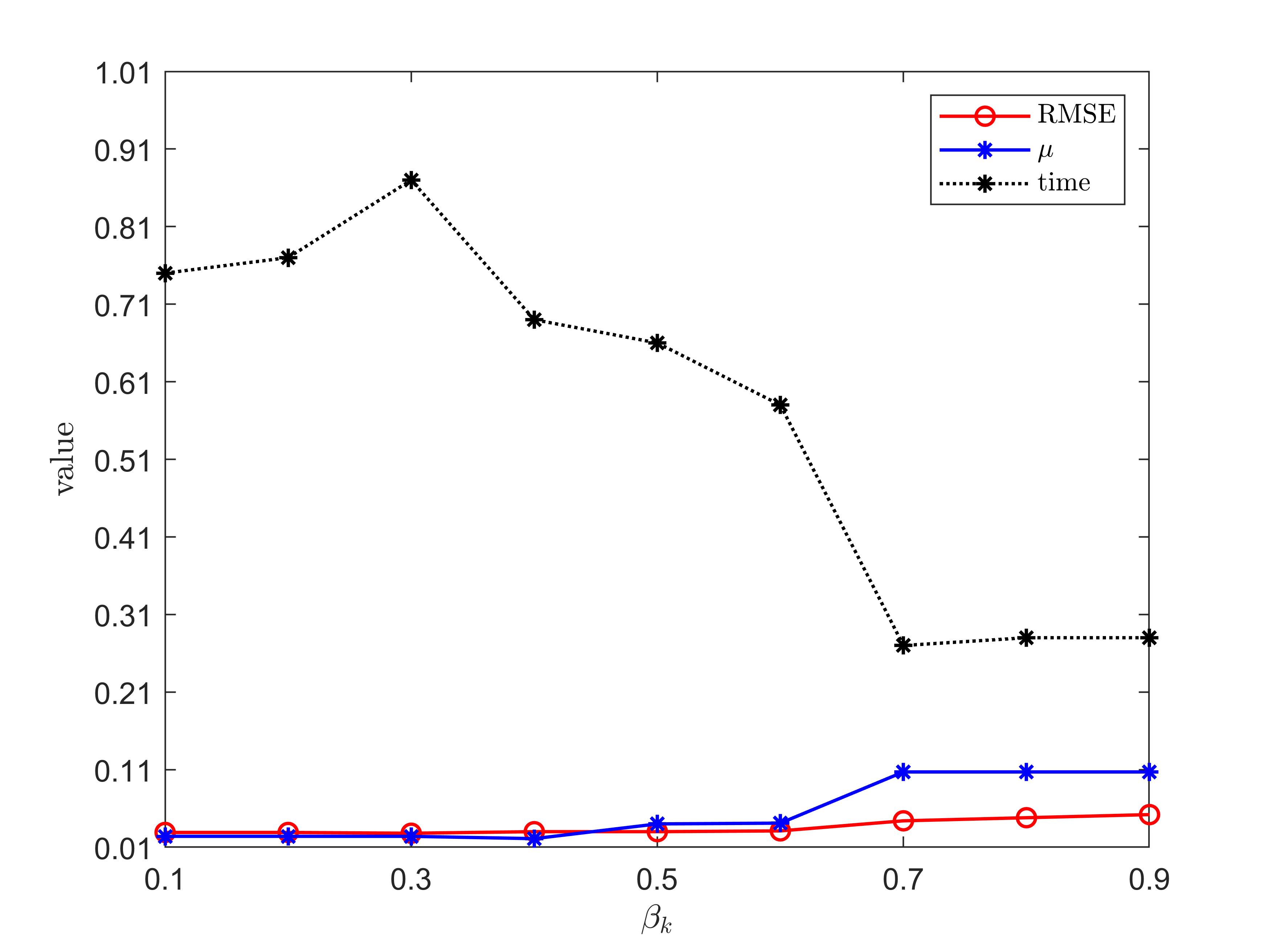
Moreover, in order to chose an appropriate value of , we perform the experiments to test the influence of different values of on GIMSPG algorithm from the RMSE, the last value of smoothing factor and . The details are presented in Figure 1. From it, we observe that the higher value of , the used time is less, but RMSE and the last value of the smoothing factor is larger. For the sake of balance, in the following experiments, we chose in Section 4.1 and 4.2. In Section 4.3, we chose .
4.1 Matrix completion on the random data
In this subsetion, we perform the numerical experiments on random generated data. In order to make a fair comparison, our results are averaged over 20 independent tests. Besides, the way of the generated data is same as Yu_Q_Zhang_X , in detail, we first randomly generate matrices and with i.i.d. standard Gaussian entries and let . We then sample a subset with sample ration uniformly at random, where . In the following experiments, the parameters in the GMM noise are set as . The rank of the matrix is set as and the sampling ration are given three different cases . The size of the square matrix increases from 100 to 200 with increament 10.
The root-mean-square error (RMSE) is defined as an error estimation criterion,
| (44) |
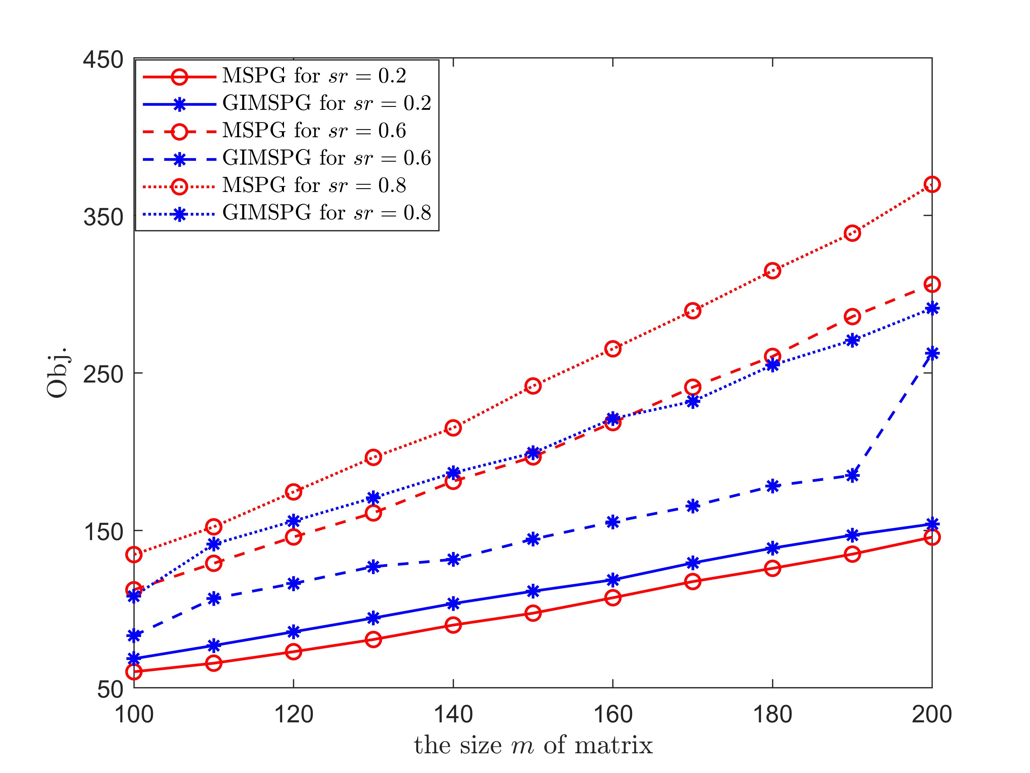
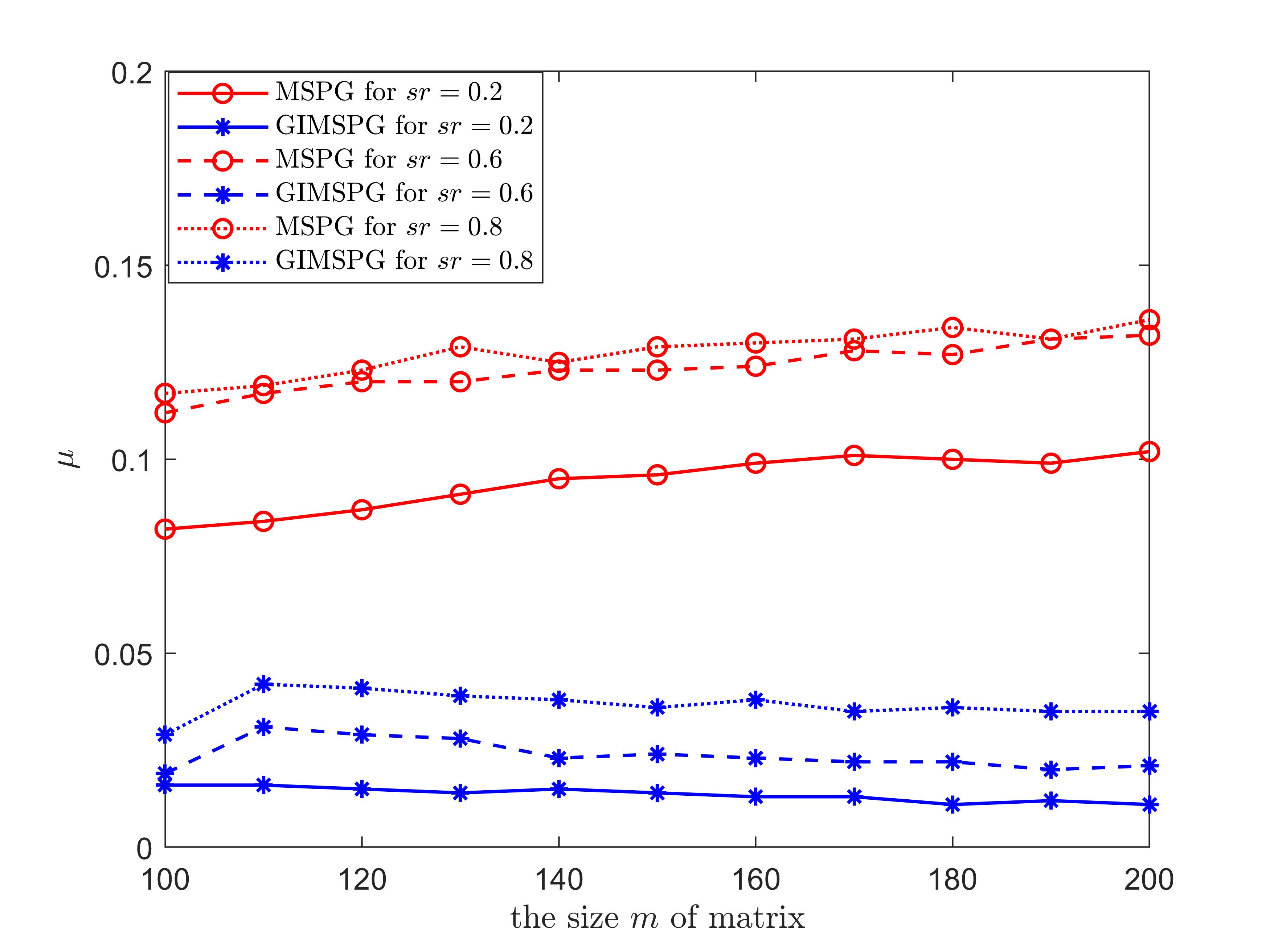
The Figure 2 presents the last value of the objective function and the last value of smoothing factor for GIMSPG algorithm and MSPG algorithm under different matrix size and . It can be easily seen that the last value of the objective function value of GIMSPG algorithm is lower than the MSPG algorithm except . Besides, the last value of smoothing factor of GIMSPG algorithm are far lower than the MSPG algorithm, that is, the model in GIMSPG algorithm can be better approxiamtion to the original problem. Moreover, we illustrate the efficiency of GIMSPG algorithm compared with MSPG, FPCA, SVT and VBMFL1 from RMSE and the running time two aspects under different matrix size for in Tabels 1,2,3. From them, we see that the running time of GIMSPG algorithm is the least one in these algorithms. We also observe that as the dimension increases, so does the time. Compared with MSPG algorithm, when the sample ratio is lower, the RMSE of GIMSPG algorithm is better. And compared with the other algorithms, the GIMSPG algorithm always has the least value of RMSE.
| RMSE | ||||||||||
|---|---|---|---|---|---|---|---|---|---|---|
| GIMSPG | MSPG | VBMFL1 | FPCA | SVT | GIMSPG | MSPG | VBMFL1 | FPCA | SVT | |
| 100 | 0.030 | 0.031 | 0.051 | 0.551 | 0.242 | 0.32 | 1.01 | 3.33 | 5.13 | 3.70 |
| 110 | 0.029 | 0.030 | 0.045 | 0.472 | 0.076 | 0.33 | 1.21 | 3.53 | 4.97 | 4.03 |
| 120 | 0.029 | 0.029 | 0.038 | 0.352 | 0.049 | 0.33 | 1.26 | 3.56 | 5.55 | 4.31 |
| 130 | 0.028 | 0.029 | 0.036 | 0.289 | 0.036 | 0.45 | 1.46 | 3.84 | 6.44 | 4.32 |
| 140 | 0.028 | 0.028 | 0.035 | 0.284 | 0.028 | 0.51 | 1.78 | 3.56 | 6.72 | 4.51 |
| 150 | 0.028 | 0.028 | 0.034 | 0.271 | 0.026 | 0.55 | 1.85 | 3.58 | 6.72 | 4.75 |
| 160 | 0.028 | 0.028 | 0.037 | 0.271 | 0.023 | 0.62 | 2.21 | 4.06 | 7.74 | 4.52 |
| 170 | 0.028 | 0.027 | 0.034 | 0.230 | 0.022 | 0.78 | 2.66 | 4.30 | 8.28 | 4.70 |
| 180 | 0.027 | 0.026 | 0.032 | 0.209 | 0.022 | 0.84 | 2.89 | 4.16 | 8.86 | 4.41 |
| 190 | 0.025 | 0.026 | 0.031 | 0.201 | 0.021 | 0.90 | 3.19 | 4.59 | 9.72 | 4.31 |
| 200 | 0.025 | 0.025 | 0.030 | 0.196 | 0.020 | 1.04 | 3.47 | 4.94 | 10.03 | 4.84 |
| RMSE | ||||||||||
|---|---|---|---|---|---|---|---|---|---|---|
| GIMSPG | MSPG | VBMFL1 | FPCA | SVT | GIMSPG | MSPG | VBMFL1 | FPCA | SVT | |
| 100 | 0.036 | 0.036 | 0.124 | 1.640 | 1.860 | 0.42 | 1.40 | 5.11 | 4.71 | 5.23 |
| 110 | 0.033 | 0.033 | 0.080 | 1.360 | 1.380 | 0.57 | 1.50 | 5.19 | 5.09 | 4.84 |
| 120 | 0.033 | 0.033 | 0.062 | 0.870 | 1.324 | 0.85 | 1.70 | 5.38 | 5.94 | 5.70 |
| 130 | 0.031 | 0.031 | 0.054 | 0.610 | 0.972 | 0.91 | 1.88 | 5.44 | 6.05 | 8.41 |
| 140 | 0.030 | 0.031 | 0.051 | 0.500 | 0.707 | 1.09 | 2.10 | 5.52 | 6.67 | 7.27 |
| 150 | 0.029 | 0.029 | 0.047 | 0.437 | 0.552 | 1.87 | 2.32 | 6.21 | 7.17 | 7.47 |
| 160 | 0.028 | 0.028 | 0.042 | 0.396 | 0.368 | 1.90 | 2.41 | 6.36 | 8.09 | 8.55 |
| 170 | 0.027 | 0.028 | 0.041 | 0.357 | 0.219 | 1.99 | 2.99 | 6.59 | 8.64 | 9.01 |
| 180 | 0.027 | 0.027 | 0.038 | 0.326 | 0.163 | 0.84 | 3.10 | 7.16 | 10.06 | 9.03 |
| 190 | 0.026 | 0.027 | 0.035 | 0.310 | 0.127 | 2.14 | 4.11 | 7.51 | 10.23 | 10.06 |
| 200 | 0.026 | 0.027 | 0.034 | 0.289 | 0.068 | 2.38 | 4.37 | 8.14 | 10.55 | 10.84 |
| RMSE | ||||||||||
|---|---|---|---|---|---|---|---|---|---|---|
| GIMSPG | MSPG | VBMFL1 | FPCA | SVT | GIMSPG | MSPG | VBMFL1 | FPCA | SVT | |
| 100 | 0.070 | 0.075 | 5.649 | 5.770 | 6.536 | 0.69 | 1.40 | 13.42 | 2.38 | 8.17 |
| 110 | 0.071 | 0.074 | 5.496 | 5.660 | 6.497 | 0.80 | 1.50 | 16.59 | 2.64 | 995 |
| 120 | 0.069 | 0.073 | 5.486 | 5.540 | 6.563 | 0.94 | 1.60 | 17.38 | 3.27 | 10.41 |
| 130 | 0.066 | 0.073 | 5.456 | 5.300 | 6.618 | 1.08 | 1.70 | 18.33 | 3.27 | 13.51 |
| 140 | 0.066 | 0.075 | 5.446 | 5.209 | 6.255 | 1.50 | 1.98 | 20.84 | 3.73 | 15.41 |
| 150 | 0.066 | 0.072 | 5.442 | 5.270 | 6.230 | 1.66 | 2.19 | 21.84 | 4.06 | 15.84 |
| 160 | 0.065 | 0.071 | 5.508 | 5.230 | 6.210 | 1.80 | 2.57 | 25.67 | 3.99 | 27.09 |
| 170 | 0.065 | 0.068 | 5.309 | 5.050 | 6.194 | 2.30 | 2.80 | 26.77 | 4.31 | 23.89 |
| 180 | 0.064 | 0.069 | 5.212 | 5.010 | 5.984 | 2.60 | 3.39 | 29.16 | 5.25 | 29.01 |
| 190 | 0.062 | 0.068 | 5.091 | 4.970 | 5.020 | 2.63 | 3.58 | 29.98 | 5.98 | 29.21 |
| 200 | 0.062 | 0.067 | 4.239 | 4.680 | 5.064 | 3.20 | 4.82 | 32.83 | 6.66 | 29.77 |
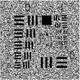
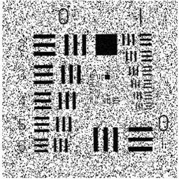
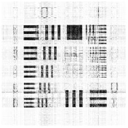
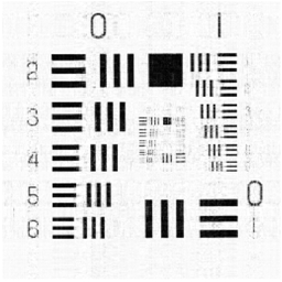
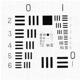
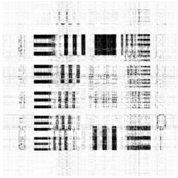
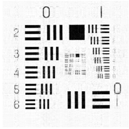
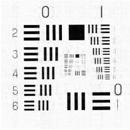
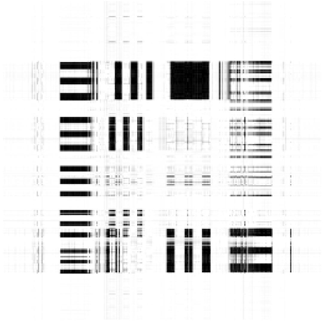
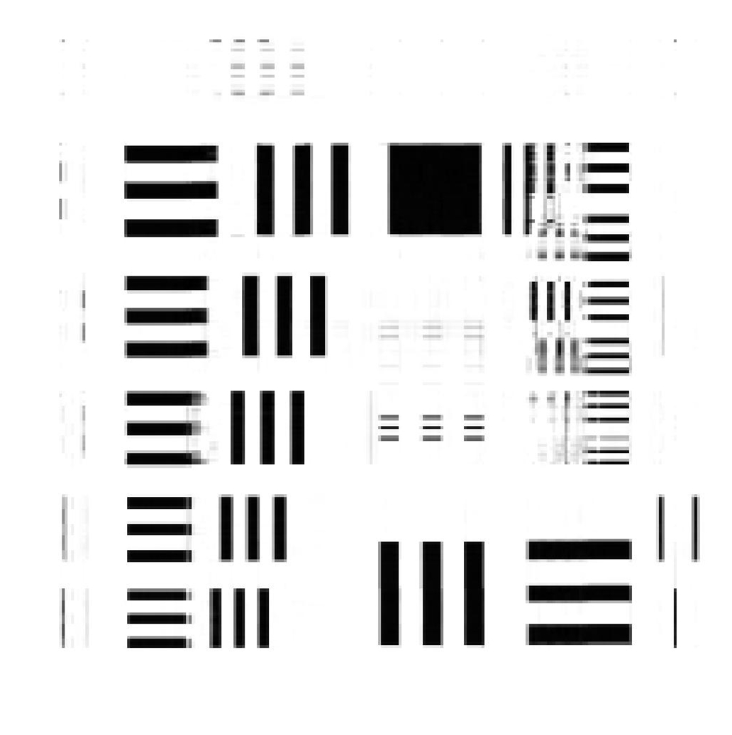
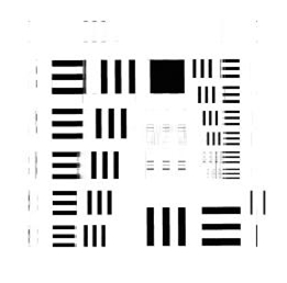
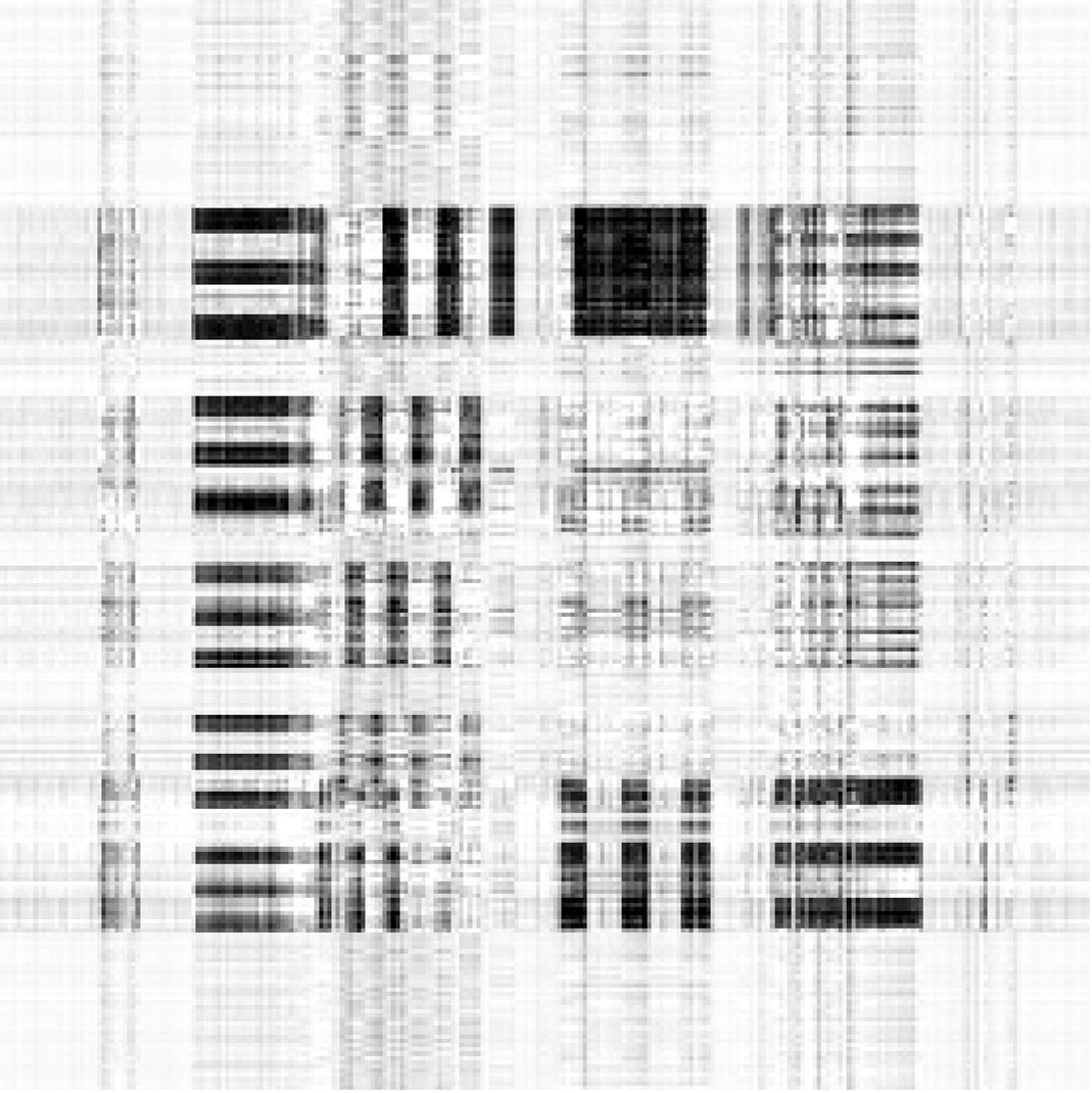
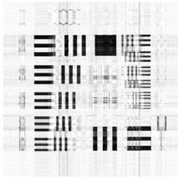
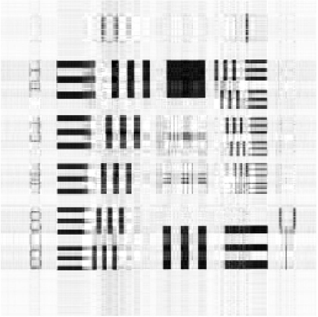
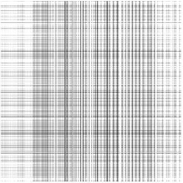
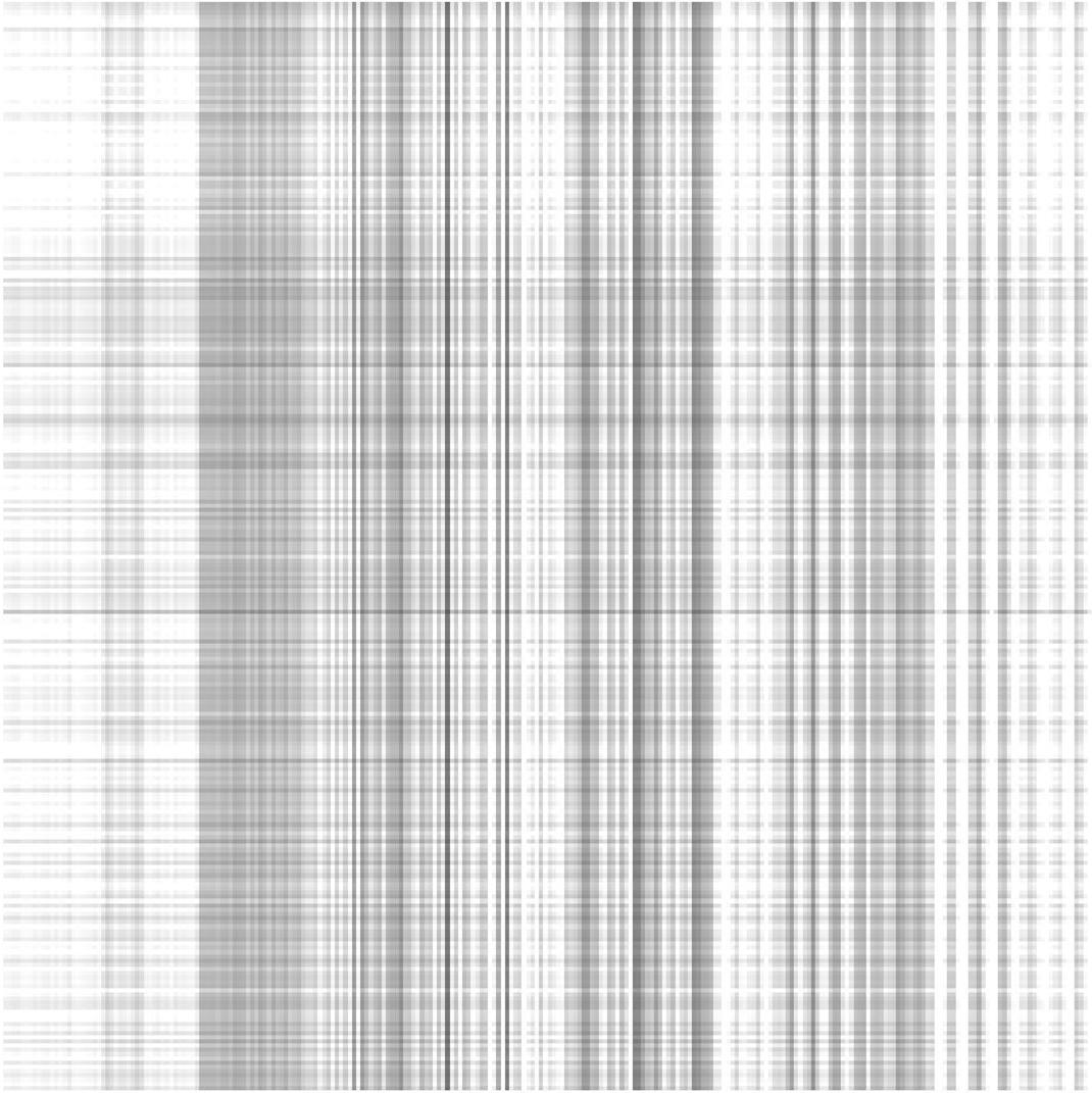
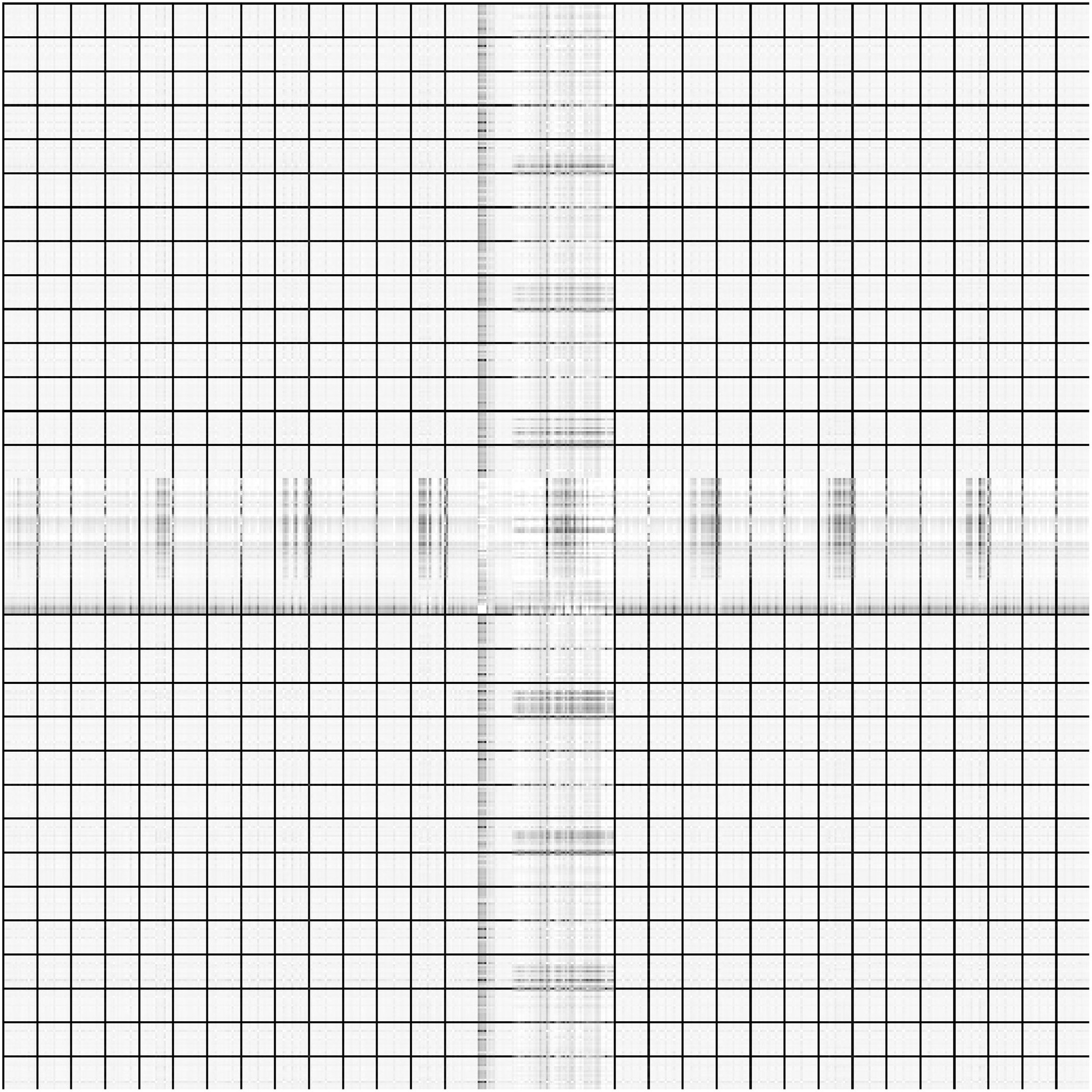
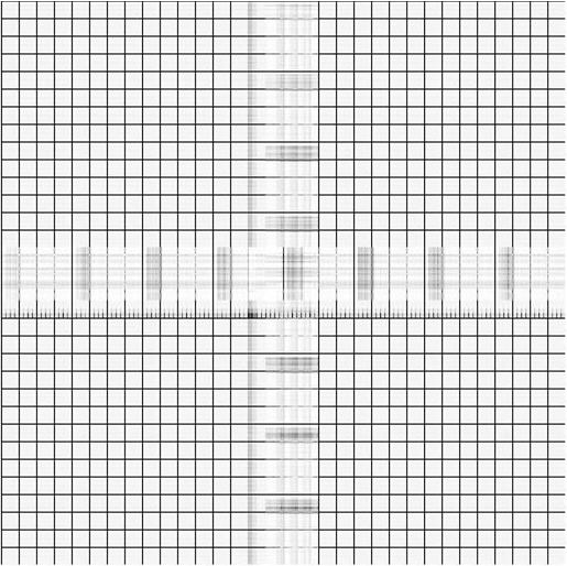
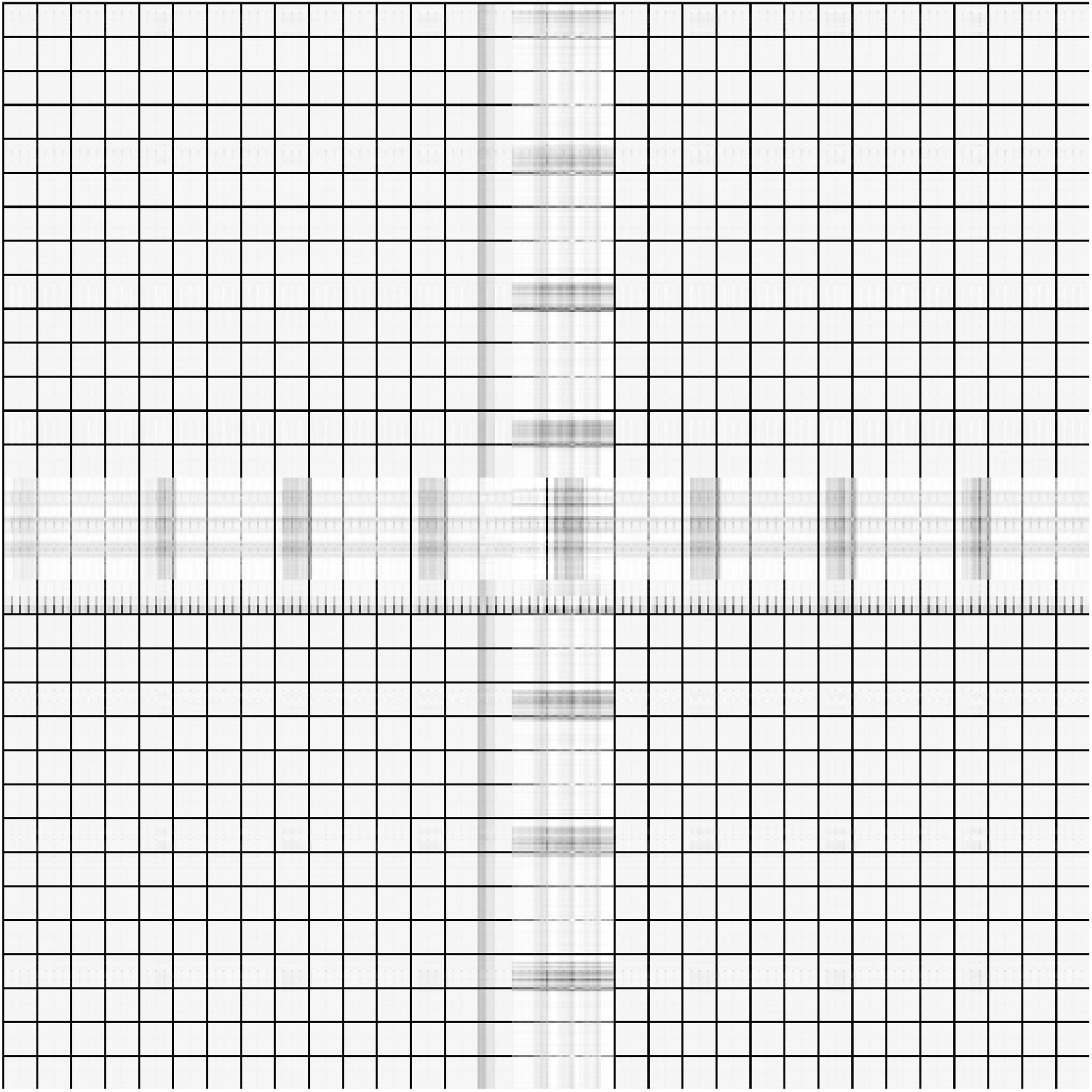
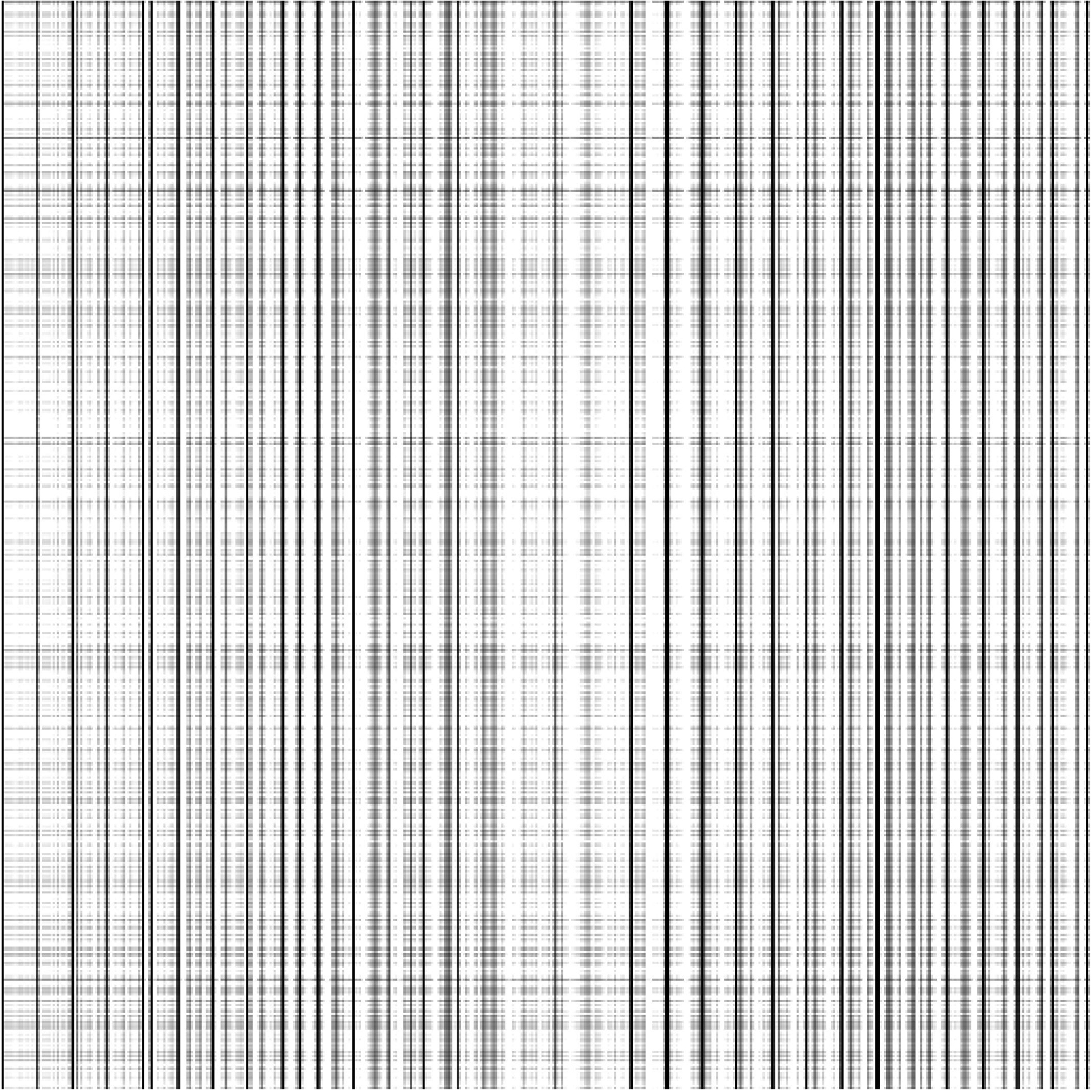
4.2 Image inpainting
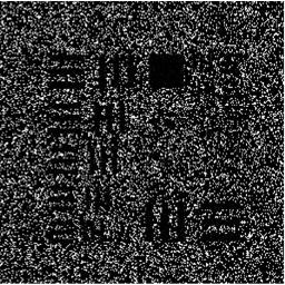
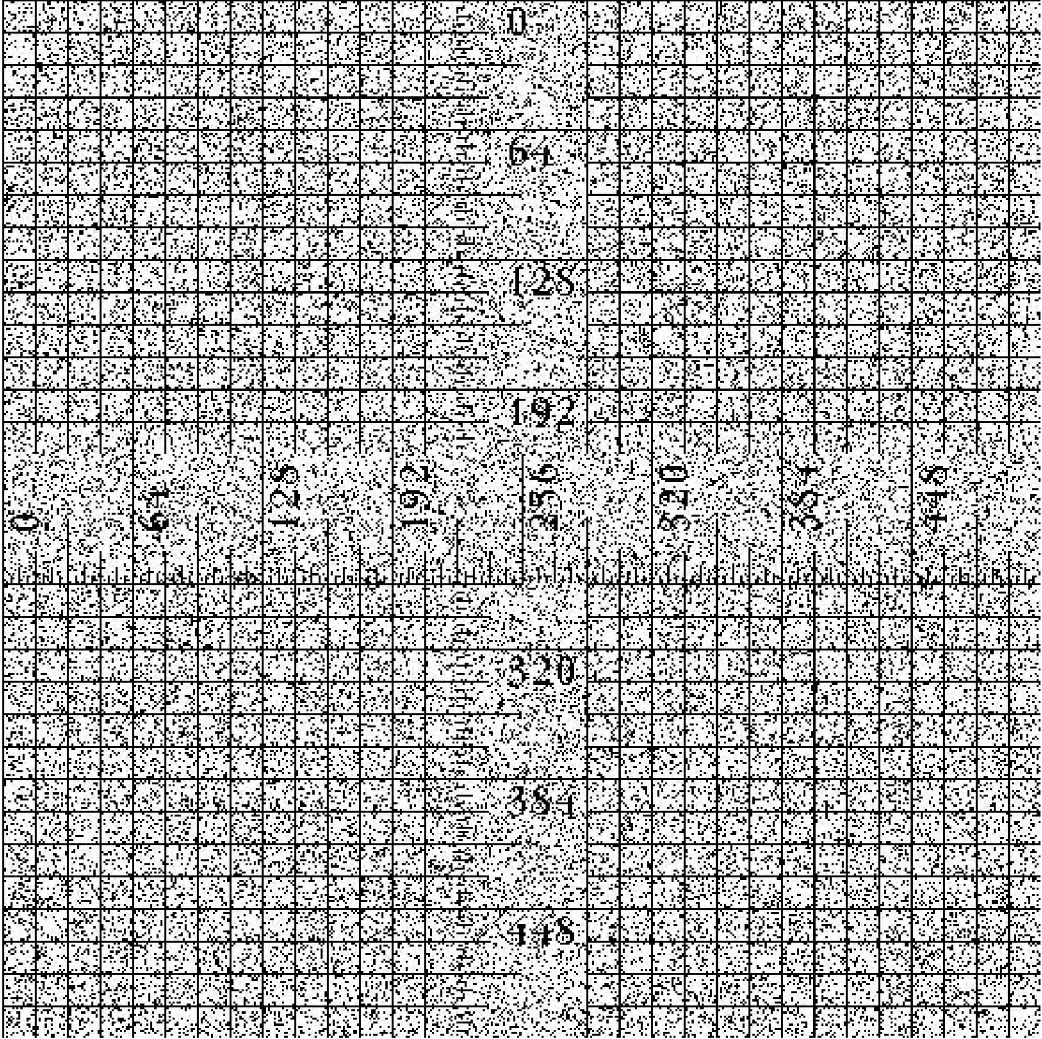
In this subsection, we aim to illustrate the efficiency of GIMSPG algorithm by solving a grayscale inpainting problem with non-Gaussian noise. The image inpainting problem is to fill the missing pixel values of the image at given pixel locations. In fact, the grayscale image can be seen as the matrix, and the image inpainting problem can be represented as the matrix completion problem if the matrix satisfies the property of the low rank. In our experiments, two different grayscale images are considered which are from the USC-SIPI image database 111http://sipi.usc.edu/database/.. In detail, they are “Chart” and “Ruler". “Chart” is an image with pixels and rank . “Ruler” is an image with with rank . To evaluate the performance of the GIMSPG algorithm under the non-Gaussian noise, the peak signal-to-noise ratio (PSNR) is considered as an evaluation metric which is defined as follows:
We solve the image inpainting problem under three different sample ratios . From the results in Table 5, we observe that the last value of smoothing factor of GIMSPG algorithm is less than MSPG algorithm in each case. The used time of GIMSPG is the least in these algorithms. The PSNR of GIMSPG algorithm is higher than MSPG for and obviously higher than algorithm in all the cases. From Figures 3, 4, one can see that the recoverability of GIMSPG algorithm is slightly better than that MSPG algorithm espeically in the lower sample rate and apparently better than others.

| Image | sr | PSNR | T | ||||||||||
|---|---|---|---|---|---|---|---|---|---|---|---|---|---|
| GIMSPG | MSPG | VBMFL1 | FPCA | SVT | GIMSPG | MSPG | VBMFL1 | FPCA | SVT | MSPGE | MSPG | ||
| chart | 0.2 | 18.04 | 17.16 | 15.96 | 15.60 | 9.16 | 9.78 | 18.10 | 18.67 | 0.53 | 2.72 | 0.022 | 0.062 |
| 0.6 | 29.13 | 29.01 | 19.80 | 18.80 | 10.49 | 2.19 | 12.59 | 33.10 | 14.16 | 2.78 | 0.035 | 0.131 | |
| 0.8 | 30.84 | 30.18 | 20.63 | 19.50 | 10.65 | 1.55 | 3.16 | 47.94 | 13.64 | 3.58 | 0.107 | 0.234 | |
| ruler | 0.2 | 21.17 | 20.74 | 20.10 | 19.90 | 5.21 | 25.45 | 55.76 | 5.23 | 26.25 | 5.42 | 0.020 | 0.105 |
| 0.6 | 27.02 | 27.04 | 19.80 | 18.80 | 5.22 | 11.50 | 12.86 | 19.67 | 54.91 | 6.31 | 0.044 | 0.238 | |
| 0.8 | 30.01 | 30.39 | 20.50 | 20.20 | 5.24 | 7.11 | 14.83 | 49.91 | 49.98 | 7.09 | 0.093 | 0.273 | |
| \botrule | |||||||||||||
| Image | sr | PSNR | T | ||||||||||
|---|---|---|---|---|---|---|---|---|---|---|---|---|---|
| GIMSPG | MSPG | VBMFL1 | FPCA | SVT | GIMSPG | MSPG | VBMFL1 | FPCA | SVT | MSPGE | MSPG | ||
| MRI | 0.6 | 29.13 | 29.01 | 29.58 | 26.70 | 13.56 | 2.19 | 12.59 | 32.91 | 10.67 | 2.22 | 0.035 | 0.131 |
| 0.8 | 33.06 | 32.99 | 30.33 | 27.20 | 13.59 | 1.79 | 10.57 | 26.61 | 11.58 | 2.44 | 0.029 | 0.137 | |
| \botrule | |||||||||||||
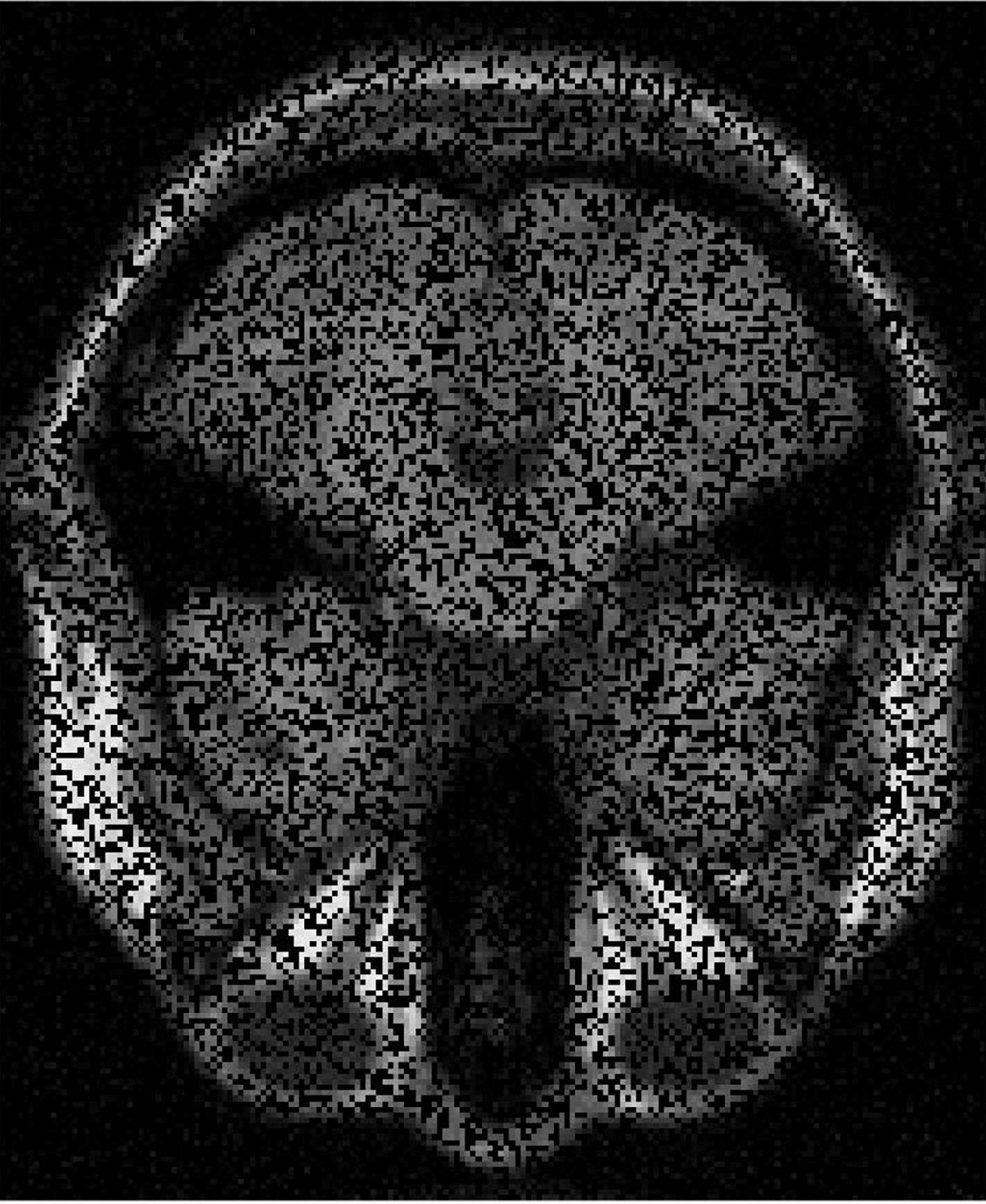
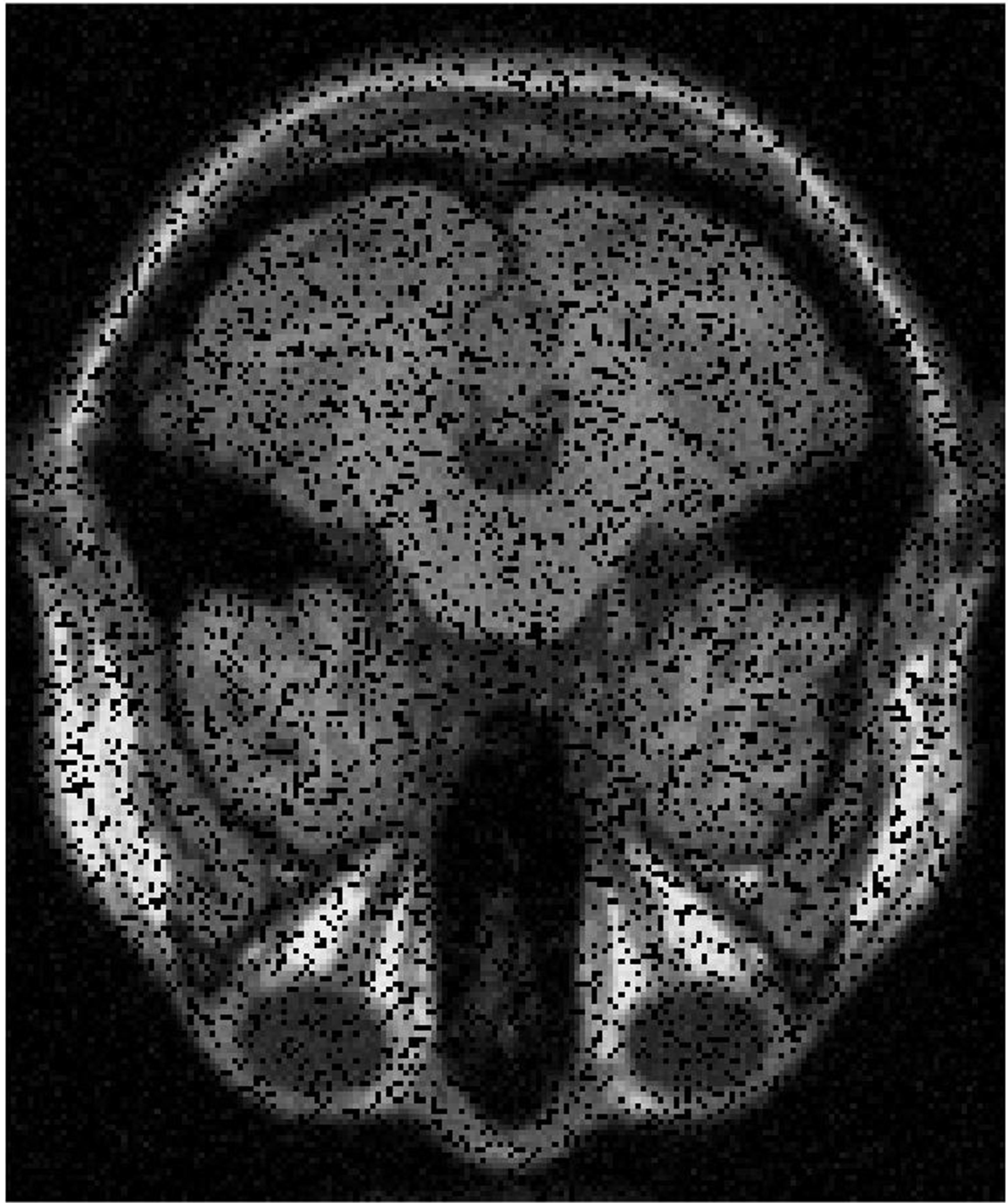
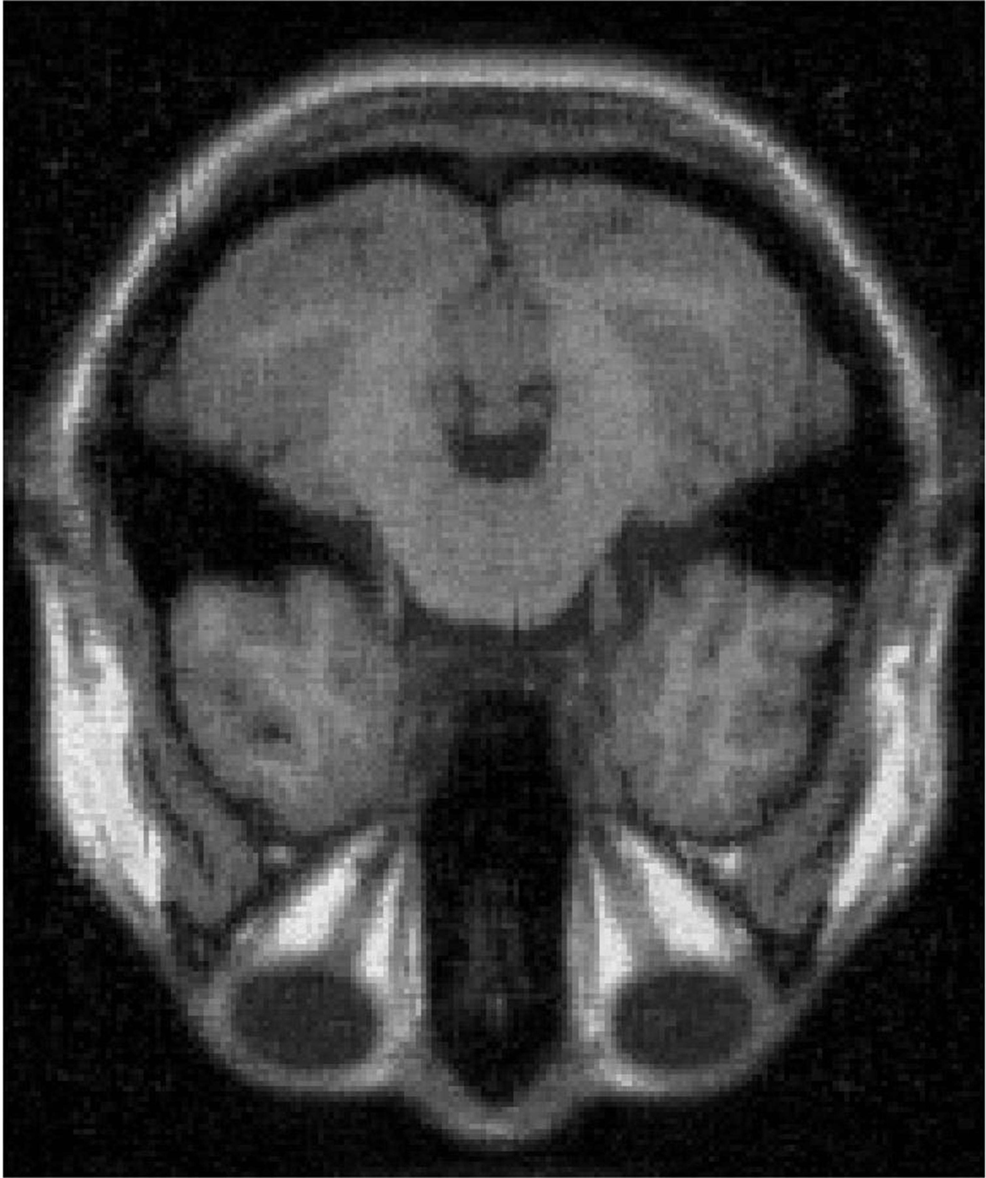
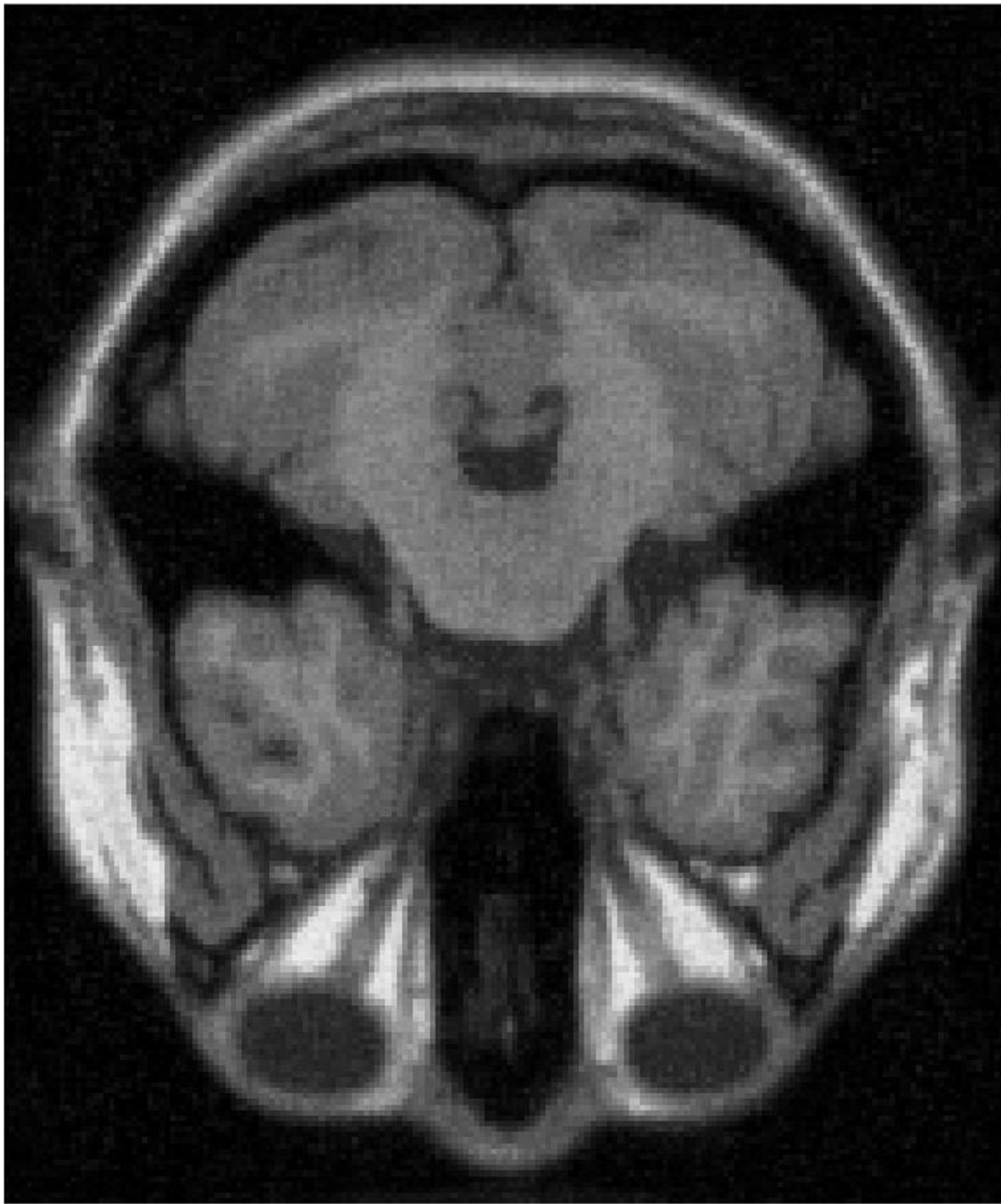
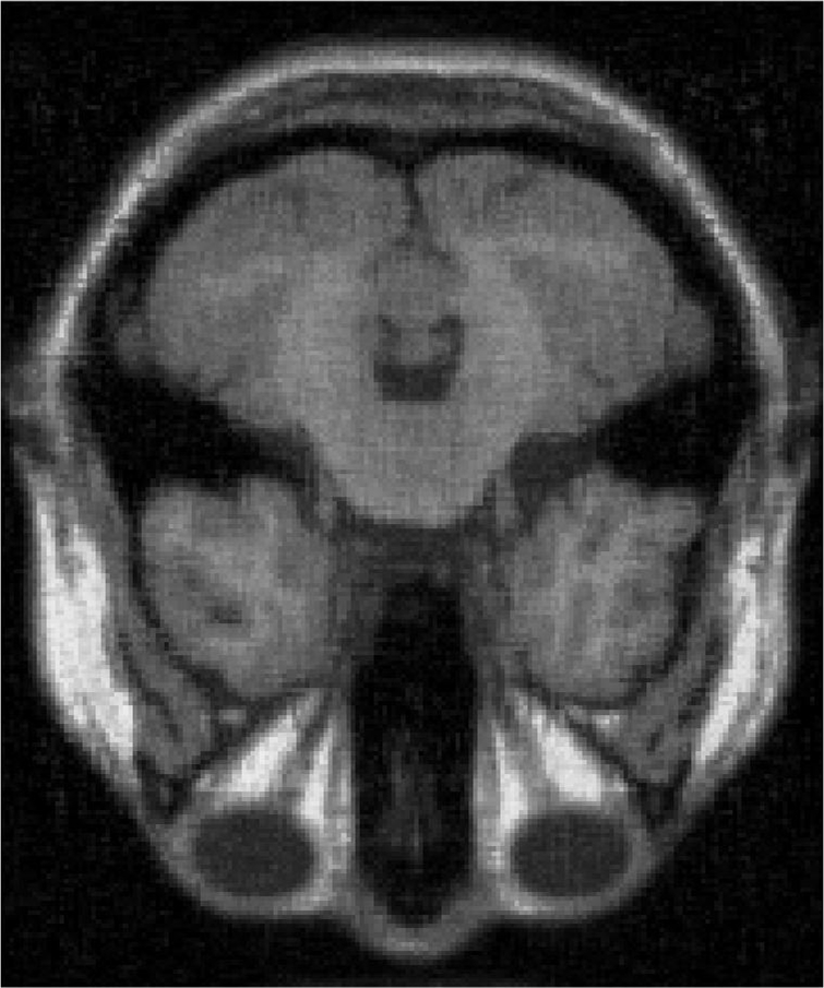
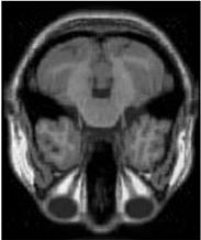
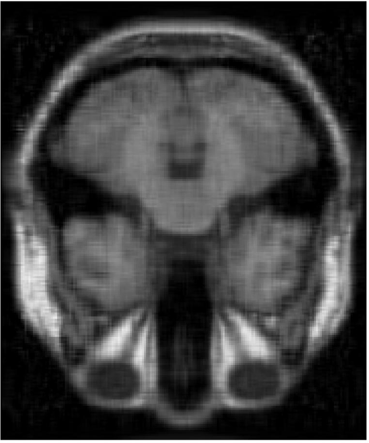
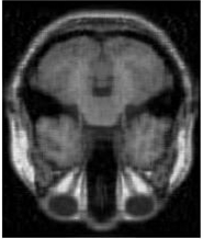
4.3 MRI Volume Dataset
In this subsection, we perform the experiments on the MRI image which is of size with 181 slices and we select the 38th slice for the experiments. The two sampling ratios are considered. The parameters in GMM noise are set as , and .
From Figure 5 and Table 5, we see that the recoverability of VBMFL1 is relatively better but it spends more time. Particularly, we notice that the PSNR of GIMSPG algorithm is higher than other algorithms except the VBMFL1 in Table 5. Besides, the used time of GIMSPG is the least one. Compared with MSPG, the last value of smoothing facor of GIMSPG algorithm is lower.


5 Conclusions
This paper mainly proposes the GIMSPG algorithm for the exact continuous model Yu_Q_Zhang_X of matrix rank minimization problem and discuss its convergence under the flexible parameters condition. It is shown that the singular values of the accumulation point have a common support set and the nonzero elements have a unified lower bound. Further, the zero singular values of the accumulation point can be achieved within finite iterations. Moreover, we prove that any accumulation point of the sequence generated by GIMSPG algorithm is a lifted stationary point of the continuous relaxation model under the flexible parameter constraint. Further, we generalize Euclidean distance to the Bregman distance in the GIMSPG algorithm and the . Under the appropriate parameters, the range of the extrapolation parameters is large enough which also includes the sFISTA system (1) with fixted restart. At last, the superiority of the GIMSPG algorithm is verified on random data and real image data respectively.
Appendix A Appendix
Lemma 6.
For any , suppose be the sequence generated by GIMSPG, we have
When the parameters satisfying Assumption 5, it holds that
| (45) |
Moreover, the sequence is a nonincreasing sequence.
Proof: By (40), we have
| (46) |
Since has Lipschitz constant , it follows from the Definition 2(v) that
| (47) |
Moreover, is convex with respect to , we have
| (48) |
Combining (A), (47) and (48), we have
| (49) | ||||
Denote , then it has , , . That is,
| (50) |
where the second inequality comes from the Cauchy-Schwartz inequality.
References
- (1) Argyriou, A., Evgeniou, T., Pontil, M.: Convex multi-task feature learning. Mach. Learn. 73, 243-272 (2008)
- (2) Beck, A., Teboulle, M.: A fast iterative shrinkage-thresholding algorithm for linear inverse problems. SIAM J. Imaging Sci. 2, 183-202 (2009)
- (3) Bian,W.: Smoothing accelerated algorithm for constrained nonsmooth convex optimization problems (in Chinese). Sci. Sin. Math. 50, 1651–1666 (2020)
- (4) Bolte, J., Sabach, S., Teboulle, M., Vaisbourd, Y.: First-order methods beyond convexity and Lipschitz gradient continuity with applications to quadratic inverse problems. SIAM J. Optim. 28, 2131-2151 (2018)
- (5) Bian, W., Chen, X.: A smoothing proximal gradient algorithm for nonsmooth convex regression with cardinality penalty. SIAM J. Numer. Anal. 58, 858-883 (2020)
- (6) Bouwmans,T., Zahzah, E, H.: Robust PCA via Principal Component Pursuit: A Review for a Comparative Evaluation in Video Surveillance. Comput Vis. Image Underst. 122, 22-34 (2014)
- (7) Cai, J., Candes, E., Shen, Z.: A singular value thresholding algorithm for matrix completion. SIAM J. Optim. 20, 1956-1982 (2008)
- (8) Chambolle, A., Dossal, C.: On the convergence of the iterates of the “fast iterative shrinkage/thresholding algorithm". J. Optim. Theory Appl. 166, 968-982 (2015)
- (9) Chen, X.: Smoothing methods for nonsmooth, nonconvex minimization. Math. Program. 134, 71-99 (2012)
- (10) Fornasier, M., Rauhut, H., Ward, R.: Low-rank matrix recovery via iteratively reweighted least squares minimization. SIAM J. Optim. 21, 1614-1640 (2011)
- (11) He, Y., Wang, F., Li, Y., Qin, J., Chen, B.: Robust matrix completion via maximum correntropy criterion and half-quadratic optimization. IEEE T. Signal Proces. 68, 181-195 (2020)
- (12) Ji, S., Ye, J.: An accelerated gradient method for trace norm minimization. Proceedings of the 26th annual international conference on machine learning. 457-464 (2009)
- (13) Kulis, B., Sustik, M.,A., Dhillon, I.,S.: Low-Rank Kernel Learning with Bregman Matrix Divergences. J. Mach. Learn. Res. 10, 2009
- (14) Lai, M., Xu,Y., Yin, W.: Improved iteratively reweighted least squares for unconstrained smoothed q minimization. SIAM J. Numer. Anal. 51, 927-957 (2013)
- (15) Lewis, A, S., Sendov, H, S.: Nonsmooth analysis of singular values. Part II: Applications. Set-Valued Anal. 13, 243-264 (2005)
- (16) Li, W., Bian, W., Toh, K, C.: DC algorithms for a class of sparse group regularized optimization problems (2021). arXiv:2109.05251
- (17) Liang, J., Schonlieb, C, B.: “Faster FISTA." European Signal Processing Conference. (2018)
- (18) Lu, Z., Zhang, Y., Lu, J.: Regularized low-rank approximation via iterative reweighted singular value minimization. Comput. Optim. Appl. 68, 619-642 (2017)
- (19) Ma, S., Goldfarb, D., Chen, L.: Fixed point and Bregman iterative methods for matrix rank minimization. Math. Program. 128, 321-353 (2011)
- (20) Ma, T., H., Lou, Y., Huang, T., Z.: Truncated models for sparse recovery and rank minimization. SIAM J. Imaging Sci. 10, 1346-1380 (2017)
- (21) Mesbahi, M., Papavassilopoulos, G., P.: On the rank minimization problem over a positive semidefinite linear matrix inequality. IEEE T. Automat. Contr. 42, 239-243(1997)
- (22) Nesterov, Y.: Introductory Lectures on Convex Programming. Kluwer Academic Publisher, Dordrecht (2004)
- (23) Nesterov Y. Gradient methods for minimizing composite functions[J]. Mathematical programming, 2013, 140(1): 125-161.
- (24) Nesterov, Y.: A method for solving the convex programming problem with convergence rate . Dokl. Akad. Nauk. SSSR 269, 543¨C547 (1983)
- (25) O’Donoghue, B., Candes, E.J.: Adaptive restart for accelerated gradient schemes. Found. Comput. Math. 15, 715-732 (2015)
- (26) Parikh, N., Boyd, S.: Proximal algorithms. Found. Trends Mach. Learn. 1, 127-239 (2014)
- (27) Recht, B., Fazel, M., Parrilo, P.: Guaranteed minimum-rank solutions of linear matrix equations via nuclear norm minimization. Siam Rev. 52, 471-501 (2010)
- (28) Teboulle, M.: A simplified view of first order methods for optimization. Math. Program. 170, 67-96 (2018)
- (29) Toh, K., C., Yun, S.: An accelerated proximal gradient algorithm for nuclear norm regularized linear least squares problems. Pac. J. Optim. 6, 615-640 (2010)
- (30) Wu, F., Bian, W., Xue, X.: Smoothing fast iterative hard thresholding algorithm for regularized nonsmooth convex regression problem (2021). arXiv:2104.13107
- (31) Wu, Z., Li, C., Li, M., Lim, A.: Inertial proximal gradient methods with Bregman regularization for a class of nonconvex optimization problems. J. Global Optim. 79, 617-644 (2021)
- (32) Wu, Z., Li, M.: General inertial proximal gradient method for a class of nonconvex nonsmooth optimization problems. Comput. Optim. Appl. 73, 129-158(2019)
- (33) Xu, H., Caramanis, C., Sanghavi, S.: Robust PCA via outlier pursuit. IEEE Trans. Inf. Theory. 58, 3047-3064 (2012)
- (34) Yu, Q., Zhang, X.: A smoothing proximal gradient algorithm for matrix rank minimization problem. Comput. Optim. Appl. 1-20 (2022)
- (35) Zhang, C., Chen, X.: Smoothing projected gradient method and its application to stochastic linear complementarity problems. SIAM J. Optim. 20, 627-649(2009)
- (36) Zhang, J., Yang, X., Li, G., Zhang, K. The smoothing proximal gradient algorithm with extrapolation for the relaxation of regularization problem (2021). arXiv:2112.01114.
- (37) Zhao, Q., Meng, D., Xu, Z., Yan, Y.: -norm low-rank matrix factorization by variational Bayesian method. IEEE T. Neur. Net. Lear. 26, 825-839(2015)
- (38) Zheng, Y., Liu, G., Sugimoto, S., Yan, S., Okutomi, M.: Practical low-rank matrix approximation under robust -norm. In 2012 IEEE Conference on Computer Vision and Pattern Recognition (pp. 1410-1417). IEEE