Google, aigerd@google.com School of Computer Science, Tel Aviv University, Tel Aviv, and Googlehaimk@tau.ac.ilPartially supported by ISF grant 1841/14, by grant 1367/2016 from the German-Israeli Science Foundation (GIF), and by Blavatnik Research Fund in Computer Science at Tel Aviv University.Google, efi@google.com School of Computer Science, Tel Aviv University, Tel Aviv, Israelmichas@tau.ac.ilPartially supported by ISF Grant 260/18, by grant 1367/2016 from the German-Israeli Science Foundation (GIF), and by Blavatnik Research Fund in Computer Science at Tel Aviv University. Google, bzeisl@google.com \CopyrightD. Aiger, H. Kaplan, E. Kokiopoulou, M. Sharir, B. Zeisl \EventEditors \EventNoEds2 \EventLongTitle \EventShortTitle \EventAcronym \EventYear \EventDate \EventLocation \EventLogo \SeriesVolume \ArticleNo
General techniques for approximate incidences and their application to the camera posing problem
Abstract.
We consider the classical camera pose estimation problem that arises in many computer vision applications, in which we are given 2D-3D correspondences between points in the scene and points in the camera image (some of which are incorrect associations), and where we aim to determine the camera pose (the position and orientation of the camera in the scene) from this data. We demonstrate that this posing problem can be reduced to the problem of computing -approximate incidences between two-dimensional surfaces (derived from the input correspondences) and points (on a grid) in a four-dimensional pose space. Similar reductions can be applied to other camera pose problems, as well as to similar problems in related application areas.
We describe and analyze three techniques for solving the resulting -approximate incidences problem in the context of our camera posing application. The first is a straightforward assignment of surfaces to the cells of a grid (of side-length ) that they intersect. The second is a variant of a primal-dual technique, recently introduced by a subset of the authors [2] for different (and simpler) applications. The third is a non-trivial generalization of a data structure Fonseca and Mount [3], originally designed for the case of hyperplanes. We present and analyze this technique in full generality, and then apply it to the camera posing problem at hand.
We compare our methods experimentally on real and synthetic data. Our experiments show that for the typical values of and , the primal-dual method is the fastest, also in practice.
Key words and phrases:
Camera positioning, Approximate incidences, Incidences1991 Mathematics Subject Classification:
F.2.2 Nonnumerical Algorithms and Problems1. Introduction
Camera pose estimation is a fundamental problem in computer vision, which aims at determining the pose and orientation of a camera solely from an image. This localization problem appears in many interesting real-world applications, such as for the navigation of self-driving cars [5], in incremental environment mapping such as Structure-from-Motion (SfM) [1, 11, 13], or for augmented reality [8, 9, 14], where a significant component are algorithms that aim to estimate an accurate camera pose in the world from image data.
Given a three-dimensional point-cloud model of a scene, the classical, but also state-of-the-art approach to absolute camera pose estimation consists of a two-step procedure. First, one matches a large number of features in the two-dimensional camera image with corresponding features in the three-dimensional scene. Then one uses these putative correspondences to determine the pose and orientation of the camera. Typically, the matches obtained in the first step contain many incorrect associations, forcing the second step to use filtering techniques to reject incorrect matches. Subsequently, the absolute 6 degrees-of-freedom (DoF) camera pose is estimated, for example, with a perspective -point pose solver [6] within a RANSAC scheme [4].
In this work we concentrate on the second step of the camera pose problem. That is, we consider the task of estimating the camera pose and orientation from a (potentially large) set of already calculated image-to-scene correspondences.
Further, we assume that we are given a common direction between the world and camera frames. For example, inertial sensors, available on any smart-phone nowadays, allow to estimate the vertical gravity direction in the three-dimensional camera coordinate system. This alignment of the vertical direction fixes two degrees of freedom for the rotation between the frames and we are left to estimate four degrees of freedom out of the general six. To obtain four equations (in the four remaining degrees of freedom), this setup requires two pairs of image-to-scene correspondences111As we will see later in detail, each correspondence imposes two constraints on the camera pose. for a minimal solver. Hence a corresponding naive RANSAC-based scheme requires filtering steps, where in each iterations a pose hypothesis based on a different pair of correspondences is computed and verified against all other correspondences.
Recently, Zeisl et al. [17] proposed a Hough-voting inspired outlier filtering and camera posing approach, which computes the camera pose up to an accuracy of from a set of D-D correspondences, in time, under the same alignment assumptions of the vertical direction. In this paper we propose new algorithms that work considerably faster in practice, but under milder assumptions. Our method is based on a reduction of the problem to a problem of counting -approximate incidences between points and surfaces, where a point is -approximately incident (or just -incident) to a surface if the (suitably defined) distance between and is at most . This notion has recently been introduced by a subset of the authors in [2], and applied in a variety of instances, involving somewhat simpler scenarios than the one considered here. Our approach enables us to compute a camera pose when the number of correspondences is large, and many of which are expected to be outliers. In contrast, a direct application of RANSAC-based methods on such inputs is very slow, since the fraction of inliers is small. In the limit, trying all pairs of matches involves RANSAC iterations. Moreover, our methods enhance the quality of the posing considerably [17], since each generated candidate pose is close to (i.e., consistent with) with many of the correspondences.
Our results. We formalize the four degree-of-freedom camera pose problem as an approximate incidences problem in Section 2. Each 2D-3D correspondence is represented as a two-dimensional surface in the 4-dimensional pose-space, which is the locus of all possible positions and orientations of the camera that fit the correspondence exactly. Ideally, we would like to find a point (a pose) that lies on as many surfaces as possible, but since we expect the data to be noisy, and the exact problem is inefficient to solve anyway, we settle for an approximate version, in which we seek a point with a large number of approximate incidences with the surfaces.
Formally, we solve the following problem. We have an error parameter , we lay down a grid on of side length , and compute, for each vertex of the grid, a count of surfaces that are approximately incident to , so that (i) every surface that is -incident to is counted in , and (ii) every surface that is counted in is -incident to , for some small constant (but not all -incident surfaces are necessarily counted). We output the grid vertex with the largest count (or a list of vertices with the highest counts, if so desired).
As we will comment later, (a) restricting the algorithm to grid vertices only does not miss a good pose : a vertex of the grid cell containing serves as a good substitute for , and (b) we have no real control on the value of , which might be much larger than the number of surfaces that are -incident to , but all the surfaces that we count are ‘good’—they are reasonably close to . In the computer vision application, and in many related applications, neither of these issues is significant.
We give three algorithms for this camera-pose approximate-incidences problem. The first algorithm simply computes the grid cells that each surface intersects, and considers the number of intersecting surfaces per cell as its approximate -incidences count. This method takes time for all vertices of our -size grid. We then describe a faster algorithm using geometric duality, in Section 3. It uses a coarser grid in the primal space and switches to a dual 5-dimensional space (a 5-tuple is needed to specify a D-D correspondence and its surface, now dualized to a point). In the dual space each query (i.e., a vertex of the grid) becomes a 3-dimensional surface, and each original 2-dimensional surface in the primal 4-dimensional space becomes a point. This algorithm takes time, and is asymptotically faster than the simple algorithm for .
Finally, we give a general method for constructing an approximate incidences data structure for general -dimensional algebraic surfaces (that satisfy certain mild conditions) in , in Section 4. It extends the technique of Fonseca and Mount [3], designed for the case of hyperplanes, and takes time, where the degree of the polynomial in depends on the number of parameters needed to specify a surface, the dimension of the surfaces, and the dimension of the ambient space. We first present and analyze this technique in full generality, and then apply it to the surfaces obtained for our camera posing problem. In this case, the data structure requires storage and is constructed in roughly the same time. This is asymptotically faster than our primal-dual scheme when (for the term dominates and these two methods are asymptotically the same). Due to its generality, the latter technique is easily adapted to other surfaces and thus is of general interest and potential. In contrast, the primal-dual method requires nontrivial adaptation as it switches from one approximate-incidences problem to another and the dual space and its distance function depend on the type of the input surfaces.
We implemented our algorithms and compared their performance on real and synthetic data. Our experimentation shows that, for commonly used values of and in practical scenarios (, ), the primal-dual scheme is considerably faster than the other algorithms, and should thus be the method of choice. Due to lack of space, the experimentation details are omitted in this version, with the exception of a few highlights. They can be found in the appendix.
2. From camera positioning to approximate incidences
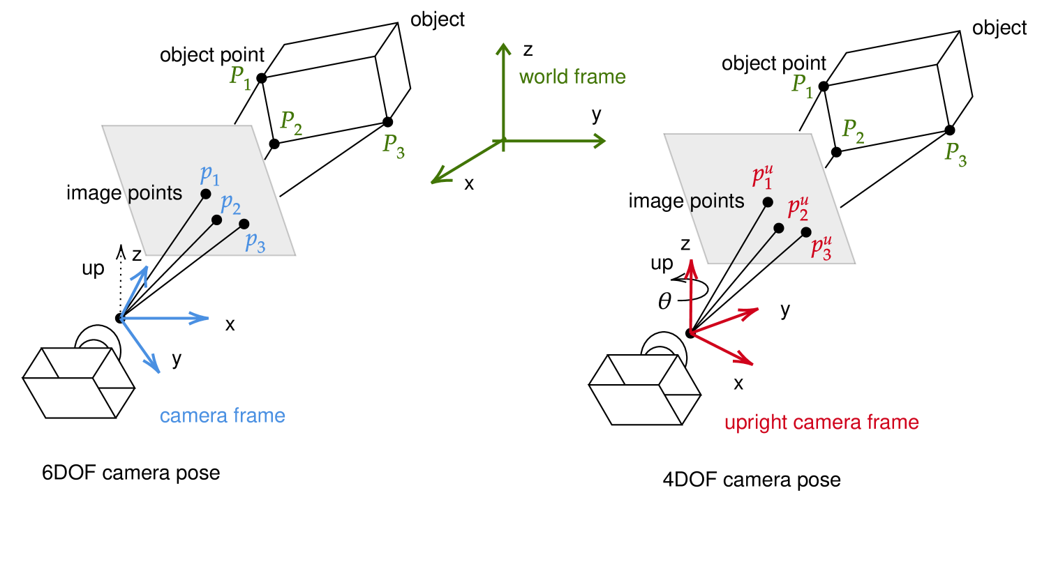
Suppose we are given a pre-computed three-dimensional scene and a two-dimensional picture of it. Our goal is to deduce from this image the location and orientation of the camera in the scene. In general, the camera, as a rigid body in 3-space, has six degrees of freedom, three of translation and three of rotation (commonly referred to as the yaw, pitch and roll). We simplify the problem by making the realistic assumption, that the vertical direction of the scene is known in the camera coordinate frame (e.g., estimated by en inertial sensor on smart phones). This allows us to rotate the camera coordinate frame such that its -axis is parallel to the world -axis, thereby fixing the pitch and roll of the camera and leaving only four degrees of freedom , where is the location of the camera center, say, and is its yaw, i.e. horizontal the orientation of the optical axis around the vertical direction. See Figure 1.
By preprocessing the scene, we record the spatial coordinates of a discrete (large) set of salient points. We assume that some (ideally a large number) of the distinguished points are identified in the camera image, resulting in a set of image-to-scene correspondences. Each correspondence is parameterized by five parameters, the spatial position and the position in the camera plane of view of the same salient point. Our goal is to find a camera pose so that as many correspondences as possible are (approximately) consistent with it, i.e., the ray from the camera center to goes approximately through in the image plane, when the yaw of the camera is .
2.1. Camera posing as an -incidences problem
Each correspondence and its 5-tuple define a two-dimensional surface in parametric 4-space, which is the locus of all poses of the camera at which it sees at coordinates in its image. For correspondences, we have a set of such surfaces. We prove that each point in the parametric -space of camera poses that is close to a surface , in a suitable metric defined in that -space, represents a camera pose where is projected to a point in the camera viewing plane that is close to , and vice versa (see Section 2.2 for the actual expressions for these projections). Therefore, a point in -space that is close to a large number of surfaces represents a camera pose with many approximately consistent correspondences, which is a strong indication of being close to the correct pose.
Extending the notation used in the earlier work [2], we say that a point is -incident to a surface if . Our algorithms approximate, for each vertex of a grid of side length , the number of -incident surfaces and suggest the vertex with the largest count as the best candidate for the camera pose. This work extends the approximate incidences methodology in [2] to the (considerably more involved) case at hand.
2.2. The surfaces
Let be a salient point in , and assume that the camera is positioned at . We represent the orientation of the vector , within the world frame, by its spherical coordinates , except that, unlike the standard convention, we take to be the angle with the -plane (rather than with the -axis):
In the two-dimensional frame of the camera the -coordinates model the view of , which differs from above polar representation of the vector only by the polar orientation of the viewing plane itself. Writing for , we have
| (1) |
We note that using does not distinguish between and , but we will restrict to lie in or in similar narrower ranges, thereby resolving this issue.
We use with coordinates as our primal space, where each point models a possible pose of the camera. Each correspondence is parameterized by the triple , and defines a two-dimensional algebraic surface of degree at most , whose equations (in ) are given in (1). It is the locus of all camera poses at which it sees at image coordinates . We can rewrite these equations into the following parametric representation of , expressing and as functions of and :
| (2) |
For a camera pose , and a point , we write
| (3) |
In this notation we can write the Equations (1) characterizing (when regarded as equations in ) as and .
2.3. Measuring proximity
Given a guessed pose of the camera, we want to measure how well it fits the scene that the camera sees. For this, given a correspondence , we define the frame distance between and as the -distance between and , where, as in Eq. (3), , . That is,
| (4) |
Note that are the coordinates at which the camera would see if it were placed at position , so the frame distance is the -distance between these coordinates and the actual coordinates at which the camera sees ; this serves as a natural measure of how close is to the actual pose of the camera.
We are given a viewed scene of distinguished points (correspondences) . Let denote the set of surfaces , representing these correspondences. We assume that the salient features and the camera are all located within some bounded region, say . The replacement of by makes its range unbounded, so we break the problem into four subproblems, in each of which is confined to some sector. In the first subproblem we assume that , so . The other three subproblems involve the ranges , , and . We only consider here the first subproblem; the treatment of the others is fully analogous. In each such range, replacing by does not incur the ambiguity of identifying with .
Given an error parameter , we seek an approximate pose of the camera, at which many correspondences are within frame distance at most from , as given in (4).
The following two lemmas relate our frame distance to the Euclidean distance. Their (rather technical) proofs are given in the appendix.
Lemma 2.1.
Let , and let be the surface associated with a correspondence . Let be a point on such that (where denotes the Euclidean norm). If
(i) , and
(ii) , for some absolute constant ,
then for some constant that depends on .
Informally, Condition (i) requires that the absolute value of the coordinate of the position of in the viewing plane, with the camera positioned at , is not too large (i.e., that is not too close to ). We can ensure this property by restricting the camera image to some suitably bounded -range.
Similarly, Condition (ii) requires that the -projection of the vector is not too small. It can be violated in two scenarios. Either we look at a data point that is too close to , or we see it looking too much ‘upwards’ or ‘downwards’. We can ensure that the latter situation does not arise, by restricting the camera image, as in the preceding paragraph, to some suitably bounded -range too. That done, we ensure that the former situation does not arise by requiring that the physical distance between and be at least some multiple of .
The next lemma establishes the converse connection.
Lemma 2.2.
Let be a camera pose and a correspondence, such that . Assume that , for some absolute constant , and consider the point where (see Eq. (2))
Then and , for some constant , again depending on .
Informally, the condition means that the orientation of the camera, when it is positioned at and sees at coordinate of the viewing plane is not too close to . This is a somewhat artificial constraint that is satisfied by our restriction on the allowed yaws of the camera (the range of ).
A Simple algorithm. Using Lemma 2.2 and Lemma 2.1 we can derive a simple naive solution which does not require any of the sophisticated machinery developed in this work. We construct a grid over , of cells , each of dimensions , where is the constant of Lemma 2.2. We use this non-square grid since we want to find -approximate incidences in terms of frame distance. For each cell of we compute the number of surfaces that intersect . This gives an approximate incidences count for the center of . Further details and a precise statement can be found in the appendix.
3. Primal-dual algorithm for geometric proximity
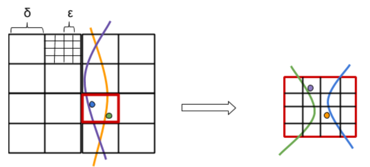
Following the general approach in [2], we use a suitable duality, with some care. We write , for suitable parameters , and , whose concrete values are fixed later, and apply the decomposition scheme developed in [2] tailored to the case at hand. Specifically, we consider the coarser grid in the primal space, of cell dimensions , where is is the constant from Lemma 2.2, that tiles up the domain of possible camera positions. For each cell of , let denote the set of surfaces that cross either or one of the eight cells adjacent to in the -directions.222The choice of , is arbitrary, but it is natural for the analysis, given in the appendix. The duality is illustrated in Figure 2.
We discretize the set of all possible positions of the camera by the vertices of the finer grid , defined as , with replacing , that tiles up . The number of these candidate positions is . For each vertex , we want to approximate the number of surfaces that are -incident to , and output the vertex with the largest count as the best candidate for the position of the camera. Let be the subset of contained in . We ensure that the boxes of are pairwise disjoint by making them half open, in the sense that if is the vertex of a box that has the smallest coordinates, then the box is defined by , , , . This makes the sets pairwise disjoint as well. Put and . We have for each . Since the surfaces are two-dimensional algebraic surfaces of constant degree, each of them crosses cells of , so we have .
We now pass to the dual five-dimensional space. Each point in that space represents a correspondence . We use the first three components as the first three coordinates, but modify the - and -coordinates in a manner that depends on the primal cell . Let be the midpoint of the primal box . For each we map , where , to the point , where and , with and as given in (3). We have
Corollary 3.1.
If crosses then , for some absolute constant , provided that the following two properties hold, for some absolute constant (the constant depends on ).
(i) , and
(ii) , where are the -coordinates of the center of .
Proof 3.2.
We take the provided by Corollary 3.1 as the in the definition of and . We map each point to the dual surface . Using (3), we have
By Corollary 3.1, the points , for the surfaces that cross , lie in the region . We partition into a grid of small congruent boxes, each of dimensions .
Exactly as in the primal setup, we make each of these boxes half-open, thereby making the sets of dual vertices in the smaller boxes pairwise disjoint. We assign to each of these dual cells the set of dual points that lie in , and the set of the dual surfaces that cross either or one of the eight cells adjacent to in the -directions. Put and . Since the dual cells are pairwise disjoint, we have . Since the dual surfaces are three-dimensional algebraic surfaces of constant degree, each of them crosses grid cells, so .
We compute, for each dual surface , the sum , over the dual cells that are either crossed by or that one of their adjacent cells in the -directions is crossed by . We output the vertex of with the largest resulting count, over all primal cells .
The following theorem establishes the correctness of our technique. Its proof is given in Appendix B.
Theorem 3.3.
Suppose that for every cell and for every point and every such that intersects either or one of its adjacent cells in the -directions, we have that, for some absolute constant ,
(i) ,
(ii) , and
(iii) .
Then (a) For each , every pair at frame distance is counted (as an -incidence of ) by the algorithm. (b) For each , every pair that we count lies at frame distance , for some constant depending on .
3.1. Running time analysis
The cost of the algorithm is clearly proportional to over all primal cells and the dual cells associated with each cell . We have
Optimizing the choice of and , we choose and . These choices make sense as long as each of , lies between and . That is, and , or , where and are absolute constants (that depend on ).
If , we use only the primal setup, taking (for the primal subdivision). The cost is then Similarly, if , we use only the dual setup, taking and , and the cost is thus Adding everything together, to cover all three subranges, the running time is then Substituting , we get a running time of The first term dominates when and . In conclusion, we have the following result.
Theorem 3.4.
Given data points that are seen (and identified) in a two-dimensional image taken by a vertically positioned camera, and an error parameter , where the viewed points satisfy the assumptions made in Theorem 3.3, we can compute, in time, a vertex of that maximizes the approximate count of -incident correspondences, where “approximate” means that every correspondence whose surface is at frame distance at most from is counted and every correspondence that we count lies at frame distance at most from , for some fixed constant .
Restricting ourselves only to grid vertices does not really miss any solution. We only lose a bit in the quality of approximation, replacing by a slightly large constant multiple thereof, when we move from the best solution to a vertex of its grid cell.
4. Geometric proximity via canonical surfaces
In this section we present a general technique to preprocess a set of algebraic surfaces into a data structure that can answer approximate incidences queries. In this technique we round the original surfaces into a set of canonical surfaces, whose size depends only on , such that each original surface has a canonical surface that is “close” to it. Then we build an octree-based data structure for approximate incidences queries with respect to the canonical surfaces. However, to reduce the number of intersections between the cells of the octree and the surfaces, we further reduce the number of surfaces as we go from one level of the octree to the next, by rounding them in a coarser manner into a smaller set of surfaces.
This technique has been introduced by Fonseca and Mount [3] for the case of hyperplanes. We describe as a warmup step, in Section C of the appendix, our interpretation of their technique applied to hyperplanes. We then extend here the technique to general surfaces, and apply it to the specific instance of 2-surfaces in 4-space that arise in the camera pose problem.
We have a set of -dimensional surfaces in that cross the unit cube , and a given error parameter . We assume that each surface is given in parametric form, where the first coordinates are the parameters, so its equations are
Moreover, we assume that each is defined in terms of essential parameters , and additional free additive parameters , one free parameter for each dependent coordinate. Concretely, we assume that the equations defining the surface , parameterized by and (we then denote as ), are
For each equation of the surface that does not have a free parameter in the original expression, we introduce an artificial free parameter, and initialize its value to . (We need this separation into essential and free parameters for technical reasons that will become clear later.) We assume that (resp., ) varies over (resp., ).
Remark. The distinction between free and essential parameters seems to be artificial, but yet free parameters do arise in certain basic cases, such as the case of hyperplanes discussed in Section C of the appendix. In the case of our 2-surfaces in 4-space, the parameter is free, and we introduce a second artificial free parameter into the equation for . The number of essential parameters is (they are ,,, and ).
We assume that the functions are all continuous and differentiable, in all of their dependent variables , and (this is a trivial assumption for ), and that they satisfy the following two conditions.
(i) Bounded gradients. for each , for any and any , where is some absolute constant. Here (resp., ) means the gradient with respect to only the variables (resp., ).
(ii) Lipschitz gradients. for each , for any and any , , where is some absolute constant. This assumption is implied by the assumption that all the eigenvalues of the mixed part of the Hessian matrix have absolute value bounded by .
4.1. Canonizing the input surfaces
We first replace each surface by a canonical “nearby” surface . Let where is the constant from Condition (ii). We get from (resp., from ) by rounding each coordinate in the essential parametric domain (resp., in the parametric domain ) to a multiple of . Note that each of the artificial free parameters (those that did not exist in the original equations) has the initial value for all surfaces, and remains in the rounded surfaces. We get canonical rounded surfaces, where is the number of original parameters, that is, the number of essential parameters plus the number of non-artificial free parameters; in the worst case we have .
For a surface and its rounded version we have, for each ,
where is some intermediate value, which is irrelevant due to Condition (i).
We will use the -norm of the difference vector as the measure of proximity between the surfaces and at , and denote it as . The maximum measures the global proximity of the two surfaces. (Note that it is an upper bound on the Hausdorff distance between the two surfaces.) We thus have when is the canonical surface approximating .
We define the weight of each canonical surface to be the number of original surfaces that got rounded to it, and we refer to the set of all canonical surfaces by .
4.2. Approximately counting -incidences
We describe an algorithm for approximating the -incidences counts of the surfaces in and the vertices of a grid of side length .
We construct an octree decomposition of , all the way to subcubes of side length such that each vertex of is the center of a leaf-cube. We propagate the surfaces of down this octree, further rounding each of them within each subcube that it crosses.
The root of the octree corresponds to , and we set . At level of the recursion, we have subcubes of of side length . For each such , we set to be the subset of the surfaces in (that have been produced at the parent cube of ) that intersect . We now show how to further round the surfaces of , so as to get a coarser set of surfaces that we associate with , and that we process recursively within .
At any node at level of our rounding process, each surface of is of the form , for where , and .
(a) For each the function is a translation of . That is for some constant . Thus the gradients of also satisfy Conditions (i) and (ii).
(b) is some vector of essential parameters, and each coordinate of is an integer multiple of , where .
(c) is a vector of free parameters, each is a multiple of .
Note that the surfaces in , namely the set of initial canonical surfaces constructed in Section 4.1, are of this form (for and ). We get from by the following steps. The first step just changes the presentation of and , and the following steps do the actual rounding to obtain .
-
(1)
Let be the point in of smallest coordinates and set . We rewrite the equations of each surface of as follows: , for , where , and , for . Note that in this reformulation we have not changed the essential parameters, but we did change the free parameters from to , where depends on , , , and . Note also that for .
-
(2)
We replace the essential parameters of a surface by , which we obtain by rounding each coordinate of to the nearest integer multiple of . So the rounded surface has the equations , for . Note that we also have that , for .
-
(3)
For each surface, we round each free parameter , , to an integral multiple of , and denote the rounded vector by . Our final equations for each rounded surface that we put in are for .
By construction, when and and and get rounded to the same vectors and then the corresponding two surfaces in get rounded to the same surface in . The weight of each surface in is the sum of the weights of the surfaces in that got rounded to it, which, by induction, is the number of original surfaces that are recursively rounded to it. In the next step of the recursion the ’s of the parametrization of the surfaces in are the functions defined above.
The total weight of the surface in for a leaf cell is the approximate -incidences count that we associate with the center of .
4.3. Error analysis
We now bound the error incurred by our discretization. We start with the following lemma, whose proof is given in Appendix .
Lemma 4.1.
Let be a cell of the octtree and let , for be a surface obtained in Step 1 of the rounding process described above. For any , for any , and for each , we have
| (5) |
where is the constant of Condition (ii), and consists of the first coordinates of the point in of smallest coordinates.
Lemma 4.2.
For any , for any , , and for each , we have
| (6) |
where is the constant of Condition (ii).
Proof 4.3.
We now bound the number of surfaces in . Since and each of its coordinates is a multiple of , we have at most different values for . To bound the number of possible values of , we prove the following lemma (see the appendix for the proof).
Lemma 4.4.
Let , for , be a surface in . For each , we have , where is the constant of Condition (i).
Lemma 4.4 implies that each , , has only possible values, for a total of at most possible values for . Combining the number of possible values for and , we get that the number of newly discretized surfaces in is
| (7) |
It follows that each level of the recursive octree decomposition generates
re-discretized surfaces, where the first factor in the left-hand side expression is the number of cubes generated at this recursive level, and the second factor is the one in (7).
Summing over the recursive levels , where the cube size is at level , we get a total size of . We get different estimates for the sum according to the sign of . If the sum is . If the sum is . If the sum is Accordingly, the overall size of the structure, taking also into account the cost of the first phase, is
| (8) |
The following theorem summarizes the result of this section. Its proof follows in a straightforward way from the preceding discussion from Lemma 4.2, analogously to the proof of Lemma 4.4 in the appendix.
Theorem 4.5.
Let be a set of surfaces in that cross the unit cube , given parametrically as for , where the functions satisfy conditions (i) and (ii), and . Let be the -grid within . The algorithm described above reports for each vertex of an approximate -incidences count that includes all surfaces at distance at most from and may include some surfaces at distance at most from . The running time of this algorithm is proportional to the total number of rounded surfaces that it generates, which is given by Equation (8), plus an additive term for the initial canonization of the surfaces.
We can modify our data structure so that it can answer approximate or exact -incidence queries as we describe in Section C of the appendix for the case of hyperplanes.
5. Experimental Results
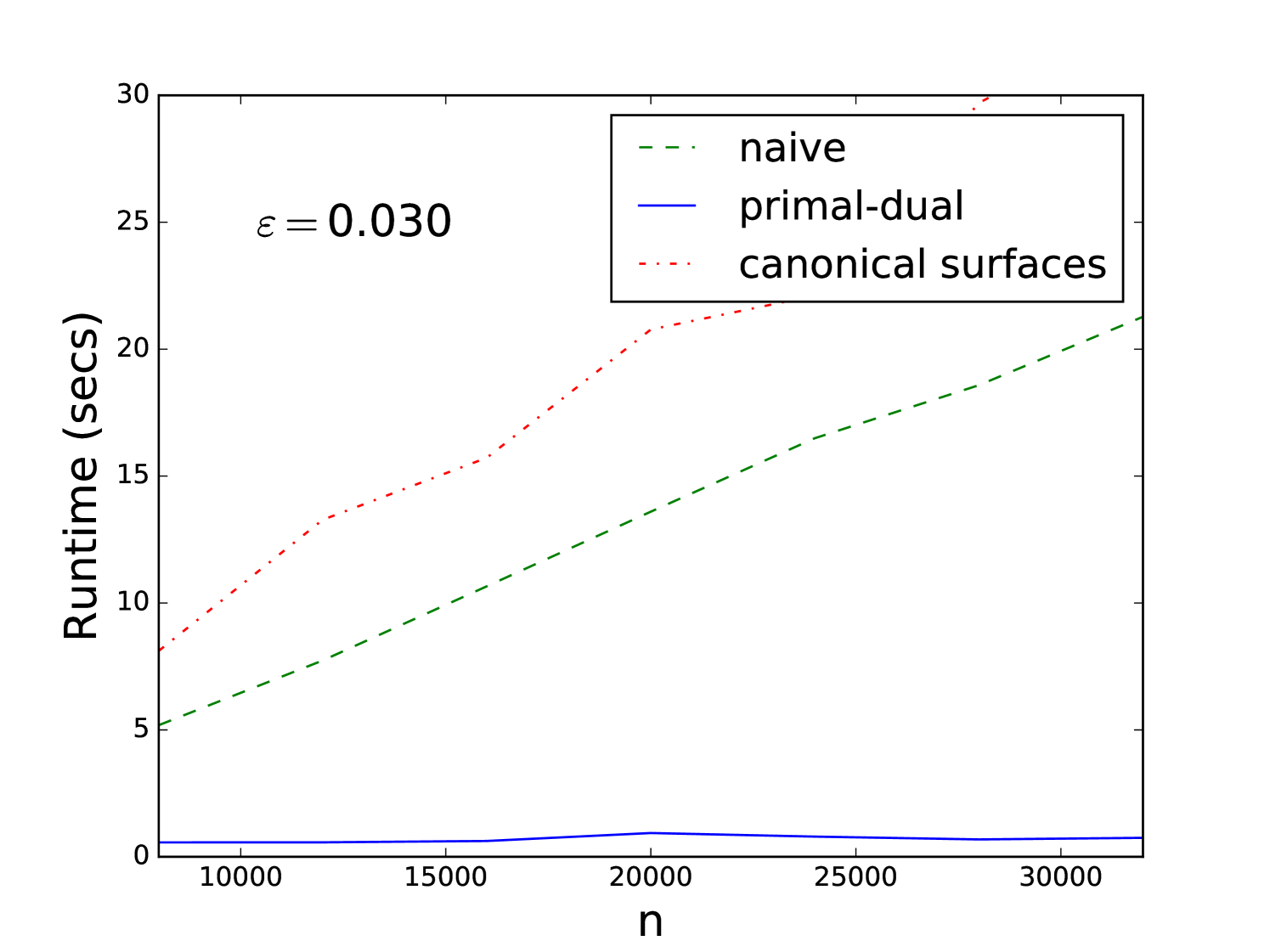
The goal of the experimental results is to show the practical relation between the naive, the primal-dual and the general canonical surfaces algorithms. It is not our intention to obtain the fastest possible code, but to obtain a platform for fair comparison between the techniques. We have performed a preliminary experimental comparison using synthetic as well as real-world data. We focus on values of that are practical in real applications. Typically, we have - D points bounded by a rectangle of size 100-150 meters and the uncertainty is around 3m (so the relative error is ). The three methods that we evaluate are:
In all experiments we normalize the data, so that the camera position () and the D points lie in the unit box , and the forth parameter () representing the camera orientation lies in .
5.1. Random synthetic data
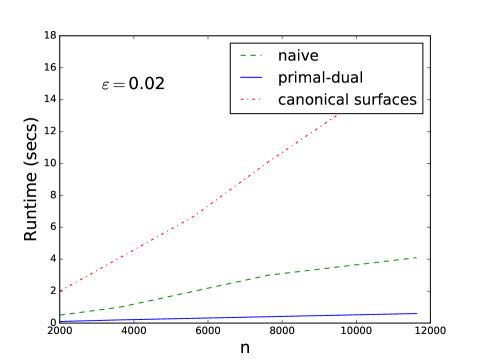
Starting from a fixed known camera pose, we generate a set of uniformly sampled D points which are projected onto the camera image plane using Eq. (1). To model outliers in the association process we use random projections for 90% of the points, resulting in an inlier ratio of . We add Gaussian noise of zero mean and to the coordinates of each point. This provides us with D-D correspondences that are used for estimating the camera pose. We apply the three algorithms above and measure the run-times, where each algorithm is tested for its ability to reach approximately the (known) solution. We remark that the actual implementation may be slowed down by the (constant) cost of some of its primitive operations, but it can also gain efficiency from certain practical heuristic improvements. For example, in contrast to the worst case analysis, we could stop the recursion in the algorithm of Section 4, at any step of the octree expansion, whenever the maximum incidence count obtained so far is larger than the number of surfaces crossing a cell of the octree. The same applies for the primal-dual technique in the dual stage. On the other hand, finding whether or not a surface crosses a box in pose space, takes at least the time to test for intersections of the surface with 32 edges of the box, and this constant affects greatly the run-time. The bound in the canonical surfaces algorithm is huge and has no effect in practice for this problem. For this reason, the overall number of surfaces that we have to consider in the recursion can be very large. The canonical surfaces algorithm in our setting does not change much with because we are far from the second term effect. We show in Figure 3, a comparison of the three algorithms.
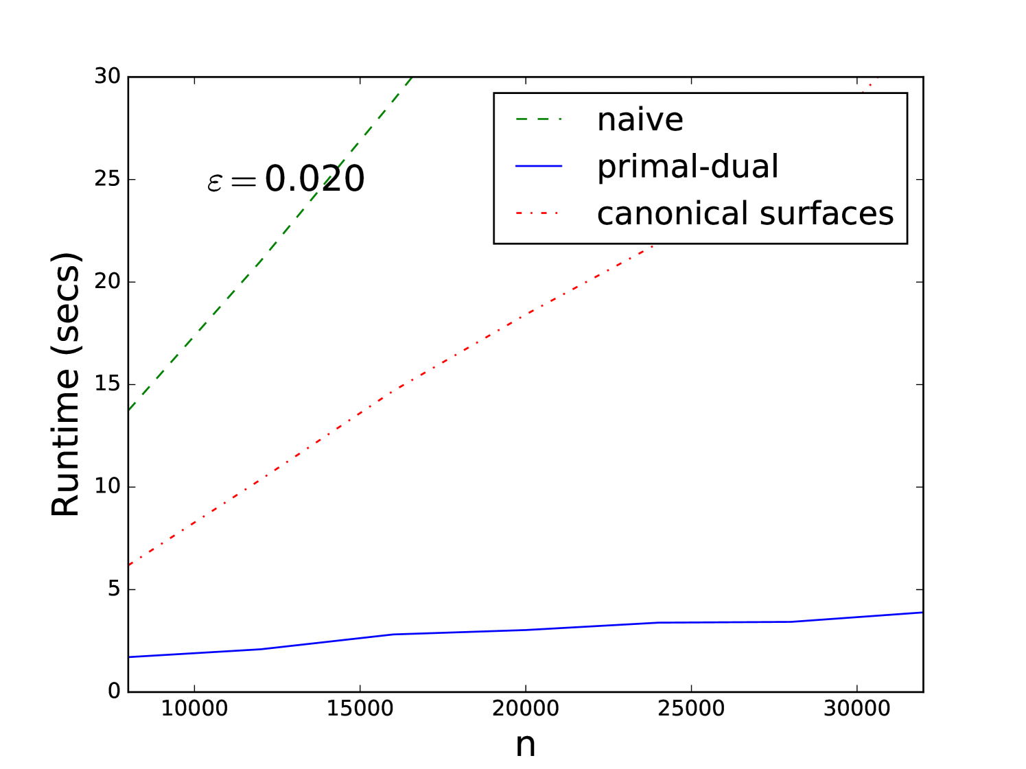
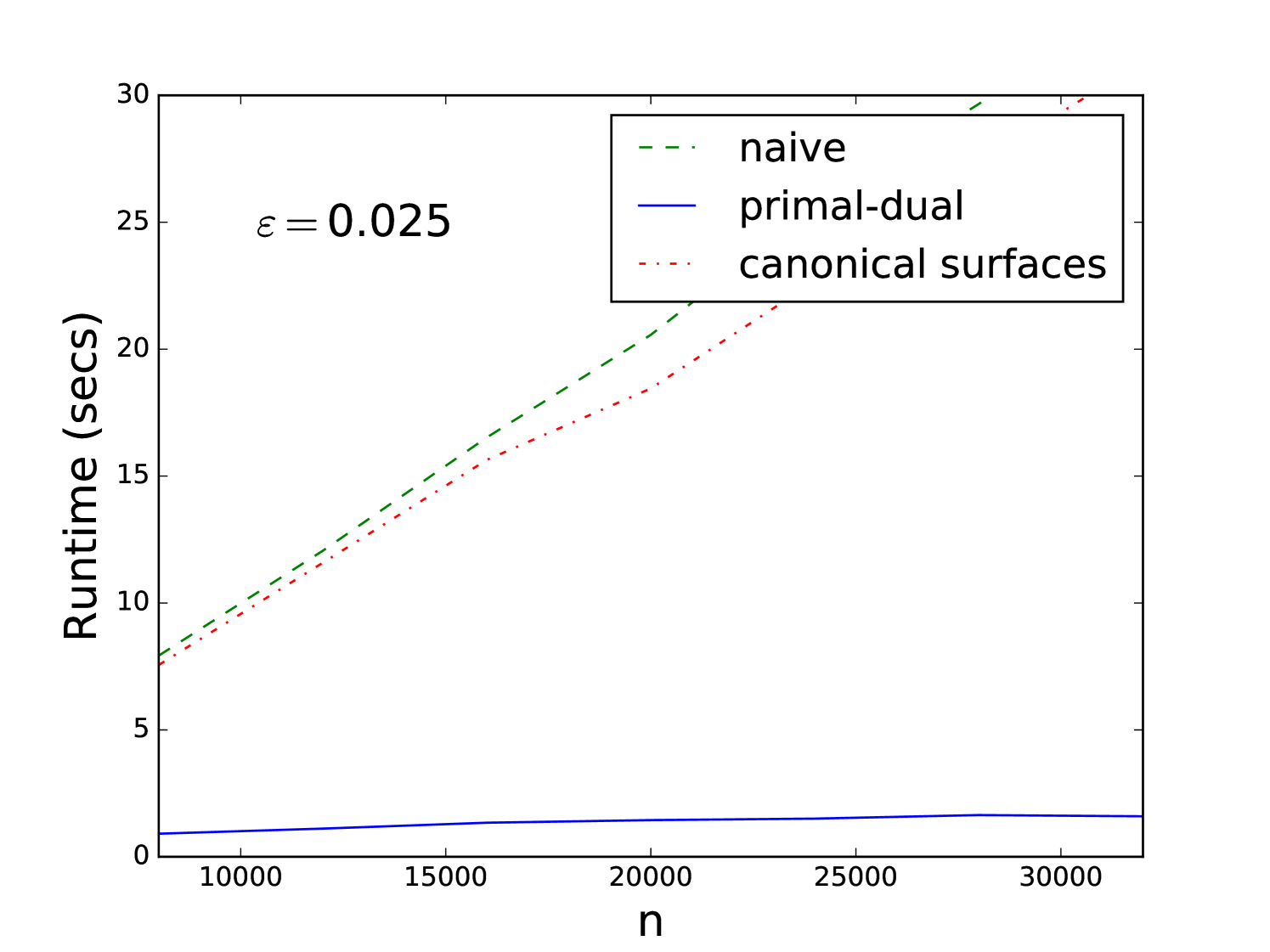
The computed camera poses corresponding to Figure 3, obtained by the three algorithm for various problem sizes, are displayed in Table 1, compared to the known pose. The goal here is not to obtain the most accurate algorithm but to show that they are comparable in accuracy in this setting so the runtime comparison is fair.
| n | x(N/PD/C) | y(N/PD/C) | z(N/PD/C) | (N/PD/C) |
|---|---|---|---|---|
| 8000 | 0.31/0.31/0.28 | 0.22/0.2/0.18 | 0.1/0.12/0.09 | 0.55/0.66/0.59 |
| 12000 | 0.31/0.33/0.28 | 0.22/0.17/0.19 | 0.1/0.1/0.1 | 0.55/0.65/0.6 |
| 24000 | 0.31/0.3/0.28 | 0.22/0.2/0.18 | 0.1/0.1/0.09 | 0.55/0.61/0.59 |
| 32000 | 0.31/0.27/0.28 | 0.22/0.2/0.19 | 0.1/0.08/0.09 | 0.55/0.57/0.59 |
| True pose | 0.3 | 0.2 | 0.1 | 0.6 |
5.2. Real-world data
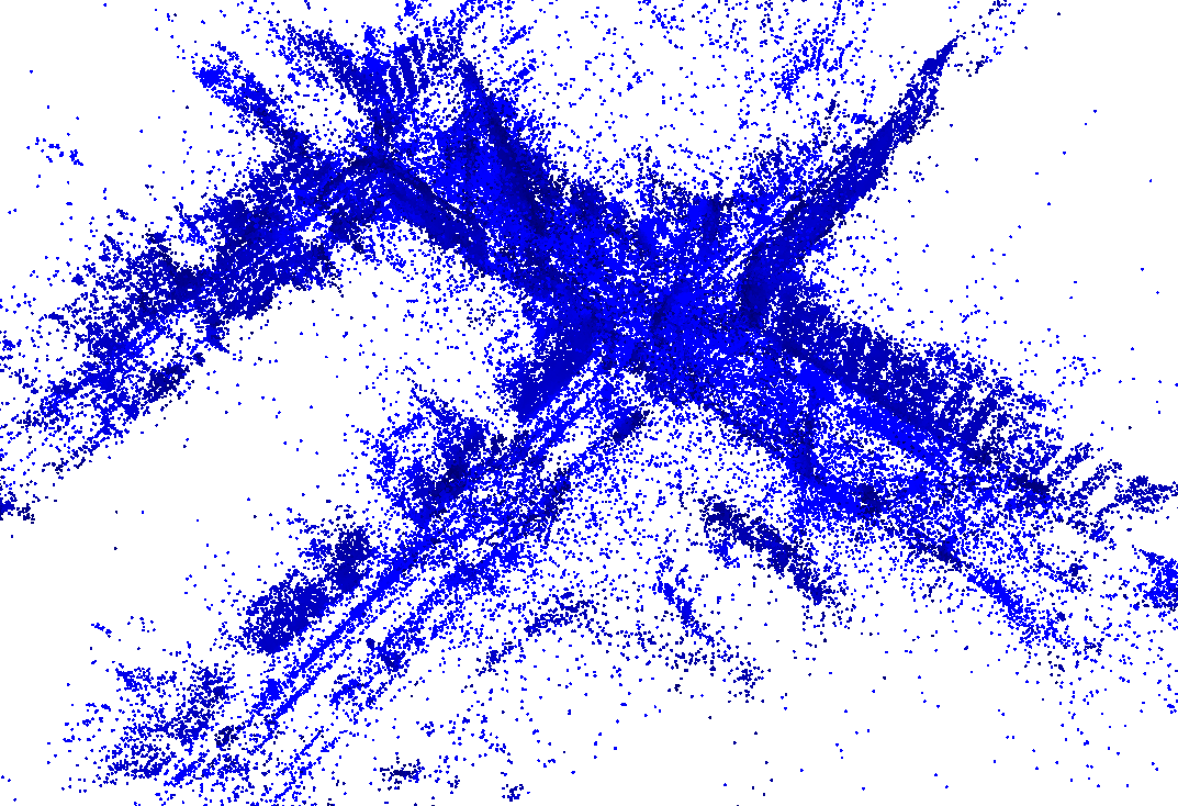
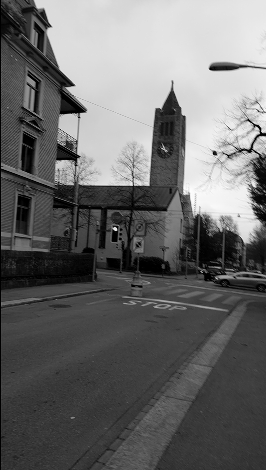
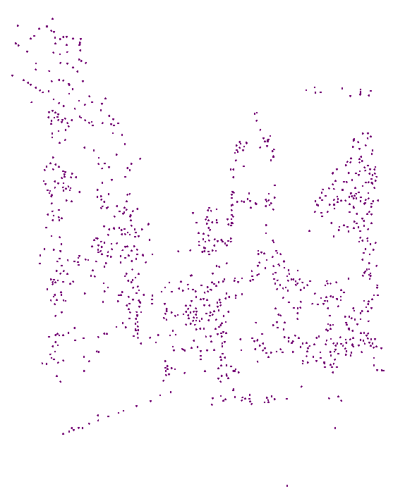
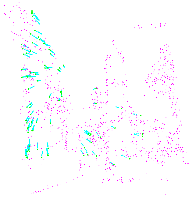
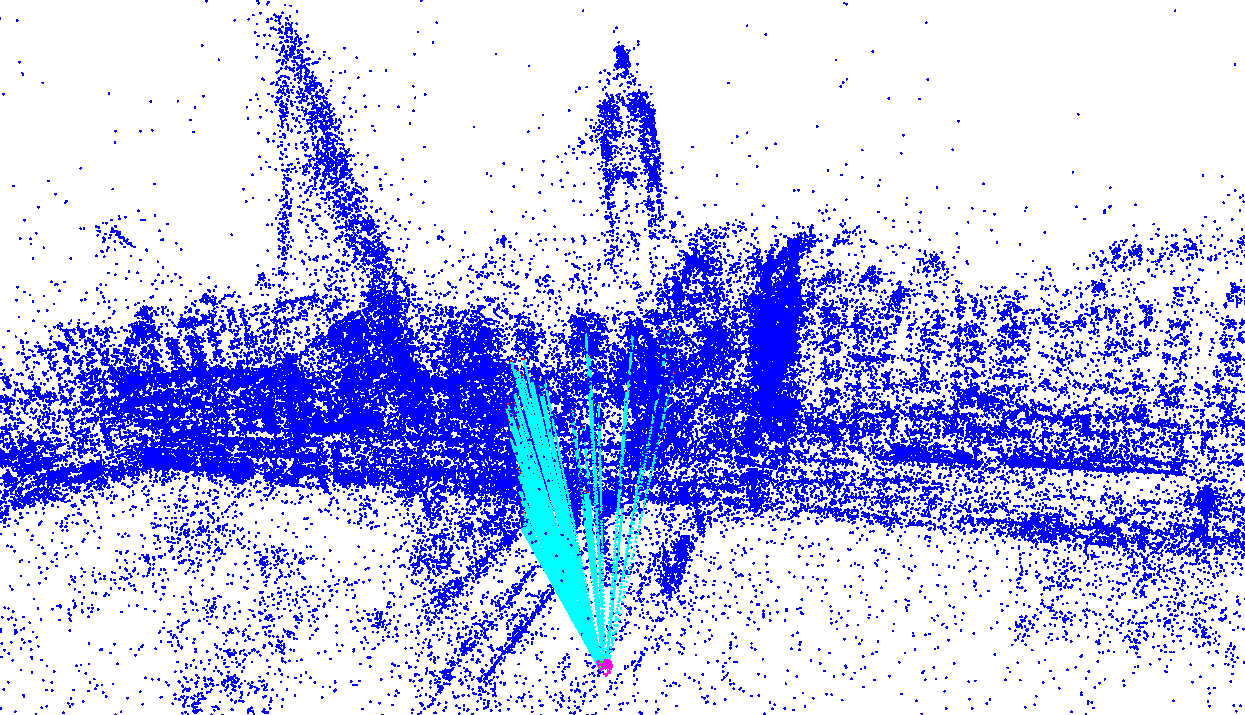
We evaluated the performance of the algorithms also on real-world datasets for which the true camera pose is known. The input is a set of correspondences, each represented by a -tuple , where are the coordinates of a salient feature in the scene and is its corresponding projection in the camera frame. We computed the camera pose from these matches using both primal-dual and naive algorithms and compared the poses to the true one. An example of the data we have used is shown in Figure 4.
We evaluated the runtime for different problem sizes and checked the correctness of the camera pose approximation when the size increased. To get different input sizes, we added random correspondences to a base set of actual correspondences. The number of random correspondences determines the input size but also the fraction of good correspondences (percentage of inliers) which goes down with increased input size (the number of inliers in real world cases is typically 10%). We show the same plots as before in Figure 5 and Table 2.
| n | x | y | z | |
|---|---|---|---|---|
| 2000 | 0.26 | 0.62 | 0.06 | 0.72 |
| 3626 | 0.36 | 0.56 | 0.12 | 0.52 |
| 5626 | 0.38 | 0.60 | 0.12 | 0.62 |
| 7626 | 0.40 | 0.64 | 0.08 | 0.57 |
| 11626 | 0.43 | 0.68 | 0.13 | 0.63 |
| True pose | 0.37 | 0.59 | 0.06 | - |
6. Future work
We note that similar approaches can be applied for computing the relative pose [10] between two cameras (that look at the same scene), except that the pose estimation then uses D-D matches between the two images (rather than 2D-3D image-to-model correspondences). Determining the relative motion between images is a prerequisite for stereo depth estimation [12], in multi-view geometry [7], and for the initialization of the view graph [15, 16] in SfM, and is therefore an equally important task in computer vision. In addition, in future work we want to also consider the case of a generalized or distributed camera setup and likewise transform the camera posing problem to an -incidence problem.
References
- [1] S. Agarwal, N. Snavely, I. Simon, S. M. Seitz, and R. Szeliski. Building rome in a day. In Commun. ACM 54(10), pages 105–112. ACM, 2011.
- [2] D. Aiger, H. Kaplan, and M. Sharir. Output sensitive algorithms for approximate incidences and their applications. In Computational Geometry, to appear. Also in European Symposium on Algorithms, volume 5, pages 1–13, 2017.
- [3] G. D. Da Fonseca and D. M. Mount. Approximate range searching: The absolute model. Computational Geometry, 43(4):434–444, 2010.
- [4] M. A. Fischler and R. C. Bolles. Random sample consensus: A paradigm for model fitting with applications to image analysis and automated cartography. Communications of the ACM, 24(6):381–395, 1981.
- [5] C. Häne, L. Heng, G. H. Lee, F. Fraundorfer, P. Furgale, T. Sattler, and M. Pollefeys. 3d visual perception for self-driving cars using a multi-camera system: Calibration, mapping, localization, and obstacle detection. Image and Vision Computing, 68:14–27, 2017.
- [6] B. M. Haralick, C.-N. Lee, K. Ottenberg, and M. Nölle. Review and analysis of solutions of the three point perspective pose estimation problem. International Journal of Computer Vision, 13(3):331–356, 1994.
- [7] R. Hartley and A. Zisserman. Multiple View Geometry in Computer Vision. Cambridge university press, 2003.
- [8] G. Klein and D. Murray. Parallel tracking and mapping for small ar workspaces. In ISMAR, pages 83–86. IEEE, 2009.
- [9] S. Middelberg, T. Sattler, O. Untzelmann, and L. Kobbelt. Scalable 6-dof localization on mobile devices. In European Conference on Computer Vision, pages 268–283. Springer, 2014.
- [10] D. Nistér. An efficient solution to the five-point relative pose problem. IEEE Transactions on Pattern Analysis and Machine Intelligence, 26(6):756–770, 2004.
- [11] M. Pollefeys, L. Van Gool, M. Vergauwen, F. Verbiest, K. Cornelis, J. Tops, and R. Koch. Visual modeling with a hand-held camera. International Journal of Computer Vision, 59(3):207–232, 2004.
- [12] D. Scharstein and R. Szeliski. A taxonomy and evaluation of dense two-frame stereo correspondence algorithms. International Journal of Computer Vision, 47(1-3):7–42, 2002.
- [13] J. L. Schonberger and J.-M. Frahm. Structure-from-motion revisited. In Proceedings of the IEEE Conference on Computer Vision and Pattern Recognition, pages 4104–4113, 2016.
- [14] C. Sweeney, J. Flynn, B. Nuernberger, M. Turk, and T. Höllerer. Efficient computation of absolute pose for gravity-aware augmented reality. In ISMAR, pages 19–24. IEEE, 2015.
- [15] C. Sweeney, T. Sattler, T. Hollerer, M. Turk, and M. Pollefeys. Optimizing the viewing graph for structure-from-motion. In Proceedings of the IEEE International Conference on Computer Vision, pages 801–809, 2015.
- [16] C. Zach, M. Klopschitz, and M. Pollefeys. Disambiguating visual relations using loop. constraints. In Computer Vision and Pattern Recognition, pages 1426–1433. IEEE, 2010.
- [17] B. Zeisl, T. Sattler, and M. Pollefeys. Camera pose voting for large-scale image-based localization. In Proceedings of the IEEE International Conference on Computer Vision, pages 2704–2712, 2015.
Appendix A Omitted proofs
In all experiments we normalize the data, so that the camera position () and the D points lie in the unit box , and the forth parameter () representing the camera orientation lies in . Let , We apply the three algorithms above and measure the run-times, where each algorithm is tested for its ability to reach approximately the (known) solution. We remark that the actual implementation may be slowed down by the (constant) cost of some of its primitive operations, but it can also gain efficiency from certain practical heuristic improvements. For example, in contrast to the worst case analysis, we could stop the recursion in the algorithm of Section 4, at any step of the octree expansion, whenever the maximum incidence count obtained so far is larger than the number of surfaces crossing a cell of the octree. The same applies for the primal-dual technique in the dual stage. On the other hand, finding whether or not a surface crosses a box in pose space, takes at least the time to test for intersections of the surface with 32 edges of the box, and this constant affects greatly the run-time. The bound in the canonical surfaces algorithm is huge and has no effect in practice for this problem. For this reason, the overall number of surfaces that we have to consider in the recursion can be very large. The canonical surfaces algorithm in our setting does not change much with because we are far from the second term effect. We show in Figure 3, a comparison of the three algorithms. Since we have that , . We want to show that for some constant that depends on .
Regarding and as functions of , we compute their gradients as follows.
and
Conditions (i) and (ii) in the lemma, plus the facts that we restrict both and to lie in the bounded domain , and that is also at most , are then easily seen to imply that the -gradients are at most , for some constant that depends on , and so and , and the lemma follows.
Proof A.1 (Proof of Lemma 2.2:).
Let
| (9) | ||||
Since we have that .
Since the Equations (2) are the inverse system of those of (1), we can rewrite (9) as
Hence
It follows right away that (recall that all the points lie in the unit cube). For the other difference, writing
(with the other parameters being fixed), we get
As is easily verified, we have
Since , and , the denominator of is bounded away from zero (assuming that is sufficiently small), and for , where is some fixed positive constant. This implies that , and the lemma follows.
Proof A.2 (Proof of Theorem 3.3. Part (a):).
Let be a pair at frame distance . By Lemma 2.2 and the definition of , there exists a cell such that and .
By definition, the surface contains the point
where and are given by (9). Since , the points and lie at -distance at most , therefore where is the cell that contains .
Together, these two properties imply that is counted by the algorithm. Moreover, since we kept both primal and dual boxes pairwise disjoint, each such pair is counted exactly once.
Part (b): Let be an -incident pair that we encounter, where and are encoded as above. That is, crosses the primal cell of that contains , or a neighboring cell in the -directions, and crosses the dual cell that contains , or a neighboring cell in the -directions. This means that (or a neighboring cell) contains a point , and (or a neighboring cell) contains a point . The former containment means that
and that
To interpret the latter containment, we write, using the definition of , , and the fact that ,
where , and where is the centerpoint of , and
where
By definition (of , , and the frame distance), we have
which we can bound by writing
We are given that
so it remains to bound the other term in each of the two right-hand sides. Consider for example the expression
| (10) |
Write and , for suitable vectors . We expand the expression up to second order, by writing
where (resp., ) denotes the gradient with respect to the variables (resp., ), and where (resp., , ) denotes the Hessian submatrix of second derivatives in which both derivatives are with respect to (resp., both are with respect to , one derivative is with respect to and the other is with respect to ).
Substituting in (10), we get that, up to second order,
where is the maximum of the absolute values of all the “mixed” second derivatives. (Note that the mixed part of the Hessian of the Hessian arises also in the analysis of the algorithm in Section 4.) Arguing as in the preceding analysis and using the assumptions in the theorem, one can show that all these derivatives are bounded by some absolute constants, concluding that
which implies that
Applying an analogous analysis to , we also have
Together, these bounds complete the proof of part (b) of the theorem.
Proof A.3 (Proof of Lemma 4.1:).
Fix , consider the function
and recall our assumption that . Then we can also write the left-hand side of (5) as . By the intermediate value theorem, it can be written as
for some intermediate value (that depends on and ). By definition, we have,
| (11) |
whose norm is bounded by by Condition (ii). Using the Cauchy-Schwarz inequality, we can thus conclude that
as asserted.
Proof A.4 (Proof of Lemma 4.4:).
Each surface in meets . That is, there exists a point in that lies on , so we have for each , where . Hence, for some intermediate value , we have
where the first inequality follows by the triangle inequality, the second follows since , the third by the intermediate value theorem and the Cauchy-Schwarz inequality, and the fourth by Condition (i).
Appendix B A simple algorithm
We present a simple naive solution which does not require any of the sophisticated machinery developed in this work. It actually turns out to be the most efficient solution when is small.
We construct a grid over , of cells , each of dimensions , where is the constant of Lemma 2.2. (We use this non-square grid since we want to find -approximate incidences in terms of frame distance.) For each cell of we compute the number of surfaces that intersect .
Consider now a shifted version of in which the vertices of are the centers of the cells of . To report how many surfaces are within frame distance from a vertex , we return the count of the cell of whose center is . By Lemma 2.2 and Lemma 2.1, this includes all surfaces at frame distance from , but may also count surfaces at frame distance at most from , where is the constant in Lemma 2.1. (The distance from to the farthest corner of its cell is .)
It takes time to construct this data structure. Indeed, cell boundaries reside on hyperplanes, so we compute the intersection curve of each surface with each of these hyperplanes, in a total of time. Then, for each such curve we find the cell boundaries that it intersects within its three-dimensional hyperplane in time. We summarize this result in the following theorem.
Theorem B.1.
The algorithm described above approximates the the number of surfaces that are at distance to each vertex where is an grid in . (The approximation is in the sense defined above.)
Proof B.2.
In fact we can find for each vertex of , the exact number of -incident surfaces (i.e. surfaces at distance at most from ). For this we keep with each cell of , the list of the surfaces that intersect . Then for each vertex we traverse the surfaces stored in its cell and check which of them is within frame distance from . The asymptotic running time is still .
If we want to get an incidences counts of vertices of a finer grid that , we use a union of several shifted grids as above. This also allows to construct a data structure that can return an -incidences count of any query point.
For the camera pose problem we use the vertex of of largest -incidences count as the position of the camera.
Appendix C Geometric proximity via canonical surfaces: The case of hyperplanes
We have a set of hyperplanes in that cross the unit cube , and a given error parameter . Each hyperplane is given by an equation of the form . We assume, for simplicity, that for each and for each . Moreover, since crosses , we have , as is easily checked. (This can always be enforced by rewriting the equation turning the with the coefficient of largest absolute value into the independent coordinate.)
For our rounding scheme we define . We discretize each hyperplane as follows. Let the equation of be . We replace each by the integer multiple of that is nearest to it, and do the same for . Denoting these ‘snapped’ values as and , respectively, we replace by the hyperplane , given by . For any , the -vertical distance between and at is
We define the weight of each canonical hyperplane to be the number of original hyperplanes that got rounded to it, and we refer to the set of all canonical hyperplanes by .
We describe a recursive procedure that approximates the number of -incident hyperplanes of to each vertex of a -grid that tiles up . Specifically, for each vertex of we report a count that includes all hyperplanes in that are at Euclidean distance at most from but it may also count hyperplanes of that are at distance up to from .
Our procedure constructs an octree decomposition of , all the way to subcubes of side length . (We assume that is a negative power of to avoid rounding issues.) We shift the grid such that its vertices are centers of these leaf-subcubes. At level of the recursive construction, we have subcubes of side length . For each such we construct a set of more coarsely rounded hyperplanes. The weight of each hyperplane in is the sum of the weights of the hyperplanes in the parent cube of that got rounded to , which, by induction, is the number of original hyperplanes that are rounded to it (by repeated rounding along the path in the recursion tree leading to ).
At the root, where , we set (where each has the initial weight of the number of original hyperplanes rounded to it, as described above). At any other cell we obtain by applying a rounding step to the set of the hyperplanes of that intersect .
The coarser discretization of the hyperplanes of that produces the set proceeds as follows. Let denote the coordinates of the corner of with smallest coordinates, so .
Let be a hyperplane of , and rewrite its equation as
This rewriting only changes the value of but does not affect the ’s. Since crosses , we have (and for each ). We now re-discretize each coefficient (resp., ) to the integer multiple of (resp., ) that is nearest to it. Denoting these snapped values as and , respectively, we replace by the hyperplane given by
This re-discretization of the coefficients is a coarsening of the discretization of the hyperplanes in . The set contains all the new, more coarsely rounded hyperplanes that we obtain from the hyperplanes in in this manner. Note that several hyperplanes in may be rounded to the same hyperplane in . We set the weight of each hyperplane in to be the sum of the weights of the hyperplanes in that got rounded to it. (Note that although every hyperplane of crosses , such an may get rounded to a hyperplane that misses , in which case it is not represented by any hyperplane in .)
For any , the -vertical distance between and at is
Since the original value of is in and we round it to an integer multiple of , the hyperplanes in have possible values for each coefficient . Furthermore, these hyperplanes also have possible values for , because for every hyperplane in (since it intersects ). It follows that , and the total size of all sets , over all cells at the same level of the octree, is .
Finally, at every leaf of the octree we report the sum of the weights of the hyperplanes in as the approximate -incidences count of the vertex of at the center of .
Theorem C.1.
Let be a set of hyperplanes in that cross the unit cube , and let be the -grid within . The algorithm described above reports for each vertex of an approximate -incidences count that includes all hyperplanes at Euclidean distance at most from and may include some hyperplanes at distance at most from . The running time of this algorithm is .
Proof C.2.
Let , and consider a hyperplane at distance at most from . The hyperplane is rounded to a hyperplane which is at distance at most from ,333The distance between two hyperplanes is defined to be the maximum vertical distance between them. and thereby at distance at most from . The hyperplane is further rounded to other hyperplanes while propagating down the octree. The distance from from the hyperplane that it is rounded to in is at most , and, in general the distance of from any hyperplane , that it is rounded to at any level , is at most . (Note that is rounded to different hyperplanes in different cells of level .) Therefore the distance of from is at most (since ). It follows that is rounded to some hyperplane that crosses the cell that contains , at each level of the octree. In particular is (repeatedly) rounded to some hyperplane at the leaf containing and is included in the weight of some hyperplane at that leaf.
Consider now a hyperplane that is rounded to some hyperplane at the leaf containing . The hyperplane is at distance at most from . Therefore is at distance at most from the boundary of the leaf-cell containing . The distance of to the boundary of the leaf-cell containing it is at most , so the distance of from is at most .
The running time follows from the fact that the total size of the sets for all cells at a particular level of the quadtree is and there are levels.
Note that if we consider an arbitrary point then each hyperplane at distance at most from is included in the approximate count of at least one of the vertices of the grid surrounding . In this rather weak sense, the largest approximate incidences count of a vertex of can be considered as an approximation to the number of -close hyperplanes to the point with the largest number of -close hyperplanes.
Our octree data structure can give an approximate -incidences count for any query point (albeit with somewhat worse constants). For this we construct a constant number of octree structures over shifted (by intergral multiple of ) grids of a somewhat larger side-length, say . The grids are shifted such that each cell of a finer grid of side length is centered in a larger grid cell of one of our grids, say . We use to answer queries that lie in , by returning the sum of the weights of the hyperplanes in where is the leaf of containing .
We can also modify this data structure such that it can answer -incidences queries exactly. That is, given a query point , it can count (or report) the number of hyperplanes at distance at most from and only these hyperplanes. To do this we maintain pointers from each hyperplane in to the hyperplanes in that got rounded to . To answer a query , we find the leaf cell containing and then we traverse back the pointers of the hyperplanes of all the way up the octree to identify the original hyperplanes that were rounded to them. We then traverse this set of original hypeprlanes and count (or report) those that are at distance at most from .