Generalization and Memorization: The Bias Potential Model

• •

  Generalization ability: Among distribution-learning models, GANs have attracted the most attention and their generalization ability has been discussed in [2, 53, 3, 24] from the perspective of the neural network-based distances. For trained models, dimension-independent generalization error estimates have been obtained only for certain restricted models, such as GANs whose generators are linear maps or one-layer networks [49, 27, 22].

• •

  Curse of dimensionality (CoD): If the sampling error is measured by the Wasserstein metric $W_{2}$, then for any absolutely continuous $Q_{*}$ and any $\delta>0$, it always holds that [48]

  $$W_{2}(Q_{*}^{(n)},Q_{*})\gtrsim n^{-\frac{1}{d-\delta}}$$

  To achieve an error of $\epsilon$, the required sample size is $n=\epsilon^{-\Omega(d)}$.

  If sampling error is measured by KL divergence, then $KL(Q_{*}\|Q^{(n)}_{*})=\infty$ since $Q_{*}^{(n)}$ is singular. If kernel smoothing is applied to $Q^{(n)}_{*}$, it is known that the error scales like $O(n^{-\frac{4}{d+4}})$ [47] (technically the norm used in [47] is the $L^{2}$ difference between densities, but one should expect that CoD would likewise be present for KL divergence.)

• •

  Continuous perspective: [19, 16] provide a framework to study supervised learning as continuous calculus of variations problems, with emphasis on the role of the function representation, e.g. continuous neural networks [18]. In particular, the function representation largely determines the trainability [13, 38] and generalization ability [17, 15, 20] of a supervised-learning model. This framework can be applied to studying distribution learning in general, and we use it to analyze the bias potential model.

• •

  Exponential family:

  The density function of the bias-potential model is an instance of the exponential families. These distributions have long been applied to density estimation [4, 10] with theoretical guarantees [50, 43]. Yet, existing theories focus only on black-box estimators, instead of the training process. It has also been popular to adopt a mixture of exponential distributions [26, 25, 36], but it will not be covered in this paper.

The bias potential model adopts the following representation:

$$Q=\frac{1}{Z}e^{-V}P,\quad Z=\mathbb{E}_{P}[e^{-V}]$$

(2)

where $V$ is some potential function and $P$ is some base distribution. This representation commonly appears in statistical mechanics as the Boltzmann distribution. It is suitable for density estimation, and can also be applied to generative modeling via sampling techniques like MCMC, Langevin diffusion [37], hit-and-run [28], etc.

Typically the partition function $Z$ can be ignored, since it is not involved in the training objectives or most of the sampling algorithms.

Since the representation (2) is defined by a density function, it is natural to define a density-based training objective. Given a target distribution $Q_{*}$, one convenient choice is the backward KL divergence

$\displaystyle KL(Q_{*}\|Q)$

$\displaystyle=\mathbb{E}_{Q_{*}}[\log Q_{*}-\log P]+\mathbb{E}_{Q_{*}}[V]+\log\mathbb{E}_{P}[e^{-V}]$

An alternative way introduced in [46] is to define the “biased distribution”

$$P_{*}=\frac{e^{V}Q_{*}}{\mathbb{E}_{Q_{*}}[e^{V}]}$$

so that $Q=Q_{*}$ iff $P=P_{*}$. Then, we can define an objective by the forward KL

$\displaystyle KL(P\|P_{*})$

$\displaystyle=\mathbb{E}_{P}[\log P-\log Q_{*}]-\mathbb{E}_{P}[V]+\log\mathbb{E}_{Q_{*}}[e^{V}]$

Removing constant terms, we obtain the following objectives

$\displaystyle\begin{split}L^{-}(V)&:=\mathbb{E}_{Q_{*}}[V]+\log\mathbb{E}_{P}[e^{-V}]\\ L^{+}(V)&:=-\mathbb{E}_{P}[V]+\log\mathbb{E}_{Q_{*}}[e^{V}]\end{split}$

(3)

Both objectives are convex in $V$ (Lemma 5.2). Suppose $Q_{*}$ can be written as (2) with potential $V_{*}$, then $Q=Q_{*}$ iff $V=V_{*}+c$ for some constant $c$ iff $L^{+}(V)$ or $L^{-}(V)=0$, so we have a unique global minimizer up to constants. Otherwise, if $Q_{*}$ does not have the form (2), then the minimizer does not exist.

In practice, when $Q_{*}$ is available only through its sample $Q_{*}^{(n)}$, we simply substitute all the expectation terms $\mathbb{E}_{Q_{*}}$ in (3) by $\mathbb{E}_{Q_{*}^{(n)}}$.

A good function representation (or function space $\mathcal{F}$) should have two conflicting properties:

1. 1.

   $\mathcal{F}$ is expressive so that distributions generated by $f\in\mathcal{F}$ satisfy universal approximation property.

2. 2.

   $\mathcal{F}$ has small complexity so that the generalization gap is small.

One approach is to adopt an integral transform-based representation [19],

$$V(\mathbf{x})=\mathbb{E}_{\rho(\theta)}\big{[}\phi(\mathbf{x},\theta)\big{]}$$

for some feature function $\phi(\cdot;\theta)$ and parameter distribution $\rho$. Then, $V$ can be approximated with Monte-Carlo rate by

$$V_{m}(\mathbf{x})=\frac{1}{m}\sum_{j=1}^{m}\phi(\mathbf{x};\theta_{i})$$

(4)

where $\{\theta_{j}\}$ are i.i.d. samples from $\rho(\theta)$.

Let us consider function representations built from neural networks:

• •

  2-layer neural networks: Define the continuous 2-layer network by

  $$V(\mathbf{x})=\mathbb{E}_{\rho(a,\mathbf{w},b)}\big{[}a~{}\sigma(\mathbf{w}\cdot\mathbf{x}+b)\big{]}$$

  (5)

  with an activation function $\sigma:\mathbb{R}\to\mathbb{R}$ and weights $\mathbf{w}\in\mathbb{R}^{d}$ and $a,b\in\mathbb{R}$. The natural functional norm is the Barron norm [18]:

  $\displaystyle\begin{split}\|V\|_{\mathcal{B}}&:=\inf_{\rho}\|\rho\|_{P},\quad\|\rho\|_{P}^{2}:=\mathbb{E}_{\rho(a,\mathbf{w},b)}\big{[}a^{2}(\|\mathbf{w}\|^{2}+b^{2})\big{]}\end{split}$

  (6)

  where $\rho$ ranges over all parameter distributions that satisfy (5) and $\|\rho\|_{P}$ is known as the path norm.

• •

  Random feature model: Rewrite (5) as

  $$V(\mathbf{x})=\mathbb{E}_{\rho_{0}(\mathbf{w},b)}\big{[}a(\mathbf{w},b)~{}\sigma(\mathbf{w}\cdot\mathbf{x}+b)\big{]}$$

  (7)

  with fixed parameter distribution $\rho_{0}(\mathbf{w},b)$ and

  $$a(\mathbf{w},b):=\frac{d\int a~{}d\rho(a,\mathbf{w},b)}{d\int\rho(a,\mathbf{w},b)da}$$

  The natural functional norm is the RHKS (reproducing kernel Hilbert space) norm [18, 35]:

  $$\|V\|_{\mathcal{H}}^{2}:=\mathbb{E}_{\rho_{0}}\big{[}a(\mathbf{w},b)^{2}\big{]}=\|a\|^{2}_{L^{2}(\rho_{0})}$$

  (8)

  It corresponds to the RKHS $\mathcal{H}$ induced by the kernel

  $$k(\mathbf{x},\mathbf{x}^{\prime})=\mathbb{E}_{\rho_{0}(\mathbf{w},b)}[\sigma(\mathbf{w}\cdot\mathbf{x}+b)\sigma(\mathbf{w}\cdot\mathbf{x}^{\prime}+b)]$$

It is straightforward to establish the universal approximation theorem for these two representations and we provide such results below: Denote by $\mathcal{P}_{ac}(K)\cap C(K)$ the distributions over $K$ with continuous density functions, and by $\|\cdot\|_{TV}$ the total variation distance, which is equivalent to the $L_{1}$ norm when restricted to $\mathcal{P}_{ac}(\mathbb{R}^{d})$.

The Monte-Carlo approximation (4) suggests that these continuous models can be approximated efficiently by finite neural networks. Specifically, we can establish the following a priori error estimates:

We consider the simplest training rule, the gradient flow.

For continuous function representations, there are generally two kinds of flows:

• •

  Non-conservative gradient flow

  For the random feature model (7), we can train the function $a(\mathbf{w},b)$ using its variational gradient

  $$\partial_{t}a(\mathbf{w},b)=-\frac{\delta L}{\delta a}(\mathbf{w},b)$$

  Specifically, for the training objectives $L^{\pm}(V)$ in (3), the corresponding flows are defined by

  	$\displaystyle\frac{d}{dt}a$	$\displaystyle=-\frac{\delta L^{+}}{\delta a}=-\mathbb{E}_{P_{*}-P}[\sigma(\mathbf{w}\cdot\mathbf{x}+b)]$
  	$\displaystyle\frac{d}{dt}a$	$\displaystyle=-\frac{\delta L^{-}}{\delta a}=-\mathbb{E}_{Q_{*}-Q}[\sigma(\mathbf{w}\cdot\mathbf{x}+b)]$

• •

  Conservative gradient flow:

  For the 2-layer neural network (5), we train the parameter distribution $\rho(a,\mathbf{w},b)$. Its gradient flow is constrained by the conservation of local mass and obeys the continuity equation (in the weak sense):

  $$\partial_{t}\rho-\nabla\cdot\big{(}\rho\nabla\frac{\delta L}{\delta\rho}\big{)}=0$$

  (9)

  With the objectives (3), the gradient fields are given by

  $\displaystyle\begin{split}\nabla\frac{\delta L^{+}}{\delta\rho}&=\nabla_{(a,\mathbf{w},b)}\mathbb{E}_{P_{*}-P}\big{[}a~{}\sigma(\mathbf{w}\cdot\mathbf{x}+b)\big{]}=\mathbb{E}_{P_{*}-P}\begin{bmatrix}\sigma(\mathbf{w}\cdot\mathbf{x}+b)\\ a~{}\sigma^{\prime}(\mathbf{w}\cdot\mathbf{x}+b)~{}\mathbf{x}\\ a~{}\sigma^{\prime}(\mathbf{w}\cdot\mathbf{x}+b)\end{bmatrix}\\ \nabla\frac{\delta L^{-}}{\delta\rho}&=\nabla_{(a,\mathbf{w},b)}\mathbb{E}_{Q_{*}-Q}\big{[}a~{}\sigma(\mathbf{w}\cdot\mathbf{x}+b)\big{]}=\mathbb{E}_{Q_{*}-Q}\begin{bmatrix}\sigma(\mathbf{w}\cdot\mathbf{x}+b)\\ a~{}\sigma^{\prime}(\mathbf{w}\cdot\mathbf{x}+b)~{}\mathbf{x}\\ a~{}\sigma^{\prime}(\mathbf{w}\cdot\mathbf{x}+b)\end{bmatrix}\end{split}$

  (10)

So far we have only discussed the continuous formulation of distribution learning models. In practice, we implement these continuous models using discretized versions, with the hope that the discretized models inherit these properties up to a controllable discretization error.

Let us focus on the discretization in the parameter space, and in particular, the most popular “particle discretization”, since this is the analog of Monte-Carlo for dynamic problems. Consider the parameter distribution $\rho(a,\mathbf{w},b)$ of the 2-layer net (5) and its approximation by the empirical distribution

$$\rho^{(m)}=\frac{1}{m}\sum_{j=1}^{m}\delta_{(a_{j},\mathbf{w}_{j},b_{j})}$$

where the particles $\{(a_{j},\mathbf{w}_{j},b_{j})\}$ are i.i.d. samples of $\rho$. The potential function represented by this empirical distribution is given by:

$$V_{m}(\mathbf{x})=\mathbb{E}_{\rho^{(m)}}\big{[}a~{}\sigma(\mathbf{w}\cdot\mathbf{x}+b)\big{]}=\frac{1}{m}\sum_{j}a_{j}~{}\sigma(\mathbf{w}_{j}\cdot\mathbf{x}+b_{j})$$

Suppose we train $\rho^{(m)}$ by conservative gradient flow (9,10) with the objective $L^{-}$. The continuity equation (9) implies that, for any smooth test function $f(a,\mathbf{w},b)$, we have

$\displaystyle\frac{d}{dt}\int f~{}d\rho^{(m)}=-\int\nabla f\cdot\nabla\frac{\delta L}{\delta\rho}d\rho^{(m)}=-\frac{1}{m}\sum_{j=1}^{m}\nabla f(a_{j},\mathbf{w}_{j},b_{j})^{T}\cdot\nabla\frac{\delta L}{\delta\rho}(a_{j},\mathbf{w}_{j},b_{j})$

Meanwhile, we also have

$\displaystyle\frac{d}{dt}\int f~{}d\rho^{(m)}=\frac{1}{m}\sum_{j=1}^{m}\nabla f(a_{j},\mathbf{w}_{j},b_{j})^{T}\cdot\frac{d}{dt}\begin{bmatrix}a_{j}\\ \mathbf{w}_{j}\\ b_{j}\end{bmatrix}$

Thus we have recovered the gradient flow for finite scaled 2-layer networks:

$\displaystyle\frac{d}{dt}\begin{bmatrix}\mathbf{a}_{j}\\ \mathbf{w}_{j}\\ b_{j}\end{bmatrix}$

$\displaystyle=-\nabla\frac{\delta L^{-}(V_{m})}{\delta\rho}(a_{j},\mathbf{w}_{j},b_{j})=-m\cdot\frac{\partial L^{-}(V_{m})}{\partial(a_{j},\mathbf{w}_{j},b_{j})}=-\mathbb{E}_{Q_{*}-Q}\begin{bmatrix}\sigma(\mathbf{w}_{j}\cdot\mathbf{x}+b_{j})\\ a_{j}~{}\sigma^{\prime}(\mathbf{w}_{j}\cdot\mathbf{x}+b_{j})~{}\mathbf{x}\\ a_{j}~{}\sigma^{\prime}(\mathbf{w}_{j}\cdot\mathbf{x}+b_{j})\end{bmatrix}$

This example shows that the particle discretization of continuous 2-layer networks (5) leads to the same result as the mean-field modeling of 2-layer nets [30, 38].

We begin with the training dynamics on the population loss. First, we consider the random feature model (7) and establish global convergence:

Next, for 2-layer neural networks, we show that whenever the conservative gradient flow converges, it must converge to the global minimizer. In particular, it will not be trapped at bad local minima and thus avoids mode collapse. This result is analogous to the global optimality guarantees for supervised learning and regression problems [13, 38].

Now we consider the most important issue for the model, the generalization error, and prove that a dimension-independent a priori error rate is achievable within a convenient early-stopping time interval.

We study the training dynamics on the empirical loss. For convenience, we make the following assumptions:

• •

  Let the base distribution $P$ in (2) be supported on $[-1,1]^{d}$ (the $l^{\infty}$ ball). Without loss of generality, we use the $l^{\infty}$ norm on $[-1,1]^{d}$.

• •

  Let the objective $L$ be $L^{-}(V)$ from (3) (The analysis of $L^{+}$ would be more involved). Recall that if the target $Q_{*}$ is generated by a potential $V_{*}$, then

  $$L(V)-L(V_{*})=KL(Q_{*}\|Q)$$

  Denote by $L^{(n)}$ the empirical loss that corresponds to $Q_{*}^{(n)}$:

  $$L^{(n)}(V)=\mathbb{E}_{Q^{(n)}_{*}}[V]+\log\mathbb{E}_{P}[e^{-V}]=L(V)+\mathbb{E}_{Q^{(n)}_{*}-Q_{*}}[V]$$

• •

  Model $V$ by the random feature model (7) with RKHS norm $\|V\|_{\mathcal{H}}=\|a\|_{L^{2}(\rho_{0})}$ from (8). Assume that the activation function $\sigma$ is ReLU, and that the fixed parameter distribution $\rho_{0}$ is supported inside the $l^{1}$ ball, that is, $\|\mathbf{w}\|_{1}+|b|\leq 1$ for $\rho_{0}$ almost all $(\mathbf{w},b)$. Denote $(\mathbf{x},1)$ by $\tilde{\mathbf{x}}$ and $(\mathbf{w},b)$ by $\mathbf{w}$, so the activation can be written as $\sigma(\mathbf{w}\cdot\tilde{\mathbf{x}})$.

  Remark 1 (Universal approximation).

  If we further assume that $\rho_{0}$ covers all directions (e.g. $\rho_{0}$ is uniform over the $l^{1}$ sphere $\{\|\mathbf{w}\|_{1}+|b|=1\}$) and $P$ is uniform over some $K\subseteq[-1,1]^{d}$, then Proposition 2.1 implies that this model enjoys universal approximation over distributions on $K$.

• •

  Training rule: We train $a$ by gradient flow (Section 2.4). Let $a_{t},V_{t},Q_{t}$ and $a_{t}^{(n)},V_{t}^{(n)},Q_{t}^{(n)}$ be the training trajectories under $L$ and $L^{(n)}$. Assume the same initialization $a_{0}=a_{0}^{(n)}$.

This rate is significant in that it is dimension-independent up to a negligible $(\log d)^{1/4}$ term. Although the upper bound $n^{-1/4}$ is slower than the desirable Monte-Carlo rate of $n^{-1/2}$, it is much better than the rate $n^{-1/d}$ and we believe there is room for improvement. In addition, the early-stopping time interval is reachable within a time that is dimension-independent and the width of this interval is at least on the order of $n^{1/4}$.

This result is enabled by the function representation of the model, specifically:

1. 1.

   Learnability: If the target $Q_{*}$ lives in the right space for our function representation, then the optimization rate (for the population loss $L(V_{t})-L(V_{*})$) is fast and dimension-independent. In this case, the right space consists of distributions generated by random feature models, and the $O(1/t)$ rate is provided by Proposition 3.1.

2. 2.

   Insensitivity to high dimensional structures: The function representations have small Rademacher complexity, so they are insensitive to the empirical error $Q_{*}-Q_{*}^{(n)}$ and the resulting deviation of the training trajectory $Q^{(n)}_{t}-Q_{t}$ scales as $O(n^{-1/2})$ instead of $O(n^{-1/d})$. This result is provided by Lemmas 3.5 and 3.6 below.

Numerical examples for the training process and generalization error are provided in Section 4.

Despite that the model enjoys good generalization accuracy with early stopping, we show that in the long term the solution $Q_{t}^{(n)}$ necessarily deteriorates.

The proof is based on the following observation.

A numerical demonstration of memorization is provided in Section 4.

Instead of early stopping, one can also consider explicit regularization: With the empirical loss $L^{(n)}$, define the problem

$$\min_{\|V\|\leq R}L^{(n)}(V)$$

for some appropriate functional norm $\|\cdot\|$ and adjustable bound $R$. For the special case of random feature models (8), this problem becomes

$$\min_{\|a\|_{L^{2}(\rho_{0})}\leq R}L^{(n)}(a)$$

(11)

where $L^{(n)}(a)$ denotes $L^{(n)}(V)$ with potential $V$ generated by $a$.

By convexity, $L^{(n)}(a^{(n)}_{t})$ can always converge to the minimum value as $t\to\infty$ if $a^{(n)}_{t}$ is trained by gradient flow constrained to the ball $\{\|a\|_{L^{2}(\rho_{0})}\leq R\}$. Denote the minimizer of (11) by $a_{R}^{(n)}$ (which exists by Lemma 5.7) and denote the corresponding distribution by $Q^{(n)}_{R}$.

This result can be straightforwardly extended to the case when $V,V_{*}$ are implemented as 2-layer networks or deep residual networks, equipped with the norms defined in [18]. The proof only involves the Rademacher complexity, and it is known that these functions’ complexity scales as $O(\frac{R}{\sqrt{n}})$ [18].

The key aspect of the generalization estimate of Corollary 3.4 is that its sample complexity $O(n^{-\alpha})$ ($\alpha\geq 1/4$) is dimension-independent.

To verify dimension-independence, we estimate the exponent $\alpha$ for varying dimension $d$. We adopt the set-up of Theorem 3.3 and train our model $Q^{(n)}_{t}$ by SGD on a finite sample set $Q_{*}^{(n)}$. Specifically, $P$ is uniform over $[-1,1]^{d}$, the target and trained distributions $Q_{*},Q_{t}^{(n)}$ are generated by the potentials $V_{*},V_{t}^{(n)}$, these potentials are random feature functions (7) with $\rho_{0}$ being uniform over the $l^{1}$ sphere $\{\|\mathbf{w}\|_{1}+|b|=1\}$, with parameter functions $a_{*},a^{(n)}_{t}$ and ReLU activation. The samples $Q_{*}^{(n)}$ are obtained by Projected Langevin Monte Carlo [9]. We approximate $\rho_{0}$ using $m=500$ samples (particle discretization) and set $a_{*}\equiv 50$. We initialize training with $a^{(n)}_{0}\equiv 0$ and train $a^{(n)}_{t}$ by scaled gradient descent with learning rate $0.5m$.

The generalization error is measured by $KL(Q_{*}\|Q_{t}^{(n)})$. Denote the optimal stopping time by

$$T_{o}=\text{argmin}_{t>0}KL(Q_{*}\|Q_{t}^{(n)})$$

and the corresponding optimal error by $L_{o}$. The most difficult part of this experiment turned out to be the computation of the KL divergence: Monte-Carlo approximation has led to excessive variance. Therefore we computed by numerical integration on a uniform grid on $[-1,1]^{d}$. This limits the experiments to low dimensions.

For each $d\leq 5$, we estimate $\alpha$ by linear regression between $\log n$ and $\log L_{o}$. The sample size $n$ ranges in $\{25,50,100,200\}$, each setting is repeated 20 times with a new sample set $Q_{*}^{(n)}$. Also, we solve for the dependence of $T_{o}$ on $n$ by linear regression between $\log n$ and $\log L_{o}$. Here are the results:

Our experiments suggest that the generalization error of the early-stopping solution scales as $n^{-0.8}$ and is dimension-independent, and the optimal early-stopping time is around $n^{0.3}$. This error is much better than the upper bound $O(n^{-1/4})$ given by Corollary 3.4, indicating that our analysis has much room for improvement.

Shown in Figure 1 is the generalization error $KL(Q_{*}\|Q_{t}^{(n)})$ during training, for dimension $d=5$.

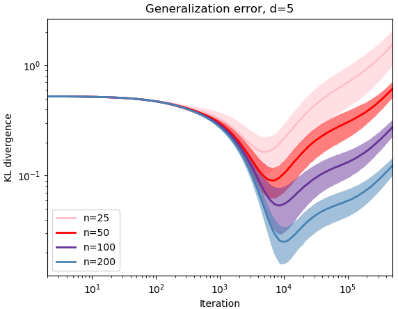
All error curves go through a rapid descent, followed by a slower but gradual ascent due to memorization. In fact, the convergence rate prior to the optimal stopping time appears to be exponential. Note that if exponential convergence indeed holds, then the generalization error estimate of Corollary 3.4 can be improved to $O(n^{-1/2}\log n)$.

Proposition 3.7 indicates that as $t\to\infty$ the model either memorizes the sample points or diverges. Our result shows that in practice we obtain memorization.

We adopt the same set-up as in Section 4.1. Since memorization occurs very slowly with SGD, we accelerate training using Adam. Figure 2 shows the result for $d=1,n=25$.

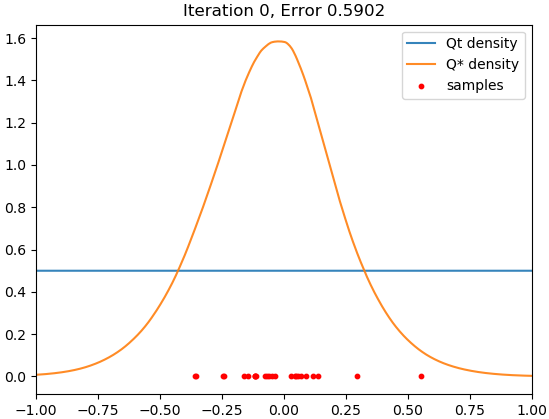
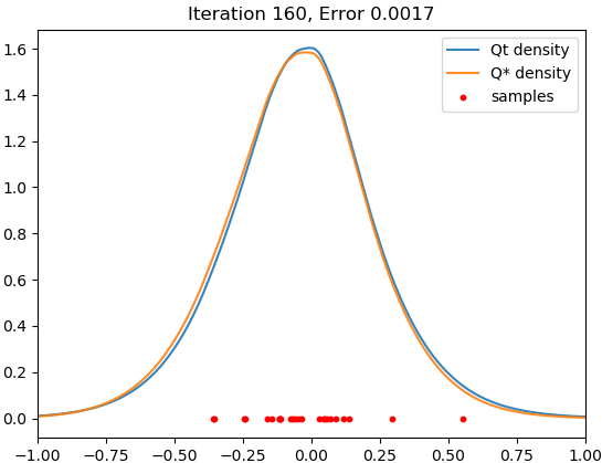
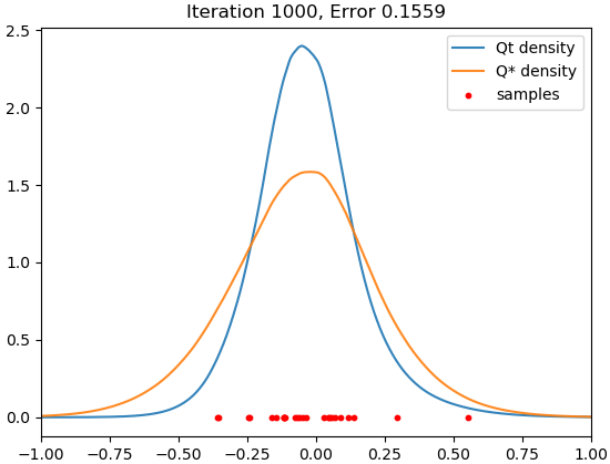
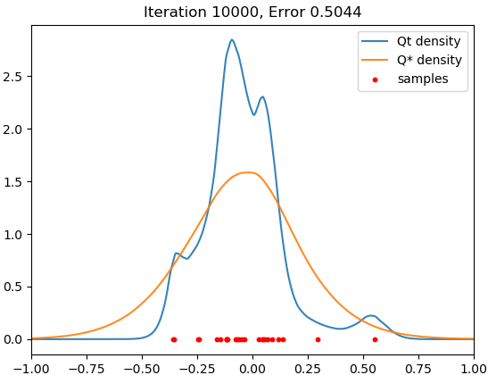
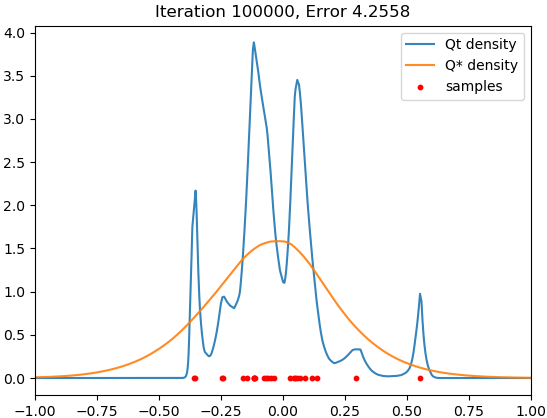
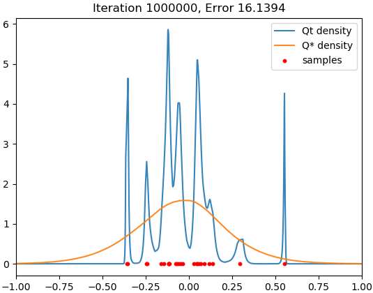
We see that there is a time interval during which the trained model closely fits the target distribution, but it eventually concentrates around the samples, and this memorization process does not seem to halt within realistic training time.

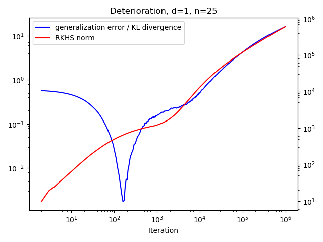
Figure 3 suggests that memorization is correlated with the growth of the function norm of the potential.

References

- [1] Arjovsky, M., and Bottou, L. Towards principled methods for training generative adversarial networks, 2017.
- [2] Arora, S., Ge, R., Liang, Y., Ma, T., and Zhang, Y. Generalization and equilibrium in generative adversarial nets (GANs). arXiv preprint arXiv:1703.00573 (2017).
- [3] Bai, Y., Ma, T., and Risteski, A. Approximability of discriminators implies diversity in GANs, 2019.
- [4] Barron, A. R., and Sheu, C.-H. Approximation of density functions by sequences of exponential families. The Annals of Statistics (1991), 1347–1369.
- [5] Bau, D., Strobelt, H., Peebles, W., Wulff, J., Zhou, B., Zhu, J.-Y., and Torralba, A. Semantic photo manipulation with a generative image prior. ACM Transactions on Graphics 38, 4 (Jul 2019), 1–11.
- [6] Bonati, L., Zhang, Y.-Y., and Parrinello, M. Neural networks-based variationally enhanced sampling. In Proceedings of the National Academy of Sciences (2019), vol. 116, pp. 17641–17647.
- [7] Brock, A., Donahue, J., and Simonyan, K. Large scale GAN training for high fidelity natural image synthesis. arXiv preprint arXiv:1809.11096 (2018).
- [8] Brown, T. B., Mann, B., Ryder, N., Subbiah, M., Kaplan, J., Dhariwal, P., Neelakantan, A., Shyam, P., Sastry, G., Askell, A., Agarwal, S., Herbert-Voss, A., Krueger, G., Henighan, T., Child, R., Ramesh, A., Ziegler, D. M., Wu, J., Winter, C., Hesse, C., Chen, M., Sigler, E., Litwin, M., Gray, S., Chess, B., Clark, J., Berner, C., McCandlish, S., Radford, A., Sutskever, I., and Amodei, D. Language models are few-shot learners, 2020.
- [9] Bubeck, S., Eldan, R., and Lehec, J. Sampling from a log-concave distribution with projected Langevin Monte Carlo. Discrete & Computational Geometry 59, 4 (2018), 757–783.
- [10] Canu, S., and Smola, A. Kernel methods and the exponential family. Neurocomputing 69, 7-9 (2006), 714–720.
- [11] Casert, C., Mills, K., Vieijra, T., Ryckebusch, J., and Tamblyn, I. Optical lattice experiments at unobserved conditions and scales through generative adversarial deep learning, 2020.
- [12] Che, T., Li, Y., Jacob, A., Bengio, Y., and Li, W. Mode regularized generative adversarial networks. arXiv preprint arXiv:1612.02136 (2016).
- [13] Chizat, L., and Bach, F. On the global convergence of gradient descent for over-parameterized models using optimal transport. In Advances in neural information processing systems (2018), pp. 3036–3046.
- [14] Donahue, J., and Simonyan, K. Large scale adversarial representation learning. In Advances in neural information processing systems (2019), pp. 10542–10552.
- [15] E, W., Ma, C., and Wang, Q. A priori estimates of the population risk for residual networks. arXiv preprint arXiv:1903.02154 1, 7 (2019).
- [16] E, W., Ma, C., Wojtowytsch, S., and Wu, L. Towards a mathematical understanding of neural network-based machine learning: what we know and what we don’t, 2020.
- [17] E, W., Ma, C., and Wu, L. A priori estimates for two-layer neural networks. arXiv preprint arXiv:1810.06397 (2018).
- [18] E, W., Ma, C., and Wu, L. Barron spaces and the compositional function spaces for neural network models. arXiv preprint arXiv:1906.08039 (2019).
- [19] E, W., Ma, C., and Wu, L. Machine learning from a continuous viewpoint. arXiv preprint arXiv:1912.12777 (2019).
- [20] E, W., Ma, C., and Wu, L. On the generalization properties of minimum-norm solutions for over-parameterized neural network models. arXiv preprint arXiv:1912.06987 (2019).
- [21] Elgammal, A., Liu, B., Elhoseiny, M., and Mazzone, M. CAN: Creative adversarial networks, generating “art” by learning about styles and deviating from style norms, 2017.
- [22] Feizi, S., Farnia, F., Ginart, T., and Tse, D. Understanding GANs in the LQG setting: Formulation, generalization and stability. IEEE Journal on Selected Areas in Information Theory 1, 1 (2020), 304–311.
- [23] Goodfellow, I., Pouget-Abadie, J., Mirza, M., Xu, B., Warde-Farley, D., Ozair, S., Courville, A., and Bengio, Y. Generative adversarial nets. In Advances in neural information processing systems (2014), pp. 2672–2680.
- [24] Gulrajani, I., Raffel, C., and Metz, L. Towards GAN benchmarks which require generalization. arXiv preprint arXiv:2001.03653 (2020).
- [25] Jewell, N. P. Mixtures of exponential distributions. Ann. Statist. 10, 2 (06 1982), 479–484.
- [26] Kiefer, J., and Wolfowitz, J. Consistency of the maximum likelihood estimator in the presence of infinitely many incidental parameters. Ann. Math. Statist. 27, 4 (12 1956), 887–906.
- [27] Lei, Q., Lee, J. D., Dimakis, A. G., and Daskalakis, C. Sgd learns one-layer networks in wgans, 2020.
- [28] Lovász, L., and Vempala, S. The geometry of logconcave functions and sampling algorithms. Random Structures & Algorithms 30, 3 (2007), 307–358.
- [29] Mao, Y., He, Q., and Zhao, X. Designing complex architectured materials with generative adversarial networks. Science Advances 6, 17 (2020).
- [30] Mei, S., Montanari, A., and Nguyen, P.-M. A mean field view of the landscape of two-layer neural networks. Proceedings of the National Academy of Sciences 115, 33 (2018), E7665–E7671.
- [31] Oord, A. v. d., Dieleman, S., Zen, H., Simonyan, K., Vinyals, O., Graves, A., Kalchbrenner, N., Senior, A., and Kavukcuoglu, K. WaveNet: A generative model for raw audio. arXiv preprint arXiv:1609.03499 (2016).
- [32] Pinkus, A. Approximation theory of the mlp model in neural networks. Acta numerica 8, 1 (1999), 143–195.
- [33] Prykhodko, O., Johansson, S. V., Kotsias, P.-C., Arús-Pous, J., Bjerrum, E. J., Engkvist, O., and Chen, H. A de novo molecular generation method using latent vector based generative adversarial network. Journal of Cheminformatics 11, 74 (Dec 2019), 1–11.
- [34] Radford, A., Metz, L., and Chintala, S. Unsupervised representation learning with deep convolutional generative adversarial networks. arXiv preprint arXiv:1511.06434 (2015).
- [35] Rahimi, A., and Recht, B. Uniform approximation of functions with random bases. In 2008 46th Annual Allerton Conference on Communication, Control, and Computing (2008), IEEE, pp. 555–561.
- [36] Redner, R. A., and Walker, H. F. Mixture densities, maximum likelihood and the em algorithm. SIAM review 26, 2 (1984), 195–239.
- [37] Roberts, G. O., and Tweedie, R. L. Exponential convergence of langevin distributions and their discrete approximations. Bernoulli 2, 4 (1996), 341–363.
- [38] Rotskoff, G. M., and Vanden-Eijden, E. Trainability and accuracy of neural networks: An interacting particle system approach. stat 1050 (2019), 30.
- [39] Russakovsky, O., Deng, J., Su, H., Krause, J., Satheesh, S., Ma, S., Huang, Z., Karpathy, A., Khosla, A., Bernstein, M., Berg, A. C., and Fei-Fei, L. Imagenet large scale visual recognition challenge, 2015.
- [40] Salimans, T., Goodfellow, I., Zaremba, W., Cheung, V., Radford, A., and Chen, X. Improved techniques for training GANs. In Advances in neural information processing systems (2016), pp. 2234–2242.
- [41] Shalev-Shwartz, S., and Ben-David, S. Understanding machine learning: From theory to algorithms. Cambridge university press, 2014.
- [42] Simon-Gabriel, C.-J., Barp, A., and Mackey, L. Metrizing weak convergence with maximum mean discrepancies, 2020.
- [43] Sriperumbudur, B., Fukumizu, K., Gretton, A., Hyvärinen, A., and Kumar, R. Density estimation in infinite dimensional exponential families. Journal of Machine Learning Research 18 (2017).
- [44] Sun, Y., Gilbert, A., and Tewari, A. On the approximation properties of random relu features. arXiv preprint arXiv:1810.04374 (2018).
- [45] Vahdat, A., and Kautz, J. NVAE: A deep hierarchical variational autoencoder. arXiv preprint arXiv:2007.03898 (2020).
- [46] Valsson, O., and Parrinello, M. Variational approach to enhanced sampling and free energy calculations. Physical review letters 113 (2014).
- [47] Wand, M. P., and Jones, M. C. Kernel smoothing. Crc Press, 1994.
- [48] Weed, J., and Bach, F. Sharp asymptotic and finite-sample rates of convergence of empirical measures in wasserstein distance. arxiv e-prints, art. arXiv preprint arXiv:1707.00087 (2017).
- [49] Wu, S., Dimakis, A. G., and Sanghavi, S. Learning distributions generated by one-layer relu networks. In Advances in Neural Information Processing Systems 32. Curran Associates, Inc., 2019, pp. 8107–8117.
- [50] Yuan, L., Kirshner, S., and Givan, R. Estimating densities with non-parametric exponential families. arXiv preprint arXiv:1206.5036 (2012).
- [51] Zhang, C., Bengio, S., Hardt, M., Recht, B., and Vinyals, O. Understanding deep learning requires rethinking generalization. arXiv preprint arXiv:1611.03530 (2016).
- [52] Zhang, L., E, W., and Wang, L. Monge-Ampère flow for generative modeling. arXiv preprint arXiv:1809.10188 (2018).
- [53] Zhang, P., Liu, Q., Zhou, D., Xu, T., and He, X. On the discrimination-generalization tradeoff in GANs. arXiv preprint arXiv:1711.02771 (2017).