Generalization despite overfitting in quantum machine learning models
Abstract
The widespread success of deep neural networks has revealed a surprise in classical machine learning: very complex models often generalize well while simultaneously overfitting training data. This phenomenon of benign overfitting has been studied for a variety of classical models with the goal of better understanding the mechanisms behind deep learning. Characterizing the phenomenon in the context of quantum machine learning might similarly improve our understanding of the relationship between overfitting, overparameterization, and generalization. In this work, we provide a characterization of benign overfitting in quantum models. To do this, we derive the behavior of a classical interpolating Fourier features models for regression on noisy signals, and show how a class of quantum models exhibits analogous features, thereby linking the structure of quantum circuits (such as data-encoding and state preparation operations) to overparameterization and overfitting in quantum models. We intuitively explain these features according to the ability of the quantum model to interpolate noisy data with locally “spiky” behavior and provide a concrete demonstration example of benign overfitting.
1 Introduction
A long-standing paradigm in machine learning is the trade-off between the complexity of a model family and the model’s ability to generalize: more expressive model classes contain better candidates to fit complex trends in data, but are also prone to overfitting noise [1, 2]. Interpolation, defined for our purposes as choosing a model with zero training error, was hence long considered bad practice [3]. The success of deep learning – machine learning in a specific regime of extremely complex model families with vast amounts of tunable parameters – seems to contradict this notion; here, consistent evidence shows that among some interpolating models, more complexity tends not to harm the generalisation performance111The fact that interpolation does not always harm generalization performance is in fact well-known for models like boosting and nearest neighbours, which are both interpolating models., a phenomenon described as “benign overfitting” [4].
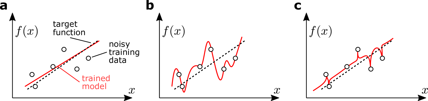
In recent years, a surge of theoretical studies have reproduced benign overfitting in simplified settings with the hope of isolating the essential ingredients of the phenomenon [4, 5]. For example, Ref. [6] showed how interpolating linear models in a high complexity regime (more dimensions than datapoints) could generalize just as well as their lower-complexity counterparts on new data, and analyzed the properties of the data that lead to the “absorption” of noise by the interpolating model without harming the model’s predictions. Ref. [7] showed that there are model classes of simple functions that change quickly in the vicinity of the noisy training data, but recover a smooth trend elsewhere in data space (see Figure 1). Such functions have also been used to train nearest neighbor models that perfectly overfit training data while generalizing well, thereby directly linking “spiking models” to benign overfitting [8]. Recent works try to recover the basic mechanism of such spiking models using the language of Fourier analysis [9, 10, 11].
In parallel to these exciting developments in the theory of deep learning, quantum computing researchers have proposed families of parametrised quantum algorithms as model classes for machine learning (e.g. Ref. [12]). These quantum models can be optimised similarly to neural networks [13, 14] and have interesting parallels to kernel methods [15, 16] and generative models [17, 18]. Although researchers have taken some first steps to study the expressivity [19, 20, 21, 22], trainability [23, 24] and generalisation [25, 26, 27, 28] of quantum models, we still know relatively little about their behaviour. In particular, the interplay of overparametrisation, interpolation, and generalisation that seems so important for deep learning is yet largely unexplored.
In this paper we develop a simplified framework in which questions of overfitting in quantum machine learning can be investigated. Essentially, we exploit the observation that quantum models can often be described in terms of Fourier series where well-defined components of the quantum circuit influence the selection of Fourier modes and their respective Fourier coefficients [29, 30, 31]. We link this description to the analysis of spiking models and benign overfitting by building on prior works analyzing these phenomena using Fourier methods. In this approach, the complexity of a model is related to the number of Fourier modes that its Fourier series representation consists of, and overparametrised model classes have more modes than needed to interpolate the training data (i.e., to have zero training error). After deriving the generalization error for such model classes these “superfluous” modes lead to spiking models, which have large oscillations around the training data while keeping a smooth trend everywhere else. However, large numbers of modes can also harm the recovery of an underlying signal, and we therefore balance this trade-off to produce an explicit example of benign overfitting in a quantum machine learning model.
The mathematical link described above allows us to probe the impact of important design choices for a simplified class of quantum models on this trade-off. For example, we find why a measure of redundancy in the spectrum of the Hamiltonian that defines standard data encoding strategies strongly influences this balance; in fact to an extent that is difficult to counterbalance by other design choices of the circuit.
The remainder of the paper proceeds as follows. We will first review the classical Fourier framework for the study of interpolating models and develop explicit formulae for the error in these models to produce a basic example of benign overfitting (Sec. 2). We will then construct a quantum model with analogous components to the classical model, and demonstrate how each of these components is related to the structure of the corresponding quantum circuit and measurement (Sec. 3). We then analyze specific cases that give rise to “spikiness” and benign overfitting in these quantum models (Sec. 3.2).
2 Interpolating models in the Fourier framework
In this section we will provide the essential tools to probe the phenomenon of overparametrized models that exhibit the spiking behaviour from Figure 1 using the language of Fourier series. We will review and formalize the problem setting and several examples from Refs. [9, 10, 11], before extending their framework by incorporating standard results from linear regression to derive closed-form error behavior and examples of benign overfitting.
2.1 Setting up the learning problem
We are interested in functions defined on a finite interval that may be written in terms of a linear combination of Fourier basis functions or modes (each describing a complex sinusoid with integer-valued frequency ) weighted by their corresponding Fourier coefficients :
| (1) |
We restrict our attention to well-behaved functions that are sufficiently smooth and continuous to be expressed in this form. We will now set up a simple learning problem whose basic components – the model and target function to be learned – can be expressed as Fourier series with only few non-zero coefficients, and define concepts such as overparametrization and interpolation.
Consider a machine learning problem in which data is generated by a target function of the form
| (2) |
which only contains frequencies in the discrete, integer-valued spectrum
| (3) |
for some odd integer . We call functions of this form band-limited with bandwidth (that is, for all frequencies ). The bandwidth limits the complexity of a function, and will therefore be important for exploring scenarios where a complex model is used to overfit a less complex target function. We are provided with noisy samples of the target function evaluated at points spaced uniformly on interval (we will assume input data has been rescaled to without loss of generality), where and we require to be odd for simplicity.
The model class we consider likewise contains band-limited Fourier series, and since we are interested in interpolating models, we always assume that they have enough modes to interpolate the noisy training data, namely:
| (4) | ||||
Similarly to Eq. (3) we define the spectrum
| (5) |
Following Ref. [9], this model class has two components: The set of weighted Fourier basis functions describe a feature map applied to for some set of feature weights , while the trainable weights are optimized to ensure that interpolates the data. The theory of trigonometric polynomial interpolation [32] ensures that can always interpolate the training data for some choice of trainable weights under these conditions. In the following, we will therefore usually consider the as being determined by the data and interpolation condition, while the serve as our “turning knobs” to create different settings in which to study spiking properties and benign overfitting. We call the model class described in Eq. (4) overparameterized when the degree of the Fourier series is much larger than the degree of the target function, , in which case the model has many more frequencies available to perform fitting than there are present in the underlying signal to fit.
Note that one can rewrite the Fourier series of Eq. (4) in a linear form
| (6) |
where
| (7) | ||||
| (8) |
From this perspective, optimizing amounts to learning trainable weights by performing regression on observations sampled from a random Fourier features model [33] for which and are precisely the eigenvalues and eigenfunctions of a shift-invariant kernel [34].
To complete the problem setup, we have to impose one more constraint. Consider that with frequency and uniformly spaced points is equal to for any choice of alias frequency . The presence of these aliases means that the model class described in Eq. (6) contains many interpolating solutions in the overparameterized regime. Motivated by prior work exploring benign overfitting for linear features [6], Fourier features [9, 35], and other nonlinear features [36, 37], we will study the minimum- norm interpolating solution,
| (9) |
Minimizing the norm is a typical choice for imposing a penalty on complex functions (regularization) in the underparameterized regime, though we will see that this intuition does not carry over to the overparameterized regime. The remainder of this section will explore how this learning problem results in a trade-off in interpolating Fourier models: Overparameterization introduces alias frequencies that increase the error in fitting simple target functions but can also reduce error by absorbing noise into high-frequency modes with spiking behavior.
2.2 Two extreme cases to understand generalization
To better understand the trade-off that overparametrization – or in our case, a much larger number of Fourier modes than needed to interpolate the data – introduces between fitting noise and generalization error, we revisit two extreme cases explored in Ref. [9], involving a pure-noise signal and a noiseless signal.
Case 1: Noise only
The first case demonstrates how alias modes can help to fit noise without disturbing the (here trivial) signal. We set and consider observations of zero-mean noise with known variance . After making uniformly spaced observations, we compute the discrete Fourier transform of the observations as the sequence of values satisfying
| (10) |
which characterizes the frequency content of the noisy signal that can be captured and learned from using only evenly spaced samples. Suppose that the degree of the model (controlling the model complexity) is given by for some even integer and that for every mode, so that there are exactly equally-weighted aliases for each frequency in the spectrum of the Fourier series for . Then the optimal (i.e., the minimum -norm, interpolating) trainable weight vector has entries
| (11) |
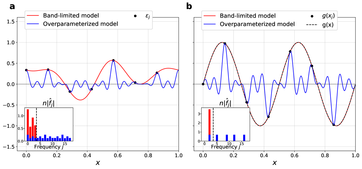
for , with all other entries being zero (see Appendix A.2). From Eq. (11), the minimum- solution distributes noise Fourier coefficients evenly into many alias frequencies , while enforcing that the sum of trainable weights for all of these aliases is to guarantee interpolation. As shown in Figure 2, the higher-frequency aliases suppress the optimal model to near-zero at every point away from the interpolated points, resulting in a test error of that decreases monotonically with the complexity of the model. As increases, the optimal model remains close to the true signal while becoming “spiky” near the noisy samples. By conforming to the true signal everywhere except in the vicinity of noise, this behavior embodies the mechanism of how overparameterized models can absorb noise into high frequency modes. In this case the generalization error, measuring how close the model is to the target function on average, decreases with increasing complexity of the model class.
Case 2: Signal only
While the above case shows how overparametrization can help to absorb noise to reduce error without harming the signal, the second case will illustrate how alias frequencies in the overparameterized model can harm the model’s ability to learn the target function. To demonstrate this, we now consider a noiseless, single-mode signal of frequency . The data is hence of the form
| (12) |
Once again we choose and for simplicity we assume an unweighted model, for . By orthonormality of Fourier basis functions, the interpolation condition requires that only the modes of the model with integer multiples of the frequency are retained. The interpolation constraint can then be rewritten as
| (13) |
The choice of trainable weights that satisfy Eq. (13) while minimizing -norm is
| (14) |
for and otherwise (see Appendix A.2). Eq. (13) distributes the Fourier coefficient among the trainable weights corresponding to frequencies . Therefore, minimizing in this case “bleeds” the target function into higher frequency aliases and results in the opposite effect compared to fitting a noisy signal (see Fig. 2b): The generalization error of the overparameterized model now increases with the number of aliases and the complexity of the model harms its ability to fit a noiseless target function.
In order to recover a trade-off in generalization error for more general cases, we will need to consider more interesting distributions of feature weights (instead of ) that provide finer control over fitting the target function with low-frequency modes while spiking in the vicinity of noise with high-frequency aliases.
2.3 Generalization trade-offs and benign overfitting
The opposing effects of higher-frequency modes in overparameterized models in the cases discussed above hint at a trade-off in model performance that depends on the underlying signal and the feature weights of the Fourier feature map. Returning to the more general case of input samples , in Appendix A we show that the task of fitting uniformly spaced samples using weighted Fourier features may be transformed into a linear regression problem, thereby generalizing the results of [9] to derive the following general solution to the minimum- interpolating problem of Eq. (9):
| (15) |
where is the discrete Fourier transform of and , where
| (16) |
denotes the set of alias frequencies of appearing in the overparameterized model with spectrum . The optimal model is then expressed as
| (17) |
Recalling that our model is trained on noisy samples of the target function , we are interested in the squared error of the model averaged over (noisy) samples over the input domain,
| (18) |
and we call the generalization error of , as it captures the behavior of with respect to over the entire input domain instead of just the uniformly spaced training points . In Appendix A we derive
| (19) |
We use this generalization error now to explore two interesting behaviors of the interpolating model in our setting: The tradeoff between noise absorption and signal recovery exemplified by the cases in Sec. 2.2, and the ability of an overparameterized Fourier features model to benignly overfit the training data.
The first behavior involves a trade-off in the generalization error between absorbing noise (reducing var) and capturing the target function signal (reducing ) that recovers and generalizes the behavior of the two cases in Sec. 2.2. This trade-off is controlled by three components: The noise variance , the input signal Fourier coefficients , and the distribution of feature weights . As described in the two cases above, when (signal only) the variance term var vanishes and the model is biased for any choice of nonzero where . Conversely, when (noise only) the bias term vanishes, and the variance term is minimized by choosing uniform for all .
The second interesting behavior occurs when the generalization error of the overparameterized model decreases at a nearly optimal rate as the number of samples increases, known as benign overfitting. Prior work on benign overfitting in linear regression studied scenarios where the distribution of input data varied with the dimensionality of data and size of the training set in such a way that the excess generalization error of the overparameterized model (compared to a simple model) vanished [6]. However, since the dimensionality of the input data for our model is fixed, we instead consider sequences of feature weights that vary with respect to the problem parameters (, , ) in a way that results in and var vanishing as . In this case, by fitting an increasing number of samples using such a sequence of feature weights, the overparameterized model both perfectly fits the training data and generalizes well for unseen test points, and therefore exhibits benign overfitting.
These behaviors are exemplified by a straightforward choice of feature weights that incorporate some prior knowledge of the spectrum available to the target function . For all , let for some positive and normalize the feature weights so that . We show in Appendix A.3.1 that the error terms of scale as
| var | (20) | |||
| (21) |
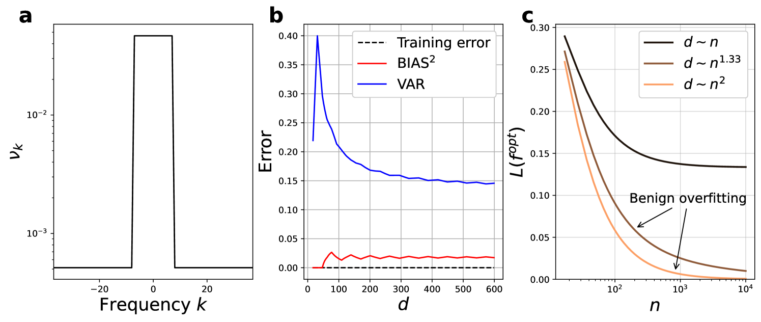
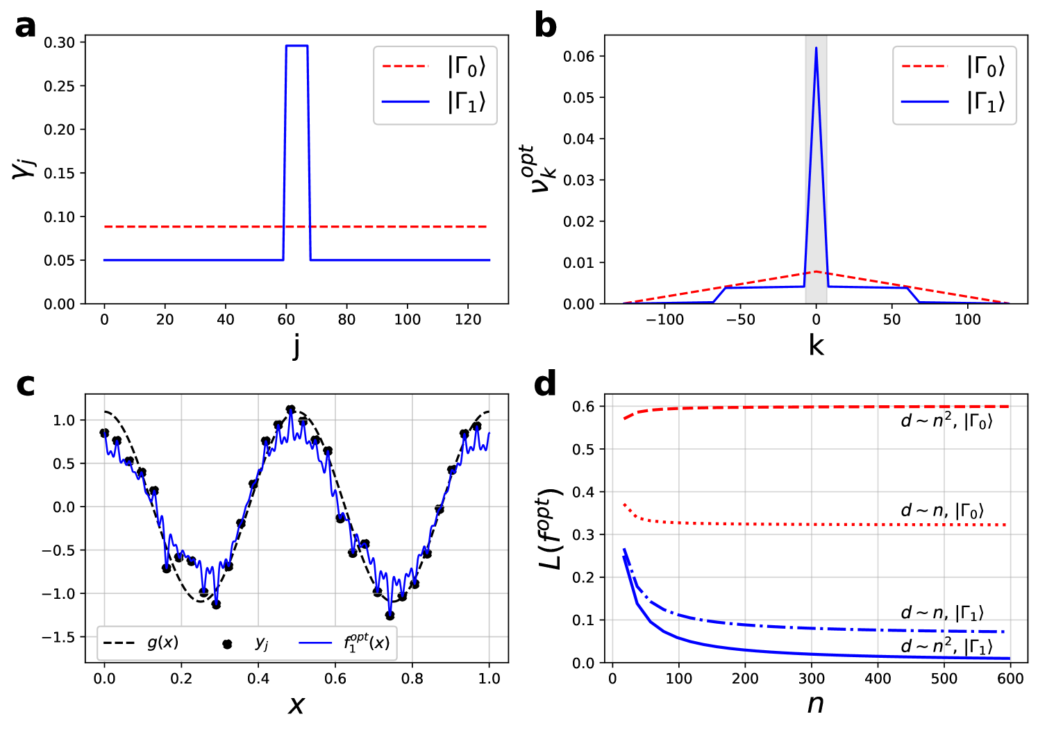
Thus, as long as the dimension of the overparameterized Fourier features model grows strictly faster than (i.e., ), the model exhibits benign overfitting. In Appendix A.3.2 we demonstrate how this simple example actually captures the mechanisms of benign overfitting for much more general choices of feature weights. Fig. 3 summarizes this behavior and provides an example of the bias-variance tradeoff that occurs for overparameterized models. In particular, Fig. 3a exemplifies the setting in which benign overfitting occurs, wherein the feature weights of the Fourier features model are strongly concentrated over frequencies in but extend over a large range of alias frequencies for each .
The generalization behavior described here is fundamentally different from many generalization guarantees typically found in statistical learning theory. While prior work has derived guarantees for the generalization of quantum models by constructing bounds on the complexity of the model class [25], Eqs. 20-21 demonstrate that generalization may occur as the complexity (i.e. dimension) of a model grows arbitrarily large.
So far, we have reviewed the Fourier perspective on fitting periodic functions in a classical setting and extended the analysis to characterize benign overfitting. However, if we can link the basic components of quantum models to the terms appearing in the error of Eq. (19), then we will be able to study a similar trade-off in the error of overparameterized quantum models and the conditions necessary for benign overfitting. The remainder of this work is devoted to showing that analogous mechanisms exist in certain quantum machine learning models, and to studying the choices of feature weights for which quantum models can exhibit tradeoffs in generalization error and benign overfitting.
3 Benign overfitting in single-layer quantum models
In the previous section we have seen that the feature weights balance the trade-off between absorbing the noise and hurting the signal of overparametrized models. To understand how different design choices of quantum models impact this balance, we need to link their mathematical structure to the model class defined in Eq. (4), and in particular to the feature weights, which is what we do now.
The type of quantum models we consider here are simplified versions of parametrized quantum classifiers (also known as quantum neural networks) that have been heavily investigated in recent years [13, 38, 39]. They are represented by quantum circuits that consist of two steps: first, we encode a datapoint into the state of the quantum system by applying a -dimensional unitary operator , and then we measure the expectation value of some -dimensional (Hermitian) observable . This gives rise to a general class of quantum models of the form
| (22) |
To simplify the analysis, we will consider a quantum circuit that consists of a data-independent unitary and a diagonal data-encoding unitary generated by a -dimensional Hermitian operator ,
| (23) |
which includes a large class of quantum models commonly studied but excludes schemes involving data re-uploading [40, 41]. Defining , the output of this quantum model becomes
| (24) |
where can be treated as an arbitrary input quantum state. We call the corresponding quantum circuit for this model single-layer in the sense that it contains a single diagonal data-encoding layer in which all data-dependent circuit operations could theoretically be executed simultaneously (though in general the operation and measurement may require significant depth to implement).
Applying insights from Refs. [29, 30], quantum models of this form can be expressed in terms of a Fourier series
| (25) |
where the spectrum as well as the partitions depend on the eigenspectrum of the data-encoding Hamiltonian :
| (26) | ||||
| (27) |
Comparing Eq. (25) to Eq. (4) we see that that the quantum model may be expressed as a linear combination of weighted Fourier modes, but it is not yet clear how the input state and the trainable observable of the quantum model correspond to feature weights for each Fourier mode. To reveal this correspondence, we will need to first find the minimum-norm interpolating observable that solves the optimization problem
| (28) |
where denotes the Frobenius norm of . Solving Eq. (28) is analogous to the minimization the norm of in the classical optimization problem of Eq. (9), and serves a role similar to regularization commonly applied to quantum models by introducing a penalty term proportional to [26, 42, 43]. In Appendix B we prove that subject to the condition that , the minimum- interpolating observable that solves Eq. (28) is given as
| (29) |
for all , and the corresponding optimal quantum model is
| (30) |
where denotes the set of aliases of appearing in from Eq. (16). By comparison to the optimal classical model of Eq. (17) we have identified the feature weights of the optimized quantum model as
| (31) |
Interestingly, while there was initially no clear way to separate the building blocks of the quantum model in Eq. (25) into trainable weights and feature weights , this separation has now appeared after solving for the optimal observable . Furthermore, the optimal quantum model depends on and is independent of phases associated with amplitudes (an effect that stems from using only a single data-encoding layer in the quantum model).
From Eq. (31) it is clear that the partitions of Eq. (27) arising from the choice of data-encoding unitary have a strong relationship with the feature weights of the quantum model. We will now consider a simplified quantum model to highlight this relationship, thereby identifying a tradeoff between noise absorption and target signal recovery and the possibility of observing benign overfitting in quantum models.
3.1 Simplified quantum model
To explicitly highlight the role of in controlling the feature weights of the optimized quantum model, we will now simplify the model by using an equal superposition input state and by restricting the set of observables considered during optimization. If we fix every entry of the observable with respect to elements in a partition to be proportional to some complex constant :
| (32) |
then we can simplify the quantum model of Eq. (25) to
| (33) |
Comparing Eq. (33) to Eq. (4) we identify a direct correspondence between the trainable weights in the classical model with , as well as a correspondence between the feature weights and the the degeneracy of the quantum model. Making the substitutions , , one can verify that for this restricted choice of and so the solution to the optimization of Eq. (28) is essentially the same as that of the classical problem in Eq. (15).
The crucial property of the simplified model is that the degeneracy – and hence the combinatorial structure introduced by the data encoding Hamiltonian’s eigenvalues – completely controls the trade-off in the generalization error (Eq. (19)). We can hence study different types of partitions to show a direct effect of the data-encoding unitary on the fitting and generalization error behaviors for this simplified, overparameterized quantum model.
To study these behaviors we will now consider specific families of which we call encoding strategies since the choice of completely determines how the data is encoded into the quantum model. While and may be computed for an arbitrary using brute-force combinatorics, some encoding strategies lead to particularly simple solutions. We have derived a few such examples of simple degeneracies and spectra for different encoding strategies in Appendix C and present the results in Table 1. These choices highlight the extreme variation in resulting from minor changes to , for example for the “Hamming” encoding strategy compared to for the “Ternary” encoding strategy. These examples also highlight the limitations in constructing Hamiltonians with specific properties such as uniform or evenly-spaced frequencies in .
| Encoding strategy | Hamiltonian example | Degeneracy | Spectrum | |
| Hamming | ||||
| Binary | ||||
| Ternary | ||||
| Golomb | varies |
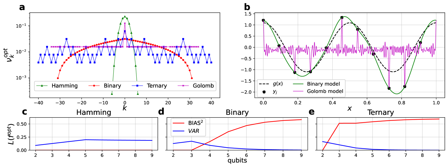
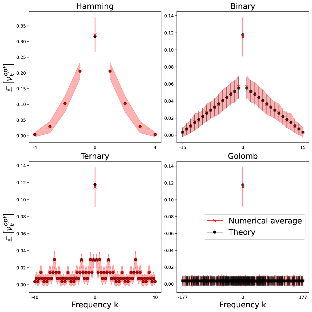
Since the feature weights of the Fourier modes are fixed by the choice of the data-encoding unitary, we can understand a choice of as providing a structural bias of a quantum model towards different overfitting behaviors, and conversely the choices of feature weights available to quantum models are limited and are particular to the structure of the associated quantum circuit. Figure 4 shows distributions for feature weights arising from the example encoding strategies presented in Table 2, and demonstrates a broad connection between the degeneracies of the model (giving rise to feature weights ) and the generalization error .
3.2 Trainable unitaries reweight the general quantum model
We now return to the general quantum model of Eq. (25) to understand how different choices of the state preparation unitary (giving rise to input state ) affect the feature weights of the general quantum model, thereby influencing benign overfitting of the target function. While Eq. (31) differs from the correspondence that we observed for the simplified quantum model, we see that the feature weights of the optimal quantum model still depend heavily on the degeneracies . For instance, the average with respect to Haar-random -dimensional input states is proportional to whenever :
| (34) |
where denotes the Kronecker delta. Furthermore, in Appendix B we observe that the variance of around its average tends to be small for encoding strategies considered in this work, for instance scaling like for the Binary encoding strategy and for the Golomb encoding strategy. This demonstrates that the feature weights of generic quantum models (i.e., ones for which is randomly sampled) will be dominated by the degeneracy introduced by the data-encoding operation .
Despite the behavior of being dominated by in an average sense, there are specific choices of for which the feature weights deviate significantly from this average. We will now use one such choice of to provide a concrete example of an interpolating quantum model that exhibits benign overfitting. Suppose we choose such that the elements of are given by
| (35) |
for , and some integers and amplitudes subject to normalization. We show that given a band-limited target function with access to spectrum , there is a specific choice of dependent on and for which the interpolating quantum model of Eq. (30) also benefits from vanishing generalization error in the limit of many samples, namely we show in Appendix D that
| (36) |
Thus, by perfectly fitting the training data and exhibiting good generalization in the limit, the quantum model exhibits benign overfitting. This behavior is outlined in Figure 5, which highlights the role that plays in concentrating the feature weights within the spectrum of while preserving a long tail that provides the model with low-variance “spiky” behavior in the vicinity of noisy samples. In contrast, the feature weights for the Binary encoding strategy with a uniform input state has little support on and resulting in a large bias error.
The above discussion shows how the input state amplitudes provide additional degrees of freedom with which the feature weights can be tuned in order to modify the generalization behavior of the interpolating quantum model, and to exhibit benign overfitting in particular. It is therefore worthwhile to consider what other kinds of feature weights might be prepared by some choice of input state . We may use simple counting arguments to demonstrate the restrictions in designing particular distributions of feature weights. Suppose we define containing the positive frequencies of a quantum model. Then the introduction of an arbitrary input state provides us with free parameters with which to tune -many terms in the distribution of (subject to and ). Clearly, there are distributions of feature weights that can not be achieved for models where .
Conversely, the condition does not necessarily mean that we can thoroughly explore the space of possible feature weights by modifying the input state . For example, consider the Hamming encoding strategy for which the number of free parameters controlling the distribution of feature weights is , which is exponentially smaller the number of parameters in . While this might suggest significant freedom in adjusting , the opposite is true: For any choice of input state , there is another state of the form
| (37) |
that achieves exactly the same distribution of feature weights . In Eq. (37), describes a uniform superposition over all computational basis state bitstrings with weight , and so the distribution of actually only depends on real parameters , , and the feature weights are invariant under any operations in that preserve (see Appendix B). An example of such operations are the particle-conserving unitaries well-known in quantum chemistry, which act to preserve the number of set bits (i.e., the Hamming weight) when each bit represents a mode occupied by a particle in second quantization [46, 47]. This example demonstrates how symmetry in the data-encoding Hamiltonian (e.g. Refs. [48, 49]) can have a profound influence on the ability to prepare specific distributions of feature weights , and consequently affect the generalization and overparameterization behavior of the associated quantum models.
4 Conclusion
In this work we have taken a first step towards characterizing the phenomenon of benign overfitting in a quantum machine learning setting. We derived the error for an overparameterized Fourier features model that interpolates the (noisy) input signal with minimum -norm trainable weights and connected the feature weights associated with each Fourier mode to a trade-off in the generalization error of the model. We then demonstrated an analogous simplified quantum model for which the feature weights are induced by the choice of data-encoding unitary . Finally, we discussed how introducing an arbitrary state-preparation unitary gives rise to effective feature weights in the optimized general quantum model, presenting the possibility of connecting and to benign overfitting in more general quantum models.
Our discussion of interpolating quantum models presents an interpretation of overparameterization (i.e., the size of the model spectrum ) that departs from other measures of quantum circuit complexity discussed in the literature [19, 50, 51], as even the simplified quantum models studied here are able to interpolate training data using a fixed circuit and optimized measurements. We also reemphasize that – unlike much of the quantum machine learning literature – we do not consider a setting where the model is optimized with respect to a trainable circuit, as the model of Eq. (30) is constructed to exhibit zero training error (and can therefore not be improved via optimization). Finding the input state that will result in a specific distribution of feature weights generally requires solving a -dimensional system of equations that are second order in many real parameters (i.e., inverting the map of the form in Eq. (31)) or otherwise performing a variational optimization that will likely fail due to the familiar phenomenon of barren plateaus [23, 24, 52, 53].
While we have shown an example of benign overfitting by a quantum model in a relatively restricted context, future work may lead to more general characterizations of this phenomenon. Similar behavior likely exists for quantum kernel methods and may complement existing studies on these methods’ generalization power [54]. An exciting possibility would be to demonstrate benign overfitting in quantum models trained on distributions of quantum states which are hard to learn classically [55, 56], thereby extending the growing body of statistical learning theory for quantum learning algorithms [27, 28, 57].
5 Code availability
Code to reproduce the figures and analysis is available at the following repository: https://github.com/peterse/benign-overfitting-quantum.
6 Acknowledgements
The authors thank Nathan Killoran, Achim Kempf, Angus Lowe, and Joseph Bowles for helpful feedback. This work was supported by Mitacs through the Mitacs Accelerate program. Research at Perimeter Institute is supported in part by the Government of Canada through the Department of Innovation, Science and Economic Development and by the Province of Ontario through the Ministry of Colleges and Universities. Circuit simulations were performed in PennyLane [58].
References
- [1] Michael A Nielsen. “Neural networks and deep learning”. Determination Press. (2015). url: http://neuralnetworksanddeeplearning.com/.
- [2] Stuart Geman, Elie Bienenstock, and René Doursat. “Neural networks and the bias/variance dilemma”. Neural Comput. 4, 1–58 (1992).
- [3] Trevor Hastie, Robert Tibshirani, Jerome H Friedman, and Jerome H Friedman. “The elements of statistical learning: data mining, inference, and prediction”. Volume 2. Springer. (2009).
- [4] Peter L. Bartlett, Andrea Montanari, and Alexander Rakhlin. “Deep learning: a statistical viewpoint”. Acta Numerica 30, 87–201 (2021).
- [5] Mikhail Belkin. “Fit without fear: remarkable mathematical phenomena of deep learning through the prism of interpolation”. Acta Numerica 30, 203–248 (2021).
- [6] Peter L. Bartlett, Philip M. Long, Gábor Lugosi, and Alexander Tsigler. “Benign overfitting in linear regression”. Proc. Natl. Acad. Sci. 117, 30063–30070 (2020).
- [7] Mikhail Belkin, Daniel Hsu, Siyuan Ma, and Soumik Mandal. “Reconciling modern machine-learning practice and the classical bias-variance trade-off”. Proc. Natl. Acad. Sci. 116, 15849–15854 (2019).
- [8] Mikhail Belkin, Alexander Rakhlin, and Alexandre B. Tsybakov. “Does data interpolation contradict statistical optimality?”. In Proceedings of Machine Learning Research. Volume 89, pages 1611–1619. PMLR (2019). url: https://proceedings.mlr.press/v89/belkin19a.html.
- [9] Vidya Muthukumar, Kailas Vodrahalli, Vignesh Subramanian, and Anant Sahai. “Harmless interpolation of noisy data in regression”. IEEE Journal on Selected Areas in Information Theory 1, 67–83 (2020).
- [10] Vidya Muthukumar, Adhyyan Narang, Vignesh Subramanian, Mikhail Belkin, Daniel Hsu, and Anant Sahai. “Classification vs regression in overparameterized regimes: Does the loss function matter?”. J. Mach. Learn. Res. 22, 1–69 (2021). url: http://jmlr.org/papers/v22/20-603.html.
- [11] Yehuda Dar, Vidya Muthukumar, and Richard G. Baraniuk. “A farewell to the bias-variance tradeoff? an overview of the theory of overparameterized machine learning” (2021). arXiv:2109.02355.
- [12] Marcello Benedetti, Erika Lloyd, Stefan Sack, and Mattia Fiorentini. “Parameterized quantum circuits as machine learning models”. Quantum Sci. Technol. 4, 043001 (2019).
- [13] K. Mitarai, M. Negoro, M. Kitagawa, and K. Fujii. “Quantum circuit learning”. Phys. Rev. A 98, 032309 (2018).
- [14] Maria Schuld, Ville Bergholm, Christian Gogolin, Josh Izaac, and Nathan Killoran. “Evaluating analytic gradients on quantum hardware”. Phys. Rev. A 99, 032331 (2019).
- [15] Maria Schuld and Nathan Killoran. “Quantum machine learning in feature hilbert spaces”. Phys. Rev. Lett. 122, 040504 (2019).
- [16] Vojtěch Havlíček, Antonio D. Córcoles, Kristan Temme, Aram W. Harrow, Abhinav Kandala, Jerry M. Chow, and Jay M. Gambetta. “Supervised learning with quantum-enhanced feature spaces”. Nature 567, 209–212 (2019).
- [17] Seth Lloyd and Christian Weedbrook. “Quantum generative adversarial learning”. Phys. Rev. Lett. 121, 040502 (2018).
- [18] Pierre-Luc Dallaire-Demers and Nathan Killoran. “Quantum generative adversarial networks”. Phys. Rev. A 98, 012324 (2018).
- [19] Amira Abbas, David Sutter, Christa Zoufal, Aurelien Lucchi, Alessio Figalli, and Stefan Woerner. “The power of quantum neural networks”. Nat. Comput. Sci. 1, 403–409 (2021).
- [20] Logan G. Wright and Peter L. McMahon. “The capacity of quantum neural networks”. In 2020 Conference on Lasers and Electro-Optics (CLEO). Pages 1–2. (2020). url: https://ieeexplore.ieee.org/document/9193529.
- [21] Sukin Sim, Peter D. Johnson, and Alán Aspuru-Guzik. “Expressibility and entangling capability of parameterized quantum circuits for hybrid quantum-classical algorithms”. Adv. Quantum Technol. 2, 1900070 (2019).
- [22] Thomas Hubregtsen, Josef Pichlmeier, Patrick Stecher, and Koen Bertels. “Evaluation of parameterized quantum circuits: on the relation between classification accuracy, expressibility and entangling capability”. Quantum Mach. Intell. 3, 1 (2021).
- [23] Jarrod R McClean, Sergio Boixo, Vadim N Smelyanskiy, Ryan Babbush, and Hartmut Neven. “Barren plateaus in quantum neural network training landscapes”. Nat. Commun. 9, 4812 (2018).
- [24] Marco Cerezo, Akira Sone, Tyler Volkoff, Lukasz Cincio, and Patrick J Coles. “Cost function dependent barren plateaus in shallow parametrized quantum circuits”. Nat. Commun. 12, 1791 (2021).
- [25] Matthias C. Caro, Elies Gil-Fuster, Johannes Jakob Meyer, Jens Eisert, and Ryan Sweke. “Encoding-dependent generalization bounds for parametrized quantum circuits”. Quantum 5, 582 (2021).
- [26] Hsin-Yuan Huang, Michael Broughton, Masoud Mohseni, Ryan Babbush, Sergio Boixo, Hartmut Neven, and Jarrod R McClean. “Power of data in quantum machine learning”. Nat. Commun. 12, 2631 (2021).
- [27] Matthias C. Caro, Hsin-Yuan Huang, M. Cerezo, Kunal Sharma, Andrew Sornborger, Lukasz Cincio, and Patrick J. Coles. “Generalization in quantum machine learning from few training data”. Nat. Commun. 13, 4919 (2022).
- [28] Leonardo Banchi, Jason Pereira, and Stefano Pirandola. “Generalization in quantum machine learning: A quantum information standpoint”. PRX Quantum 2, 040321 (2021).
- [29] Francisco Javier Gil Vidal and Dirk Oliver Theis. “Input redundancy for parameterized quantum circuits”. Front. Phys. 8, 297 (2020).
- [30] Maria Schuld, Ryan Sweke, and Johannes Jakob Meyer. “Effect of data encoding on the expressive power of variational quantum-machine-learning models”. Phys. Rev. A 103, 032430 (2021).
- [31] David Wierichs, Josh Izaac, Cody Wang, and Cedric Yen-Yu Lin. “General parameter-shift rules for quantum gradients”. Quantum 6, 677 (2022).
- [32] Kendall E Atkinson. “An introduction to numerical analysis”. John Wiley & Sons. (2008).
- [33] Ali Rahimi and Benjamin Recht. “Random features for large-scale kernel machines”. In Advances in Neural Information Processing Systems. Volume 20. (2007). url: https://papers.nips.cc/paper_files/paper/2007/hash/013a006f03dbc5392effeb8f18fda755-Abstract.html.
- [34] Walter Rudin. “The basic theorems of fourier analysis”. John Wiley & Sons, Ltd. (1990).
- [35] Song Mei and Andrea Montanari. “The generalization error of random features regression: Precise asymptotics and the double descent curve”. Commun. Pure Appl. Math. 75, 667–766 (2022).
- [36] Trevor Hastie, Andrea Montanari, Saharon Rosset, and Ryan J. Tibshirani. “Surprises in high-dimensional ridgeless least squares interpolation”. Ann. Stat. 50, 949 – 986 (2022).
- [37] Tengyuan Liang, Alexander Rakhlin, and Xiyu Zhai. “On the multiple descent of minimum-norm interpolants and restricted lower isometry of kernels”. In Proceedings of Machine Learning Research. Volume 125, pages 1–29. PMLR (2020). url: http://proceedings.mlr.press/v125/liang20a.html.
- [38] Edward Farhi and Hartmut Neven. “Classification with quantum neural networks on near term processors” (2018). arXiv:1802.06002.
- [39] Maria Schuld, Alex Bocharov, Krysta M. Svore, and Nathan Wiebe. “Circuit-centric quantum classifiers”. Phys. Rev. A 101, 032308 (2020).
- [40] Adrián Pérez-Salinas, Alba Cervera-Lierta, Elies Gil-Fuster, and José I. Latorre. “Data re-uploading for a universal quantum classifier”. Quantum 4, 226 (2020).
- [41] Sofiene Jerbi, Lukas J Fiderer, Hendrik Poulsen Nautrup, Jonas M Kübler, Hans J Briegel, and Vedran Dunjko. “Quantum machine learning beyond kernel methods”. Nat. Commun. 14, 517 (2023).
- [42] Casper Gyurik, Dyon Vreumingen, van, and Vedran Dunjko. “Structural risk minimization for quantum linear classifiers”. Quantum 7, 893 (2023).
- [43] Maria Schuld. “Supervised quantum machine learning models are kernel methods” (2021). arXiv:2101.11020.
- [44] S. Shin, Y. S. Teo, and H. Jeong. “Exponential data encoding for quantum supervised learning”. Phys. Rev. A 107, 012422 (2023).
- [45] Sophie Piccard. “Sur les ensembles de distances des ensembles de points d’un espace euclidien.”. Memoires de l’Universite de Neuchatel. Secretariat de l’Universite. (1939).
- [46] Dave Wecker, Matthew B. Hastings, Nathan Wiebe, Bryan K. Clark, Chetan Nayak, and Matthias Troyer. “Solving strongly correlated electron models on a quantum computer”. Phys. Rev. A 92, 062318 (2015).
- [47] Ian D. Kivlichan, Jarrod McClean, Nathan Wiebe, Craig Gidney, Alán Aspuru-Guzik, Garnet Kin-Lic Chan, and Ryan Babbush. “Quantum simulation of electronic structure with linear depth and connectivity”. Phys. Rev. Lett. 120, 110501 (2018).
- [48] Martín Larocca, Frédéric Sauvage, Faris M. Sbahi, Guillaume Verdon, Patrick J. Coles, and M. Cerezo. “Group-invariant quantum machine learning”. PRX Quantum 3, 030341 (2022).
- [49] Johannes Jakob Meyer, Marian Mularski, Elies Gil-Fuster, Antonio Anna Mele, Francesco Arzani, Alissa Wilms, and Jens Eisert. “Exploiting symmetry in variational quantum machine learning”. PRX Quantum 4, 010328 (2023).
- [50] Martin Larocca, Nathan Ju, Diego García-Martín, Patrick J Coles, and Marco Cerezo. “Theory of overparametrization in quantum neural networks”. Nat. Comput. Sci. 3, 542–551 (2023).
- [51] Yuxuan Du, Min-Hsiu Hsieh, Tongliang Liu, and Dacheng Tao. “Expressive power of parametrized quantum circuits”. Phys. Rev. Res. 2, 033125 (2020).
- [52] Zoë Holmes, Kunal Sharma, M. Cerezo, and Patrick J. Coles. “Connecting ansatz expressibility to gradient magnitudes and barren plateaus”. PRX Quantum 3, 010313 (2022).
- [53] Samson Wang, Enrico Fontana, Marco Cerezo, Kunal Sharma, Akira Sone, Lukasz Cincio, and Patrick J Coles. “Noise-induced barren plateaus in variational quantum algorithms”. Nat. Commun. 12, 6961 (2021).
- [54] Abdulkadir Canatar, Evan Peters, Cengiz Pehlevan, Stefan M. Wild, and Ruslan Shaydulin. “Bandwidth enables generalization in quantum kernel models”. Transactions on Machine Learning Research (2023). url: https://openreview.net/forum?id=A1N2qp4yAq.
- [55] Hsin-Yuan Huang, Michael Broughton, Jordan Cotler, Sitan Chen, Jerry Li, Masoud Mohseni, Hartmut Neven, Ryan Babbush, Richard Kueng, John Preskill, and Jarrod R. McClean. “Quantum advantage in learning from experiments”. Science 376, 1182–1186 (2022).
- [56] Sitan Chen, Jordan Cotler, Hsin-Yuan Huang, and Jerry Li. “Exponential separations between learning with and without quantum memory”. In 2021 IEEE 62nd Annual Symposium on Foundations of Computer Science (FOCS). Pages 574–585. (2022).
- [57] Hsin-Yuan Huang, Richard Kueng, and John Preskill. “Information-theoretic bounds on quantum advantage in machine learning”. Phys. Rev. Lett. 126, 190505 (2021).
- [58] Ville Bergholm, Josh Izaac, Maria Schuld, Christian Gogolin, M. Sohaib Alam, Shahnawaz Ahmed, Juan Miguel Arrazola, Carsten Blank, Alain Delgado, Soran Jahangiri, Keri McKiernan, Johannes Jakob Meyer, Zeyue Niu, Antal Száva, and Nathan Killoran. “Pennylane: Automatic differentiation of hybrid quantum-classical computations” (2018). arXiv:1811.04968.
- [59] Peter L. Bartlett, Philip M. Long, Gábor Lugosi, and Alexander Tsigler. “Benign overfitting in linear regression”. Proc. Natl. Acad. Sci. 117, 30063–30070 (2020).
- [60] Vladimir Koltchinskii and Karim Lounici. “Concentration inequalities and moment bounds for sample covariance operators”. Bernoulli 23, 110 – 133 (2017).
- [61] Zbigniew Puchała and Jarosław Adam Miszczak. “Symbolic integration with respect to the haar measure on the unitary group”. Bull. Pol. Acad. Sci. 65, 21–27 (2017).
- [62] Daniel A. Roberts and Beni Yoshida. “Chaos and complexity by design”. J. High Energy Phys. 2017, 121 (2017).
- [63] Wallace C. Babcock. “Intermodulation interference in radio systems frequency of occurrence and control by channel selection”. Bell Syst. tech. j. 32, 63–73 (1953).
- [64] M. Atkinson, N. Santoro, and J. Urrutia. “Integer sets with distinct sums and differences and carrier frequency assignments for nonlinear repeaters”. IEEE Trans. Commun. 34, 614–617 (1986).
- [65] J. Robinson and A. Bernstein. “A class of binary recurrent codes with limited error propagation”. IEEE Trans. Inf. 13, 106–113 (1967).
- [66] R. J. F. Fang and W. A. Sandrin. “Carrier frequency assignment for nonlinear repeaters”. COMSAT Technical Review 7, 227–245 (1977).
Appendix A Solution for the classical overparameterized model
In this section we derive the optimal solution and generalization error for the classical overparameterized weighted Fourier functions model. We then discuss the conditions under which benign overfitting may be observed and construct examples of the phenomenon.
A.1 Linearization of overparameterized Fourier model
We first show that the classical overparameterized Fourier features model may be cast as a linear model under an appropriate orthogonal transformation. We are interested in learning a target function of the form
| (38) |
with the additional constraint that the Fourier coefficients satisfy such that is real. The spectrum of Eq. (38) for odd only contains integer frequencies,
| (39) |
and we accordingly call a bandlimited function with bandlimit . To learn , we first sample equally spaced datapoints on the interval ,
| (40) |
where and we assume is odd, and we then evaluate with additive error. This noisy sampling process yields observations of the form with . We will fit the observations using overparameterized Fourier features models of the form
| (41) |
with , and we have introduced weighted Fourier features defined elementwise as
| (42) |
In Eq. (41), describes the set of frequencies available to the model for any choice of . We are interested in the case where interpolates the observations , i.e., for all . To this end, we define a feature matrix whose rows are given by :
| (43) |
The interpolation condition may then be stated in matrix form as
| (44) |
where is the vector of noisy observations. contains alias frequencies of , and so there the choice of that satisfies Eq. (44) is not unique. Here we will focus on the minimum- norm interpolating solution,
| (45) |
A.1.1 Fourier transform into the linear model
We will now show that Eq. (45) with uniformly-spaced datapoints can be solved using methods from ordinary linear regression under a suitable choice of transformation. Defining the -th root of identity as , then the -th row of the LHS of Eq. (44) is equivalent to
| (46) | ||||
| (47) | ||||
| (48) |
where is the set of alias frequencies of appearing in , i.e. the set of frequencies with that obey
| (49) |
which follows from since . The operator is the projector onto the set of standard basis vectors in with indices in , and . The roots of unity are orthonormal since
| (50) |
for . This implies
| (51) |
for . Defining the discrete Fourier Transform of according to
| (52) |
then using the identity of Eq. (51), we evaluate the -th row of Eq. (44) as
| (53) | ||||
| (54) | ||||
| (55) | ||||
| (56) |
Inspecting this final line yields a new matrix equation: Let be an matrix with elements
| (57) |
where the conditional operator evaluates to if the predicate is true, and otherwise. Then we may express Eq. (56) for all as a matrix equation
| (58) |
where . We have shown that Eq. (44) is exactly equivalent to Eq. (58) for uniformly spaced inputs, and as is unchanged between these two representations this implies that the solution to Eq. (45) is also given by
| (59) |
Therefore, the minimum -norm solution to interpolate the input signal using weighted Fourier functions provided as samples is exactly the same as the minimum -norm solution for an equivalent linear regression problem on the matrix with targets . Furthermore, this linear regression problem is related to the original problem via Fourier transform. Let be the (nonunitary) discrete Fourier transform defined on elementwise as
| (60) | ||||
| (61) |
Then for , ,
| (62) |
implying
| (63) |
We may similarly recover to show that the coefficients are given by a discrete Fourier transform of .
A.1.2 Error analysis of the linear model
Having shown that the discrete Fourier transform relates the original system of trigonometric equations to the system of linear equations (or ordinary least squares problem , where we treat the rows of as observations in ), we now derive the error of the problem in the Fourier representation. Standard treatment for ordinary least squares (OLS) gives the minimum -norm solution to Eq. (59) as
| (64) |
in which case the optimal interpolating overparameterized Fourier model is
| (65) | ||||
| (66) |
Once we have trained a model on noisy samples of using uniformly spaced values of , we would like to evaluate how well the model performs for arbitrary in . Given some function the mean squared error may be evaluated with respect to the interval . We define the generalization error of the model as the expected mean squared error evaluated with respect to :
| (67) |
We decompose the generalization error of the model as
| (68) | ||||
| (69) | ||||
Because of orthonormality of Fourier basis functions, the cross-terms cancel resulting in a decomposition of the generalization error of the optimal standard bias and variance terms:
| (70) |
We now evaluate var and using the linear representation developed in the previous section. Beginning with the variance, conditional on constructing from the set of uniformly spaced points we apply the discrete Fourier transformation to yield and compute using Eq. (64):
| var | (71) | |||
| (72) | ||||
| (73) | ||||
| (74) | ||||
| (75) |
Letting we have simplified the above using the following222In Eq. (75), , so that differs from the covariance matrix for the rows of by a factor of .:
| (76) | ||||
| (77) | ||||
| (78) | ||||
| (79) |
where we have used the fact that the errors are independent and zero mean, . We have defined the feature covariance matrix as , which may be computed elementwise using the orthonormality of Fourier features on :
| (80) |
The following may be computed directly:
| (81) | ||||
| (82) | ||||
| (83) | ||||
| (84) |
In line (84) we have used the identity
| (85) |
since and therefore . We now compute the variance as
| var | (86) | |||
| (87) | ||||
| (88) |
To evaluate the , we will first rewrite in terms of its Fourier representation,
| (89) | ||||
| (90) |
Noting that implies we evaluate
| (91) | ||||
| (92) | ||||
| (93) | ||||
| (94) | ||||
| (95) |
While Eq. (95) already completely characterizes the bias error in terms of the choice of feature weights and input data, it may be greatly simplified by taking advantage of the sparseness . We have
| (96) | ||||
| (97) |
where in line (97) we have used
| (98) |
for and , which follows from similar reasoning as Eq. (84). And so, writing
| (99) | ||||
| (100) | ||||
| (101) | ||||
| (102) |
Letting the bias term of the error evaluates to
| (103) | ||||
| (104) | ||||
| (105) | ||||
| (106) | ||||
| (107) | ||||
| (108) |
With Eqs. (88) and (108) we have recovered a closed form expression for generalization error in terms of feature weights , the target function Fourier coefficients , and the noise variance . This was possible in part because of the orthonormality of the Fourier features and the choice to sample uniformly on , resulting in diagonal and respectively. This simplicity is more advantageous for studying scenarios where benign overfitting may exist compared to prior works [6, 59]. We will now analyze choices of feature weights that may give rise to benign overfitting for overparameterized weighted Fourier Features models.
We remark that the results of this section may also be derived using the methods of Ref. [9], though we have opted here to use a language more reminiscent of linear regression to highlight connections between the analysis of weighted Fourier features models and ordinary least squares errors.
A.2 Solutions for special cases
A.2.1 Noise-only minimum norm estimator
We now derive the cases considered in Sec. 2.2 of the main text. We first consider when the target function is given by and we attempt to predict on a pure noise signal
| (109) |
with . We can recover an unaliased, “simple” fit to this pure noise signal by reconstructing from the DFT using Eq. (52):
| (110) |
By setting all weights , an immediate choice for an interpolating with access to frequencies in is found by setting
| (111) |
where we have assumed . Eq. (111) is the minimum -norm estimator and evenly distributes the weight of each Fourier coefficient over aliases frequencies in in . The effect of higher-frequency aliases is to reduce the to near-zero everywhere except at the interpolated training data. We can directly compute the generalization error of the interpolating estimator as
| (112) | ||||
| (113) | ||||
| (114) | ||||
| (115) | ||||
| (116) |
Using as the dimensionality of the feature space, we have recovered the lower bound scaling for overparameterized models derived in Ref. [9]. In line (113) we have used the independence of from and and in line (114) we have used orthonormality of Fourier basis functions on . line (116) uses Parseval’s relation for the Fourier coefficients, namely:
| (117) |
which implies . Figure 2a of the main text shows the effect of the number of cohorts on the behavior of , which interpolates a pure noise signal with very little bias. As the number of cohorts increases, the function deviates very little away from the true “signal” , and becomes very “spiky” in the vicinity of noise
A.2.2 Signal-only minimum norm estimator
Now we study the opposite situation in which the pure tone is noiseless, and aliases in the spectrum of interfere in prediction of . In this case, we set and interpolate target labels
| (118) |
with . When we set and predict on , there are exactly aliases for the target function with frequency . We again assume all feature weights are equal, , and by orthonormality of Fourier basis functions, only the components of with frequency in are retained:
| (119) |
which will interpolate the training points for any choice of satisfying
| (120) |
The choice of trainable weights that satisfy Eq. (120) while minimizing -norm is
| (121) |
The problem with minimizing the norm in this case is that it spreads the true signal into higher frequency aliases: The generalization error of this model is
| (122) |
We see that this model generally fails to generalize. This poor generalization was described as “signal bleeding” by Ref. [9]: Using samples, there is no way to distinguish the signal due to an alias of from the signal due to the true frequency , so the coefficients become evenly distributed over aliases with very little weight allocated to the true Fourier coefficient in the model . Fig. 2b in the main text shows the effect of “signal bleed” for learning a pure tone in the absence of noise.
A.3 Conditions for Benign overfitting
The behavior of the error of the overparameterized Fourier model (Eq. (19) of the main text) depends on an interplay between noise variance , signal Fourier coefficients , feature weights , and the size of the model . A desirable property of the feature weights is that they should result in a model that both interpolates the sampled data while also achieving good generalization error in the limit . For our purposes we will consider cases where , though this condition could be relaxed to allow for more interesting or natural choices of . We now analyze the error arising from a simple weighting scheme to demonstrate benign overfitting using the overparameterized Fourier models discussed in this work.
A.3.1 A simple demonstration of benign overfitting
Here we demonstrate a simple example of benign overfitting when the feature weights are chosen with direct knowledge of the spectrum of . For some , fix and use the feature weights given as
| (123) |
for all . For simplicity, suppose such that for all . Defining the signal power as
| (124) |
we can directly evaluate var of Eq. (88) and of Eq. (108):
| var | (125) | |||
| (126) |
Fixing , we can bound generalization error in the asymptotic limit as:
| var | (127) | |||
| (128) |
Therefore, by setting the model perfectly interpolates the training data and also achieves vanishing generalization error in the limit of large number of data. A similar example was considered in Ref. [9], though a rigorous error analysis (and relationship to benign overfitting) was not considered there. This benign overfitting behavior is entirely due to the feature weights of Eq. (123): As with , the feature weights are concentrated on (suppressing bias) while becoming increasingly small and evenly distributed over all aliases of (suppressing var).
A.3.2 More general conditions for benign overfitting
We have derived closed-form solutions for the and var terms that determine the total generalization error of an interpolating model and in the previous section provided a concrete example of a model that achieves benign overfitting in this setting. We now discuss conditions under which a more general choice of model can exhibit benign overfitting.
We begin by showing that the variance of Eq. (88) splits naturally into an error due to a (simple) prediction component and a (spiky, complex) interpolating component. Following Refs. [4, 6], we will split the variance into components corresponding to eigenspaces of with large and small eigenvalues respectively. Let denote the set indices for the largest eigenvalues of (i.e., the largest values of ), and be its complement. Define as the projector onto the the subspace of spanned by basis vectors labelled by indices in (and is defined analogously). Then letting be the vector of feature weights and assuming , we may rewrite the variance of Eq. (88) as
| var | (129) | |||
| (130) | ||||
| (131) | ||||
| (132) | ||||
| (133) |
where we have used for and we have introduced an effective rank for the alias cohort of ,
| (134) |
Since is a relevant choice for our problem setup, we define and focus on the bound
| var | (135) |
The first term of the decomposition of Eq. (135) corresponds to the variance of a (non-interpolating) model with access to Fourier modes, while the second term corresponds to excess error introduced by high frequency components of . Given a sequence of experiments with increasing (while and remain fixed), we would like to understand the choices of feature weights for which var vanishes as . Given that , a sufficient condition for a sequence of feature weight distributions to be benign is that for all while a necessary condition is that there is no for which . These conditions are not difficult to satisfy: Intuitively they require only that changes with increasing in such a way that the values of in continue “flatten out” as increases. This is precisely the behavior engineered in the example of Sec. A.3.1.
We now proceed to bound the bias term of Eq. (95). Observe that is a projector onto the subspace of orthogonal to the rows of , therefore satisfying and . Then the is bounded as
| (136) | ||||
| (137) | ||||
| (138) |
The term can be interpreted as a finite-sample estimator for in the sense that for . However, we cannot apply standard results on the convergence of sample covariance matrices (e.g. Ref. [60]) since the uniform spacing requirement for training data violates the standard assumption of i.i.d. input data. To proceed, we will make a number of simplifying assumptions about the feature weights. First, to control for the possibility that large feature weights concentrate within a specific we will assume that feature weights corresponding to any set of alias frequencies of are close to their average. Letting , we define
| (139) |
for . We will impose that for all , , for some positive number . We further assume normalization, . Under these assumptions we can bound the first term of (138) as
| (140) | ||||
| (141) | ||||
| (142) | ||||
| (143) |
where in line (140) we have used Gershgorin circles. Meanwhile, defining , by Cauchy-Schwarz we have that
| (144) |
where is the signal power of Eq. (124). A necessary condition for producing benign overfitting in overparameterized Fourier models is that remains relatively large as . If this is accomplished, then a small enough guarantees that all feature weights associated with frequencies will be uniformly suppressed. For instance, if is lower bounded as a constant while then combining Eqs. (143) and (144) yields a bound of
| (145) |
Although the analysis of Sec. A.3.1 yields a significantly tighter bound, this demonstrates that the mechanisms behind that simple demonstration of benign overfitting are somewhat generic. In particular, normalization and lower bounded support of the feature weights on is almost sufficient to control the bias term of the generalization error.
Appendix B Solution for the quantum overparameterized model
We now derive the solution to the minimum-norm interpolating quantum model,
| (146) | ||||
| (147) |
We will use the following notation and definitions:
| (148) | ||||
| (149) | ||||
| (150) | ||||
| (151) | ||||
| (152) |
Here, and characterize the number positive and negative frequency aliases of appearing in (i.e., for all ) assuming that is odd, a requirement for any quantum model. Let be the space of linear operators acting on matrices. Define the linear operator for as
| (153) |
for any . Importantly, is not necessarily Hermitian preserving. Denoting for brevity, we may rewrite the Fourier coefficients of as
| (154) | ||||
| (155) | ||||
| (156) |
where in the last line we have used hermiticity of . Applying and substituting into Eq. (147) we find the interpolation condition
| (157) | ||||
| (158) |
where . The equality follows from
| (159) |
due to the fact that and are disjoint sets for any . Following the technique of Ref. [9] we apply the Cauchy-Schwarz inequality to find
| (160) |
with equality if and only if is proportional to . Saturating this lower bound by setting and solving for the proportionality constant using Eq. (160), we find
| (161) |
This indicates an additional requirement for interpolation that for some pair whenever and so for simplicity we will require that for all . Within each set of indices , the elements of the optimal observable are defined piecewise with respect to that partition :
| (162) |
Minimization of subject to the interpolation constraint is equivalent to minimization of for all , and so solving the constrained optimization over all distinct subspaces in we recover the optimal observable
| (163) |
We now verify that this matrix is Hermitian and therefore a valid observable. We will use the following:
| (164) | ||||
| (165) |
Eq. (164) follows from our assumption that . And so
| (166) | ||||
| (167) | ||||
| (168) | ||||
| (169) |
In line (167) we have used Eq. (164), while in line (169) we have observed that Eq. (162) holds only with respect to any fixed partition; and must be computed with respect to distinct partitions. The optimal model may now be rewritten in terms of base frequencies as
| (170) |
Recall that the optimal classical model derived in Eq. (65) is given by
| (171) |
Then despite Eq. (147) not having a clear decomposition into scalar feature weights and trainable weights, we can identify the feature weights of the optimized quantum model as
| (172) |
which recovers the same form of the optimal classical model of Eq. (65). This means that the behavior of the feature weights of the (optimal) general quantum model are strongly controlled by the degeneracy sets . The generalization error of the quantum model is also described by Eq. (19) of the main text under the identification of Eq. (172), and therefore exhibits a tradeoff that is predominantly controlled by the degeneracies of the data-encoding Hamiltonian.
We can now substitute to recover the optimal observable for the simplified model derived in Sec 3.1 of the main text using other means, namely
| (173) | ||||
| (174) | ||||
| (175) |
B.1 Computing feature weights of typical quantum models
In Sec 3.1 we introduced a simple model with a uniform amplitude state as input and demonstrated that the feature weights of this simple quantum model are completely determined by the sets induced by the encoding strategy. We now wish to extend the intuition that the behavior of the optimized general quantum model is strongly influenced by the distribution of the degeneracies . We do so by evaluating the optimal quantum models with respect to an “average” state preparation unitary . We can compute the average value of for sampled uniformly from the Haar distribution using standard results from the literature [61]333Note that since is invariant with respect to a spherical measure would suffice here.:
| (176) |
Since we can then compute the feature weights of the optimal model according to444It is implied that we compute the optimal with respect to each distinct sampled independently and uniformly with respect to the Haar measure – without optimizing with respect to each we would find the trivial result .
| (177) |
From Eq. (177) we see that the feature weights of a quantum model optimized with respect to random are completely determined by the degeneracies . This expected value is useful but does not fully characterize the behavior of an encoding strategy. To demonstrate that this average behavior is meaningful, we would further like to verify that the feature weights corresponding to a random concentrate around the mean of Eq. (177). We characterize this by computing the variance
| (178) |
where we have dropped the superscript on for brevity. This computation requires significantly more counting arguments dependent on the structure of . When , we identify cases for which whenever :
| (179) | ||||
| (180) |
The expected values for of these terms are evaluated using the observation that the vector is distributed uniformly on the -simplex leading to simple expressions for the following expected values [61]:
| (181) | ||||
| (182) | ||||
| (183) |
where and , and . In computing the expected value of Eq. (180), by linearity the terms of each sum will become a constant and only the number of items in each sum will be relevant. The first sum of Eq. (180) contains many terms and the total number of terms is , and so we only need compute the number of elements in the two middle sums of Eq. (180) (which contain an equal number of terms due to the symmetry ). These computations may be carried out by brute-force combinatorics and are summarized in Table 2 for a few of the models studied in this work.
| Encoding strategy | ||
| Hamming | - | |
| Binary | ||
| Golomb | 0 |
For the Binary encoding strategy we compute
| (184) |
and so
| (185) |
Importantly, for the Binary encoding strategy. Taking corresponding to qubits, then while the mean decays exponentially in the number of qubits , the variance decays exponentially faster. For the Golomb encoding strategy, the calculation is comparatively straightforward, yielding for
| (186) |
with the variance again decaying significantly faster in than the mean. Figure 6 shows the average and variance of for the general quantum model with sampled uniformly with respect to the Haar measure. We find tight concentration of around its average in each of these cases
Why is it that the feature weights of the quantum model given by Eq. (172) only appear after deriving the optimal observable? One explanation is that while the classical Fourier Features model utilizes random Fourier features such that components of are mutually orthogonal on , the quantum model does not. Consider the operator
| (187) |
where is the probability density function describing the distribution of data in and is the vectorization map that acts by stacking transposed rows of a square matrix into a column vector. is analogous to a classical covariance matrix, and here determines the correlation between components of (with the second equality holding when is a pure state for all ). From Eq. (8) describing the classical Fourier features it is straightforward to compute , demonstrating that the classical Fourier features are indeed orthonormal. However, under the identification of the feature vector in the quantum case, the same is not true for the quantum model:
| (188) | ||||
| (189) |
Thus is not diagonal in general, as many components of each contribute to a single frequency . Nor will it be possible in general to construct a quantum feature map via unitary operations that does act as an orthogonal Fourier features vector. As is positive semidefinite by construction, there exists a spectral decomposition with diagonal and unitary . However the linear operator acting on -dimensional states according to will not be unitary in general, and thus it may not be possible to prepare in such a way that the elements of consist of orthonormal Fourier features.
B.2 The effect of state preparation on feature weights in the general quantum model
We now discuss how the state preparation unitary may affect the feature weights in a quantum model, and what choices one can make to construct a that gives rise to a specific distribution of feature weights .
As an example, we consider the general quantum model using the Hamming encoding strategy and an input state . Computing the feature weights for the Hamming encoding strategy depends on the amplitudes and for which the weights of the indices differ by . We have
| (190) |
We will now show how the feature weight may be computed with respect to a rebalanced input state which distributes each amplitude among all computational basis states with index having weight . We define this rebalanced state on qubits as
| (191) | ||||
| (192) |
where is the set of weight- indices and . Observing that the amplitudes of satisfy , we can derive for
| (193) | ||||
| (194) | ||||
| (195) | ||||
| (196) | ||||
| (197) | ||||
| (198) |
Therefore, the feature weights computed from and the rebalanced state are identical. We can emphasize the significance of this observation by rewriting of Eq. (191) as
| (199) |
where is an (unnormalized) superposition of bitstrings with weight . The state of Eq. (199) has only real parameters , and is invariant under operations that are restricted to act within the subspace spanned by components of . This invariance greatly reduces the class of unitaries that affect the distribution of feature weights and enables some degree of tuning for these parameters.
B.2.1 Vanishing gradients in preparing feature weights
We briefly remark on the possibility of training feature weights of the general quantum model variationally. For example, one could consider defining a desired distribution of feature weights as and then attempting to tune parameters of in order to minimize a cost function such as555As represents a probability distribution, other distance measures such as relative entropy or earth-mover’s distance may be considered more appropriate. However using alternative cost functions will not affect the main arguments here.
| (200) |
We will now demonstrate that for a sufficiently expressive class of state preparation unitaries , such an optimization problem will be difficult on average. For simplicity, we follow the original formulation of barren plateaus presented in Ref. [23]: Let be defined with respect to a set of parameters as
| (201) |
with , being a -dimensional Hermitian operator, and being a -dimensional unitary operator. Pick a parameter and define and , and observe that
| (202) |
We can compute the derivative of with respect to using the chain rule:
| (203) | ||||
| (204) | ||||
| (205) |
where and , and we used the equality
| (206) |
We now show that each term in this sum vanishes by following Ref. [23] in letting be sampled from a distribution that forms a unitary 2-design:
| (207) | ||||
| (208) | ||||
| (209) | ||||
| (210) | ||||
| (211) | ||||
| (212) | ||||
| (213) |
where in line (209) we have used a common expression for in terms of the projector onto the symmetric subspace (e.g. [62]). Substituting this result into Eq. (205) we find
| (214) |
By extension, the gradient of a loss function of the form of Eq. (200) will vanish for expressive enough state-preparation unitaries , suggesting that solving for a choice of to induce a specific distribution of feature weights will be infeasible in practice.
Appendix C Determining the degeneracy of quantum models
Here we will develop a theoretical framework for manipulating the degeneracy (and therefore feature weights) of quantum models. We will begin with choosing the data-encoding operator to be separable, generated from a Hamiltonian of the form
| (215) |
and denotes the operator that applies a Pauli operator to the register and acts trivially elsewhere, and . One can show that the diagonal elements of are given by
| (216) |
where here and elsewhere we use interchangeably a bitstring denoted as with decimal value , and as its corresponding vector representation. The Fourier spectrum and degeneracy of the encoding strategy are then computed as
| (217) | ||||
| (218) | ||||
| (219) |
Note that the subtraction in the definition of does not preserve , i.e. . From Eq. (217) we see that the largest possible size for is , the number of unique choices for . Any encoding strategy of Eq. (215) therefore introduces a combinatorial degeneracy, since the set is the image of a surjective map on , with each occurring with multiplicity
| (220) |
To prove this, construct the set by reflecting the hypercube over distinct axes, and count the number of vertices shared by among reflected images – this gives the desired degeneracy. Many choices of will reduce by reducing the size of the image of the map . Conversely, the spectrum will saturate only under particular conditions on . For example with , is achieved only if satisfies all of the following conditions
| (221) |
i.e., the inverse of the dot product with respect to an input exists if the elements of satisfy for some integer ; a more general, recursive statement of this property is provided in Ref. [44]. Requirements of this form may be proven using the frame analysis operator , the rows of which contain each element of . And so to demonstrate Eq. (221) above, if we let be a vector containing (repeated) frequencies in , we observe that will have unique entries only under specific conditions on . being the result of a frame reconstruction of also provides a direct way to tune the elements of : given a length vector containing the (not necessarily unique) desired elements of , one can then compute by solving .
C.1 Hamming encoding strategy
We instantiate the Hamiltonian of Eq. (215) for
This introduces many degeneracies into the spectrum; using we immediately recover the result of Ref. [30] that the unique elements of are given by
| (222) |
with . To recover the degeneracy of each frequency we compute
| (223) |
where is the the weight of a bitstring defined as
| (224) |
and when is written as an integer it should be interpreted according to its binary value. It will be useful to consider subsets of bitstrings having a constant weight. For each (results for follow by symmetry), we now define the -weight set as
| (225) |
Then the degeneracy set is exactly the set of bitstring indices differing by constant weight:
| (226) | ||||
| (227) |
where denotes the Cartesian product (this motivates the name “Hamming encoding strategy”, as the frequencies and degeneracy of this model arise from index pairs having fixed Hamming weight). From counting arguments, the degeneracy of this model is then
| (228) |
C.2 Binary encoding strategy
We instantiate the Hamiltonian of Eq. (215) for
such that generates the decimal value of binary vector. We know from relations like those given in Eq. (221) that , and indeed using Eq. (216) we find that resulting in a frequency spectrum of
| (229) |
such that , and the degenerate index set of the kernel for frequency is equivalent (up to permutations) to the indices corresponding to nonzero elements of an elementary Toeplitz matrix with 1’s on the -th diagonal:
| (230) |
C.3 Ternary encoding strategy
We instantiate the Hamiltonian of Eq. (215) for
resulting in the spectrum
| (231) |
This spectrum (also studied in Ref. [44]) is interesting to study because it is the unique choice giving rise to a Fourier spectrum with frequencies spaced by saturating the limit for spectra generated by separable Hamiltonians. Given , then may be uniquely recovered from . Suppose has a ternary representation
| (232) |
with and . Then defining the operation which converts decimals to their vector-form ternary representation according to , then the degeneracy of this encoding strategy follows directly from the combinatorial degeneracy given in Eq. (220):
| (233) |
where the shifted ternary operation is defined for
| (234) |
and is the array of all ones. Intuitively, this computation converts a signed ternary expression (with ) to an unsigned ternary expression provided in Eq. (232).
C.4 Nonseparable models
Given a data-encoding Hamiltonian with , a key feature of the associated spectrum is that it is preserved under permutations of . This means that a large class of models where is generated by a separable are capable of producing the same spectrum as models where is generated by an nonseparable Hamiltonian. For instance, letting denote equivalence up to permutation and additive shift, it holds that , so that a data encoding unitaries
| (235) | ||||
| (236) |
have identical spectrum and degeneracy properties (differing only in their corresponding degeneracy index sets ). Understanding the classes of nonseparable data-encoding Hamiltonians that are equivalent to a separable encoding strategy up to permutation and translation may be an interesting problem for future work.
We therefore limit our discussion of nonseparable models to a particular choice of Hamiltonian which is provably inequivalent to any separable Hamiltonian, as it saturates the largest possible (and smallest values of ) available to any single-layer quantum model. This can be achieved by setting the diagonal of the data-encoding Hamiltonian as the elements of a Golomb ruler [45, 63]. The resulting spectrum is nondegenerate for all nonzero frequencies, though it is straightforward to prove that one cannot achieve uniform spacing in the spectrum (i.e., a Perfect Golomb ruler) for . As a result, the corresponding spectrum of this model generally exhibits gaps between frequencies. Further exploration of the connections to concepts from radio engineering [64, 65] and classical coding theory [66] may enrich investigations into the spectral properties of quantum models.
Appendix D Demonstration of benign overfitting in the general quantum model
In this section we demonstrate an example of benign overfitting in the general quantum model by explicitly constructing a sequence of state preparation unitaries for a particular choice of data-encoding unitary . We will consider a -dimensional version of the Binary encoding strategy constructed from a data-encoding Hamiltonian that gives rise to
| (237) | ||||
| (238) |
for , and we will require to be even for simplicity. Suppose the target function spectrum has size for some integer and satisfies . Define the constants
| (239) | ||||
| (240) |
We then choose a constant and prepare with elements given by
| (241) |
where normalization requires that
| (242) |
For this encoding strategy, the optimal feature weights of the quantum model corresponding to positive frequencies are given by
| (243) |
Counting arguments and algebraic simplification lead to
| (244) |
where and for all . Noting that and is constant, we find that has three distinct scaling regimes: for , when , and otherwise. We can use this behavior to bound the generalization error of the quantum model in a manner analogous to Sec. A.3.1. Defining , we bound the bias according to
| (245) | ||||
| (246) | ||||
| (247) | ||||
| (248) |
where we have defined . In line (246) we have used the monotonicity of to bound the components of in the numerator according to the upper bound for the interval and applied a lower bound for elements of in the denominator using the interval . The scaling of Eq. (248) follows from , which implies that , while the remaining terms in line (247) scale as no greater than a constant. To bound the variance, we observe
| (249) | |||
| (250) | |||
| (251) | |||
| (252) |
which follows identically to the arguments used to reach Eq. (248) and the observation that for . Furthermore, defining as the lower bound for the number of aliases of any we have
| (253) | ||||
| (254) | ||||
| (255) |
where in line (254) we have split the denominator into frequencies and , bounding for the latter as . Line (255) follows from observing that , and thus the entire second term of line (254) is bounded as . Combining Eqs. (252) and (255) with Eq. (88) for the variance of the Fourier features model gives
| (256) |
It follows that the minimum- interpolating quantum model with state preparation unitary satisfying Eq. (241) (up to permutations) and data encoded using the Binary encoding strategy will result in benign overfitting as long as the dimensionality of the model scales as (i.e., the number of qubits satisfies ), in which case Eqs. (248) and (256) characterizing the generalization error of the model both vanish in the large- limit.
A convenience of this demonstration of benign overfitting in a quantum model was that the state of Eq. (241) incorporates knowledge of the target function (namely the band-limited spectrum ). This could be considered a limitation of the approach, as it imposes an inductive bias on the resulting interpolating model , in contrast to other examples of benign overfitting that are more agnostic to the underlying distribution [6, 59]. Future work could reveal choices of that are more data-independent (no explicit dependence on ) but give rise to feature weights with the same desirable properties as Eq. (244). As described in Appendix A.3.2, the desirable properties include a more weight on all with and a long, thin tail of feature weights for all other .