Generalizations of Berry phase and differentiation of purified state and thermal vacuum of mixed states

The concept of purification has been applied broadly in quantum information [54, 53, 34]. To investigate geometrical phase associated with purification, we follow Uhlmann’s approach [20] that a full-rank density matrix $\rho$ can be uniquely decomposed as

where $W$ is called the amplitude or purification of the mixed state. Conversely, a full-rank matrix $W$ also has a unique polar decomposition $W=\sqrt{\rho}U$, where the unitary matrix $U$ may be recognized as the “phase factor” of $\rho$. While the phase factor of a pure state is in general not unique, the phase factor from purification is also not uniquely given. If the dimension of $\rho$ is $N$, there is a U$(N)$ degrees of freedom in the choice of the amplitude because both $W$ and $WV$ are amplitudes of the same density matrix $\rho$ with an arbitrary unitary operator $V\in$ U$(N)$. Effectively, the amplitudes play the role of wavefunctions (state vectors), and they form a Hilbert space $H_{W}$ in which a scalar product, called the Hilbert-Schmidt product, is defined as

Assuming the space spanned by the eigenvectors $|n\rangle$ of $\rho$ is $\mathcal{H}$, $\rho$ can be expressed as $\rho=\sum_{n}\lambda_{n}|n\rangle\langle n|$. The amplitude has the form $W=\sum_{n}\sqrt{\lambda_{n}}|n\rangle\langle n|U$. Each $W$ corresponds to a wavefunction of the form

where $|W\rangle$ is called the purified state of $\rho$. Here $U^{T}$ is the transpose of $U$ and only acts on the second Hilbert space usually called the ancilla. In this way, the density matrix is effectively represented by an entangled pure state consisting of the original system and the ancilla. This form allows simulations of a mixed state on a (quantum) computer via its purified states [32].

Although $W\leftrightarrow|W\rangle$ is an isomorphism between $H_{W}$ and $\mathcal{H}\otimes\mathcal{H}$, the inner product in $\mathcal{H}\otimes\mathcal{H}$ in its naive form does not reproduce the Hilbert-Schmidt product in $H_{W}$. This actually raises a subtle requirement to the inner product involving $|W\rangle$. To make the point explicit, we suppose $W_{1,2}$ both purify $\rho$, so $W_{1,2}=\sqrt{\rho}U_{1,2}$ or $|W_{1,2}\rangle=\sum_{n}\sqrt{\lambda_{n}}|n\rangle\otimes U^{T}_{1,2}|n\rangle$. The Hilbert-Schmidt product is

If $\langle W_{1,2}|$ is expressed as the Hermitian conjugate of $|W_{1,2}\rangle$, $\langle W_{1,2}|=\sum_{n}\sqrt{\lambda_{n}}\langle n|\otimes\langle n|U^{\ast}_{1,2}$, then

which differs from Eq. (12). To satisfy the Hilbert-Schmidt inner product

we will forgo the transpose in the second Hilbert space when calculating inner products. Thus,

We emphasize that this seemingly minor detail in fact plays an important role when measuring the Uhlmann phase in a quantum simulator by fulfilling a weakened parallel-transport condition [55]. In quantum information theory, the structure is also referred to as the partial transposition of the ancilla and is closely related to the separability of density matrices [34].

The framework of purification can be applied to generic mixed states. In quantum field theory or condensed matter physics, one often deals with finite-temperature phenomena of many-body systems in equilibrium, which are also described by mixed states with thermal distributions. Many finite-temperature field theories have been developed, including the Matsubara formalism for equilibrium or near-equilibrium systems [56, 57] and the Keldysh formalism [58, 59] for non-equilibrium systems. Meanwhile, thermal field theory [26, 27, 28] is built through thermal vacuum that also has the form of pure states. As we will show, a thermal vacuum bears many properties of a temperature-dependent purified state of the density matrix. Interestingly, thermal vacuum may also be simulated on quantum computers [33].

For a mixed state in thermal equilibrium described by the canonical ensemble, the density matrix is given by $\rho=\frac{1}{Z}\mathrm{e}^{-\beta\hat{H}}$, where $Z=\mathrm{Tr}\mathrm{e}^{-\beta\hat{H}}$ is the partition function at inverse temperature $\beta=\frac{1}{k_{B}T}$. For an observable $\mathcal{O}$, its expectation value is given by

The central idea of thermal field theory is to replace the statistical average (16) by the expectation value of $\mathcal{O}$ in a formally temperature-dependent pure state, called a thermal vacuum $|0_{\beta}\rangle$ [60, 28]. Explicitly,

This can be achieved by doubling the degrees of freedom of the system via

where $|\tilde{n}\rangle$ is a duplication of $|n\rangle$ and is characterized as the eigenvector of the “tilde” system with the “tilde” Hamiltonian $\tilde{H}$ [28]. Note the operator $\mathcal{O}$ only acts on the first Hilbert space spanned by $|n\rangle$ in Eq. (17). When compared to Eq. (11), it can be found that $|0_{\beta}\rangle$ has a similar structure as the purified state $|W\rangle$ since the tilde space is like an ancilla. In fact, $|W\rangle$ also satisfies the definition (16):

Thus, if $\rho=WW^{\dagger}$ describes a mixed state in thermal equilibrium, $|W\rangle$ qualifies as a type of thermal vacuum. Interestingly, Eq. (19) is satisfied regardless of the transposition in the ancilla space, indicating that expectation values are not good indicators of the difference between a purified state and thermal vacuum. However, a thermal vacuum in general may not be a purified state since the inner product of $|0_{\beta}\rangle$ may not satisfy the Hilbert-Schmidt product. They are thus two ways to construct pure-state representations of mixed states.

For a system in thermal equilibrium, $[\rho,\hat{H}]=0$, so $\rho$ and $\hat{H}$ share the same eigenvectors. Let $\hat{H}|n\rangle=E_{n}|n\rangle$, then $\lambda_{n}=\frac{1}{\sqrt{Z}}\mathrm{e}^{-\frac{\beta E_{n}}{2}}$. Therefore, a typical thermal vacuum is expressed as

where the unitary matrix $\tilde{U}^{T}$ with an extra transpose is included to formally match the general expression (11) of $|W\rangle$ for convenience, and the tilde symbol is used for any object related to the ancilla of a thermal vacuum hereafter. From here on, we refer to $|W\rangle$ as a purified state and $|0_{\beta}\rangle$ as a thermal vacuum. The difference between them is whether a partial transposition is applied to the ancilla. As a consequence, the inner product in the ancilla space of a purified state is evaluated by following Eq. (III.1) while that of a thermal vacuum is evaluated in a way similar Eq. (III.1) due to the lack of the constraint from the Hilbert-Schmidt product. Here we are interested in whether any geometrical effect can be inferred from this subtle difference.

Alternatively, a thermal vacuum can be obtained by a temperature-dependent unitary transformation on the two-mode ground state of $\hat{H}\otimes\tilde{H}$:

Thus, $|0_{\beta}\rangle$ is formally the ground state of the “thermal Hamiltonian” $\hat{H}_{\beta}=U_{\beta}\hat{H}U_{\beta}^{-1}$, i.e., $\hat{H}_{\beta}|0_{\beta}\rangle=E_{0}|0_{\beta}\rangle$. This is why $|0_{\beta}\rangle$ is called a thermal vacuum: It is the vacuum state of $\hat{H}_{\beta}$ and is also temperature-dependent. Clearly, $\hat{H}_{\beta}$ describes a large system when compared to $\hat{H}$ since its ground state already contains all information of the system governed by $\hat{H}$. However, higher energy levels of $\hat{H}_{\beta}$, i.e., $|n_{\beta}\rangle=U_{\beta}|n,\tilde{n}\rangle$, are usually irrelevant to our discussions. The explicit expression of $U_{\beta}$ depends on the details of the Hamiltonian, and we will show its expression of an exemplary two-level system in out later discussion.

Equipped with the two pure-state representations of mixed states, we are now ready to generalize the concepts of parallel transport and geometrical phase to mixed states. There are several ways to accomplish this, based on the choices of quantum systems on which the parallel-transport condition is imposed. We will demonstrate two generalizations of the Berry phase and compare the results from a purified state and a thermal vacuum.

The first generalization is derived from thermal field theory, but it can be applied to purified states as well. Note $|0_{\beta}\rangle$ is the ground state of the thermal Hamiltonian $\hat{H}_{\beta}$. Hence, an extension of the Berry phase starts with a thermal system governed by $\hat{H}_{\beta}$ undergoing a cyclic adiabatic process along a closed curve $C(t)=\mathbf{R}(t)$ in the parameter space. Let the instantaneous thermal ground-state at $t$ be $|\Psi(t)\rangle=\mathrm{e}^{\mathrm{i}\theta_{TB}(t)}|0_{\beta}(\mathbf{R}(t))\rangle$. We assume that the system is always in thermal equilibrium, so the density matrix and the Hamiltonian have common eigenvectors. Similar to the geometric formalism of the Berry phase, the parallel-transport condition can be obtained by replacing $|\psi(t)\rangle$ in Eq. (4) by the $t$-dependent thermal vacuum:

Note $|0_{\beta}\rangle$ is the ground state of the thermal Hamiltonian $\hat{H}_{\beta}$, hence the name thermal vacuum. Just like its pure-state counterpart, the parallel-transport condition accordingly eliminates the dynamical phase factor $\mathrm{e}^{-\frac{1}{\hbar}{\int}_{0}^{t}\mathrm{d}t^{\prime}E_{0}(\mathbf{R}(t))}$ generated by the time evolution via

We emphasize that the dynamical evolution (23) is governed by the thermal Hamiltonian $\hat{H}_{\beta}$ instead of $\hat{H}\otimes\tilde{H}$, and $\hat{H}_{\beta}|0_{\beta}\rangle=E_{0}|0_{\beta}\rangle$. Thus, only the single phase factor $\mathrm{e}^{-\frac{1}{\hbar}{\int}_{0}^{t}\mathrm{d}t^{\prime}E_{0}(\mathbf{R}(t))}$ of $|0_{\beta}\rangle$ is removed, and the dynamical phases of the higher two-mode levels $|n\rangle\otimes|\tilde{n}\rangle$ of $\hat{H}\otimes\tilde{H}$ are irrelevant here. Substituting $|\Psi(t)\rangle=\mathrm{e}^{\mathrm{i}\theta_{TB}(t)}|0_{\beta}(\mathbf{R}(t))\rangle$ into Eq. (22) and following Eq. (8) to solve it, we get

Since this generalization of the Berry phase is easier to obtain from the thermal-vacuum formalism, we refer to it as the thermal Berry phase hereafter.

In this generalization, it is the “thermal quantum system” governed by $\hat{H}_{\beta}$ that experiences an adiabatic evolution. This may sound artificial since the dependence of $\hat{H}_{\beta}$ on temperature obscures the physical interpretation of this process. Therefore, the adiabatic evolution and dynamical evolution (23) of such a thermal quantum system may not occur in a natural way but may be simulated by engineered systems or on quantum computers. Nevertheless, some interesting results will be predicted under this generalization of the Berry phase.

To derive the expression of the thermal Berry phase, one must be careful about whether the representation of the ancilla is for a thermal vacuum or purified state. Here we present two separate discussions.

Example IV.1: To illustrate the geometrical role of $\theta_{TB}$ in differentiating a purified state from a thermal vacuum, we consider a two-level system described by the Hamiltonian $\hat{H}=R\mathbf{n}\cdot\bm{\sigma}$, where $\bm{\sigma}=(\sigma_{1},\sigma_{2},\sigma_{3})^{T}$ are the Pauli matrices. The unit vector $\mathbf{n}$ is parameterized as $\mathbf{n}=(\sin\theta\cos\phi,\sin\theta\sin\phi,\cos\theta)^{T}$. Hence, the parameter space is the two sphere $S^{2}$. The corresponding energy levels and eigenstates are

Consider a mixed state in thermal equilibrium with temperature $T$. The density matrix $\rho$ shares the eigenvectors with $\hat{H}$, and its eigenvalues are given by $\lambda_{\pm}=\frac{\mathrm{e}^{\mp\beta R}}{Z}$, where the partition function $Z=\mathrm{e}^{-\beta R}+\mathrm{e}^{\beta R}$. The corresponding thermal vacuum can be obtained by performing a thermal transformation on the two-mode ground state: $|0_{\beta}\rangle=U_{\beta}|R_{-}\rangle\otimes|\tilde{R}_{-}\rangle$, where the explicit expression of $U_{\beta}$ can be found in Appendix B. Let the system evolve along a closed curve $C(t):=(\theta(t),\phi(t))$ on $S^{2}$. The Berry connection for each level is

If a thermal vacuum of the system plus ancilla is constructed, the thermal Berry phase in this process is

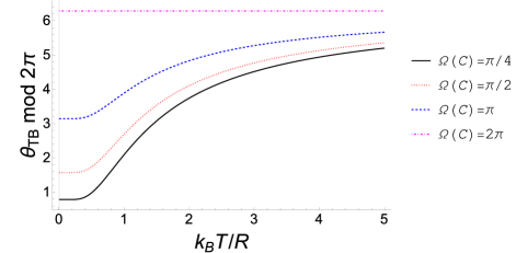
where $\Omega(C)=\oint_{C}\left(1-\cos\theta\right)\mathrm{d}\phi$ is the solid angle enclosed by the loop $C$, and $\lambda_{+}+\lambda_{-}=1$ has been applied in the last step. Therefore, the thermal Berry phase in this case only comes from the contribution of the first term of Eq. (IV.2.1) and indeed carries geometrical information as the system follows a loop $C$ in the Bloch ball. If $\Omega(C)=2\pi$, i.e. $C$ is a great circle on $S^{2}$ such as the meridian or equator, we have $\theta_{TB}=\pm 2\pi=0$ (mod $2\pi$) at any temperature, which is a trivial phase. To visualize the result, we plot $\theta_{TB}$ vs. temperature for different values of $\Omega(C)$ in Fig. 1. At zero temperature, all results reduce to twice the ordinary Berry phase of the double-mode ground state $|R_{-}\rangle\otimes|\tilde{R}_{-}\rangle$. The factor of $2$ comes from the equal contributions of both the system and ancilla. As the infinite-temperature limit is approached, $\theta_{TB}\rightarrow 2\pi(=0$ mod $2\pi)$ for any loop $C$. In this case, the density matrix corresponds to the center of the Bloch ball. Thus, any loop $C$ shrinks to a single point, which has a trivial topology. Hence, the thermal Berry phase is trivial in the infinite-temperature limit. More technical details of this example, including a classification of the equivalence class of mixed states based on the Berry phase, can be found in Appendix B.

In contrast, if a purified state of the system plus ancilla is constructed for the same case, the thermal Berry phase can be shown to be identically zero (mod $2\pi$), as it lacks geometrical information in this case. We remark that the thermal Berry phase counts the contributions from both the system and ancilla. In the case of a purified state, the total contribution vanishes at any temperature. Therefore, this example clearly shows that the thermal Berry phase can be used to distinguish the two different representations of mixed states (except the case with infinite temperature and the case with a great circle in the parameter space). We emphasize the result is quite general: As long as a Hamiltonian leads to a nontrivial thermal Berry phase for a thermal vacuum, the system can distinguish the result from a purified state since the thermal Berry phase is always zero for a purified state.

The thermal Berry phase already predicts interesting results for differentiating a thermal vacuum and purified state. However, the physical role of the thermal Hamiltonian $\hat{H}_{\beta}$ is worth more investigations. Moreover, the thermal Berry phase may contain non-geometrical information. Here we presents another approach towards a geometrical generalization of the Berry phase. Note the system plus ancilla of a purified state is governed by the Hamiltonian $\hat{H}\otimes\tilde{H}$. When compared to the thermal Berry phase, we may instead consider a composite state $|W(t)\rangle$ evolving adiabatically under the composite Hamiltonian $\hat{H}\otimes\tilde{H}$, which has a more physical meaning comparing to the temperature-dependent $\hat{H}_{\beta}$. Moreover, this adiabatic evolution can be incorporated in certain composite unitary transformations that the composite system undergoes, as long as the related parallel-transport condition is satisfied. By replacing $|\psi(t)\rangle$ in Eq. (4) by $|W(t)\rangle$, we obtain the parallel-transport condition in this case:

where $|W(t)\rangle$ is the purified state of $\rho(t)$. The dependence of $\rho$ on $t$ is via a $t$-dependent curve $\mathbf{R}(t)$: $\rho(t)\equiv\rho(\mathbf{R}(t))$. The density matrix here describes the system while its purification includes the ancilla. Using similar derivations, the corresponding parallel-transport conditions can also be constructed for a thermal vacuum. We present analyses of different types of unitary transformations in the following subsections.

References

- Berry [1984] M. V. Berry, Proc. R. Soc. A 392, 45 (1984).
- Simon [1983] B. Simon, Phys. Rev. Lett. 51, 2167 (1983).
- Wilczek and Zee [1984] F. Wilczek and A. Zee, Phys. Rev. Lett. 52, 2111 (1984).
- Bohm et al. [2003] A. Bohm, A. Mostafazadeh, H. Koizumi, Q. Niu, and J. Zwanziger, The geometric phase in quantum systems (Springer, Berlin, Germany, 2003).
- Vanderbilt [2018] D. Vanderbilt, Berry Phases in Electronic Structure Theory: Electric Polarization, Orbital Magnetization and Topological Insulators (Cambridge University Press, Cambridge, UK, 2018).
- Cohen et al. [2019] E. Cohen, H. Larocque, F. Bouchard, F. Nejadsattari, Y. Gefen, and E. Karimi, Nat. Rev. Phys. 1, 437 (2019).
- Hasan and Kane [2010] M. Z. Hasan and C. L. Kane, Rev. Mod. Phys. 82, 3045 (2010).
- Qi and Zhang [2011] X.-L. Qi and S.-C. Zhang, Rev. Mod. Phys. 83, 1057 (2011).
- Chiu et al. [2016] C. K. Chiu, J. C. Y. Teo, A. P. Schnyder, and S. Ryu, Rev. Mod. Phys. 88, 035005 (2016).
- Nakahara [2003] M. Nakahara, Geometry, Topology and Physics (Institute of Physics Publishing, Bristol, UK, 2003).
- Thouless et al. [1982] D. J. Thouless, M. Kohmoto, M. P. Nightingale, and M. den Nijs, Phys. Rev. Lett. 49, 405 (1982).
- Haldane [1988] F. D. M. Haldane, Phys. Rev. Lett. 61, 2015 (1988).
- Moore [2010] J. E. Moore, Nature 464, 194 (2010).
- Kane and Mele [2005a] C. L. Kane and E. J. Mele, Phys. Rev. Lett. 95, 226801 (2005a).
- Kane and Mele [2005b] C. L. Kane and E. J. Mele, Phys. Rev. Lett. 95, 146802 (2005b).
- Bernevig and Zhang [2006] B. A. Bernevig and S.-C. Zhang, Phys. Rev. Lett. 96, 106802 (2006).
- Moore and Balents [2007] J. E. Moore and L. Balents, Phys. Rev. B 75, 121306(R) (2007).
- Fu et al. [2007] L. Fu, C. L. Kane, and E. J. Mele, Phys. Rev. Lett. 98, 106803 (2007).
- Bernevig and Hughes [2013] B. A. Bernevig and T. L. Hughes, Topological Insulators and Topological Superconductors (Princeton, NJ, 2013).
- Uhlmann [1986] A. Uhlmann, Rep. Math. Phys. 24, 229 (1986).
- Uhlmann [1989] A. Uhlmann, Ann. Phys. (Berlin) 501, 63 (1989).
- Uhlmann [1991] A. Uhlmann, Lett. Math. Phys. 21, 229 (1991).
- Uhlmann [1996] A. Uhlmann, J. Geom. Phys. 18, 76 (1996).
- Guo et al. [2020] H. Guo, X.-Y. Hou, Y. He, and C.-C. Chien, Phys. Rev. B 101, 104310 (2020).
- Budich and Diehl [2015a] J. C. Budich and S. Diehl, Phys. Rev. B 91, 165140 (2015a).
- Umezawa et al. [1982] H. Umezawa, H. Matsumoto, and M. Tachiki, Dynamics and Condensed States (North-Holland, 1982).
- Das [1999] A. Das, Finite Temperature Field Theory (World Scientific, 1999).
- Blasone et al. [2011] M. Blasone, P. Jizba, and G. Vitiello, Quantum field theory and its macroscopic manifestations: Boson condensation, ordered patterns and topological defects (Academic Press, Burlington, USA, 2011).
- Cottrell et al. [2019] W. Cottrell, B. Freivogel, D. M. Hofman, and S. F. Lokhande, JHEP 2019, 58 (2019).
- Gao et al. [2017] P. Gao, D. L. Jafferis, and A. C. Wall, J. High Energy Phys. 2017, 151 (2017).
- Susskind and Zhao [2018] L. Susskind and Y. Zhao, Phys. Rev. D 98, 046016 (2018).
- Viyuela et al. [2018] O. Viyuela, A. Rivas, S. Gasparinetti, A. Wallraff, S. Filipp, and M. A. Martin-Delgado, npj Quant. Inf. 4, 10 (2018).
- Zhu et al. [2020] D. Zhu, S. Johri, N. M. Linke, and C. Monroe, Proc. Natl. Acad. Sci. 117, 25402 (2020).
- Alber et al. [2001] G. Alber, T. Beth, M. Horodecki, P. Horodecki, R. Horodecki, M. Rotteler, H. Weinfurter, R. Werner, and A. Zeilinger, Quantum information: An introduction to basic theoretical concepts and experiments (Springer, Berlin, Germany, 2001).
- Lim et al. [2011a] H.-T. Lim, Y.-S. Ra, Y.-S. Kim, J. Bae, and Y.-H. Kim, Phys. Rev. A 83, 020301(R) (2011a).
- Lim et al. [2011b] H.-T. Lim, Y.-S. Kim, Y.-S. Ra, J. Bae, and Y.-H. Kim, Phys. Rev. Lett. 107, 160401 (2011b).
- Lim et al. [2012] H.-T. Lim, Y.-S. Kim, Y.-S. Ra, J. Bae, and Y.-H. Kim, Phys. Rev. A 86, 042334 (2012).
- Sjqvist et al. [2000] E. Sjqvist, A. K. Pati, A. Ekert, J. S. Anandan, M. Ericsson, D. K. L. Oi, and V. Vedral, Phys. Rev. Lett. 85, 2845 (2000).
- Bhandari [2002] R. Bhandari, Phys. Rev. Lett. 89, 268901 (2002).
- Anandan et al. [2002] J. Anandan, E. Sjqvist, A. K. Pati, A. Ekert, M. Ericsson, D. K. L. Oi, and V. Vedral, Phys. Rev. Lett. 89, 268902 (2002).
- Slater [2002] P. B. Slater, Lett. Math. Phys. 60, 123 (2002).
- Singh et al. [2003] K. Singh, D. M. Tong, K. Basu, J. L. Chen, and J. F. Du, Phys. Rev. A 67, 032106 (2003).
- Andersson and Heydari [2013] O. Andersson and H. Heydari, New J. Phys. 15, 053006 (2013).
- Bardyn et al. [2018] C. E. Bardyn, L. Wawer, A. Altland, M. Fleischhauer, and S. Diehl, Phys. Rev. X 8, 011035 (2018).
- Wang [2019] Z. C. Wang, Sci. Rep. 9, 13258 (2019).
- Ericsson et al. [2003] M. Ericsson, E. Sjöqvist, J. Brännlund, D. K. L. Oi, and A. K. Pati, Phys. Rev. A 67, 020101(R) (2003), URL https://link.aps.org/doi/10.1103/PhysRevA.67.020101.
- Carollo et al. [2003] A. Carollo, I. Fuentes-Guridi, M. F. Santos, and V. Vedral, Phys. Rev. Lett. 90, 160402 (2003), URL https://link.aps.org/doi/10.1103/PhysRevLett.90.160402.
- de Faria et al. [2003] J. G. P. de Faria, A. F. R. de Toledo Piza, and M. C. Nemes, EPL 62, 782 (2003), URL https://doi.org/10.1209/epl/i2003-00440-4.
- Tong et al. [2004] D. M. Tong, E. Sjöqvist, L. C. Kwek, and C. H. Oh, Phys. Rev. Lett. 93, 080405 (2004), URL https://link.aps.org/doi/10.1103/PhysRevLett.93.080405.
- Kwek et al. [2006] L. C. Kwek, D. M. Tong, J. L. Chen, J. F. Du, K. W. Choo, R. Ravishankar, D. Kaszlikowski, and C. H. Oh, Laser Phys. 16, 398 (2006).
- Hou et al. [2020] X.-Y. Hou, Q.-C. Gao, H. Guo, Y. He, T. Liu, and C. C. Chien, Phys. Rev. B 102, 104305 (2020).
- Budich and Diehl [2015b] J. C. Budich and S. Diehl, Phys. Rev. B 91, 165140 (2015b).
- Watrous [2018] J. Watrous, The theory of quantum information (Cambridge University Press, Cambridge, 2018).
- Nielsen and Chuang [2000] M. A. Nielsen and I. L. Chuang, Quantum computation and quantum information (Cambridge University Press, Cambridge, UK, 2000).
- Hou et al. [2021] X.-Y. Hou, H. Guo, and C.-C. Chien, Phys. Rev. A 104, 023303 (2021).
- Matsubara [1955] T. Matsubara, Prog. Theo. Phys 14, 351 (1955).
- Abrikosov et al. [1963] A. A. Abrikosov, L. P. Gorkov, and I. E. Dzyaloshinski, Methods of quantum field theory in statistical physics (Dover publications inc., New York, 1963).
- Keldysh [1965] L. V. Keldysh, Soviet Phys. JETP 20, 1018 (1965).
- Kapusta and Gale [2006] J. I. Kapusta and C. Gale, Finite-temperature field theory: Principles and applications (Cambridge University Press, Cambridge, UK, 2006).
- Greenberger et al. [2009] D. Greenberger, K. Hentschel, and F. Weinert, Compendium of Quantum Physics: Concepts, Experiments, History and Philosophy (Springer, 2009).
- Yi et al. [2005] X. X. Yi, H. T. Cui, Y. H. Lin, and H. S. Song, Phys. Rev. A 71, 022107 (2005).
- Peres [1996] A. Peres, Phys. Rev. Lett. 77, 1413 (1996).
- Perelomov [1986] A. Perelomov, Generalized Coherent States and Their Applications (Springer-Verlag, 1986).
- Chruscinski and Jamiolkowski [2004] D. Chruscinski and A. Jamiolkowski, Geometric Phases in Classical and Quantum Mechanics (Birkhauser, 2004).