Generalized Adiabatic Theorems: Quantum Systems Driven by Modulated Time-Varying Fields
Abstract
We present generalized adiabatic theorems for closed and open quantum systems that can be applied to slow modulations of rapidly varying fields, such as oscillatory fields that occur in optical experiments and light induced processes. The generalized adiabatic theorems show that a sufficiently slow modulation conserves the dynamical modes of time dependent reference Hamiltonians. In the limiting case of modulations of static fields, the standard adiabatic theorems are recovered. Applying these results to periodic fields shows that they remain in Floquet states rather than in energy eigenstates. More generally, these adiabatic theorems can be applied to transformations of arbitrary time-dependent fields, by accounting for the rapidly varying part of the field through the dynamical normal modes, and treating the slow modulation adiabatically. As examples, we apply the generalized theorem to (a) predict the dynamics of a two level system driven by a frequency modulated resonant oscillation, a pathological situation beyond the applicability of earlier results, and (b) to show that open quantum systems driven by slowly turned-on incoherent light, such as biomolecules under natural illumination conditions, can only display coherences that survive in the steady state.
I Introduction
Quantum systems driven by slowly varying external fields play an important role in atomic, molecular and optical physics. The ubiquity of these processes has led to sustained interest in powerful adiabatic theorems (AT’s) that characterize their dynamics Born and Fock (1928); Kato (1950); Sarandy and Lidar (2005); Messiah (2017). The best known AT states that a system initialized in an energy eigenstate will remain in that state when driven by a slowly varying field. Adiabatic processes have found far reaching utility in quantum dynamics Landau (1932); Zener (1932) and in the development of Adiabatic Quantum Computing (AQC) where they are used to reliably realize quantum state transformations Albash and Lidar (2018); Barends et al. (2016). Moreover, adiabaticity conditions bound the allowable speed of state transformations, setting the time cost of AQC algorithms and spurring efforts to find shortcuts to adiabaticity Torrontegui et al. (2017); del Campo (2013); Torrontegui et al. (2013); Campo and Boshier (2012). However, ATs fail for oscillating fields Amin (2009); Du et al. (2008); Tong et al. (2005); Marzlin and Sanders (2004), since these fields can induce transitions between energy eigenstates, precisely the opposite of what is required in traditional adiabatic theorems. Hence traditional ATs can not, in general, be applied to light-induced processes in either isolated or open quantum systems.
Adiabatic dynamics have been successfully deployed in experimental settings through Adiabatic Rapid Passage (ARP)Malinovsky and Krause (2001) and Stimulated Raman Adiabatic Passage (STIRAP) Vitanov et al. (2017); Bergmann et al. (2015) techniques. In these experiments, the adiabatic theorem provides a robust mechanism for high fidelity state preparation that is not sensitive to slight perturbations in the system properties and has been used, for example, to study molecular reaction dynamics Kaufmann et al. (2001) and in the preparation of ultra-cold molecules Külz et al. (1996); Aikawa et al. (2010). However, the domain of these techniques has been limited by the applicability of the AT, limiting the forms of driving fields and transformation times that can be realized. By relaxing key restrictions imposed by the traditional AT, the AMT introduced below significantly broadens the range of experimental techniques, unlocking the potential for faster, more flexible state preparation and system dynamics.
Numerous scenarios do not admit traditional adiabatic approaches. Natural light-induced excitation of biological molecules (e.g., in photosynthesis or vision) provides a particularly important example of a challenge to standard ATs insofar as it involves incoherent excitation of open quantum systems with turn-on times that are exceedingly long compared to the time scale of molecular dynamics. For example, human blinking, the turn-on time of light in vision, occurs over 0.2 sec as compared to the timescale of molecular isomerization induced by incident light in vision which can, under pulsed laser excitation, occur in 50 fs or less. Thus, challenging questions related to the creation of molecular coherences in such natural processes requires an AT adapted to oscillating incoherent fields in open quantum systems Dodin and Brumer (2019); Dodin et al. (2016); Cheng and Fleming (2009); Chenu and Scholes (2015).
In this paper we derive generalized AT’s, termed Adiabatic Modulation Theorems (AMTs), for open and closed quantum systems that apply to oscillatory and other rapidly varying fields, extending adiabaticity conditions to optically driven processes and providing faster pathways to adiabaticity, with the potential to accelerate AQC. Moreover, we show that the adiabatic transformation time is limited not by the energy gaps in the systems but rather by the frequency differences of the instantaneous normal modes, that are often easier to manipulate. These results exploit the fact that many complicated fields of interest are time-dependent modulations (e.g., frequency and amplitude modulated oscillations) of simpler fields that have well understood dynamics.
The AMT’s derived below show that a system subjected to a sufficiently slow modulation of a time-dependent field conserves the dynamical modes of time-dependent reference Hamiltonians. These theorems contain traditional ATs in the limit of modulations of static fields, and generalize easily to modulations of periodic fields, which are shown to preserve Floquet states rather than energy eigenstates. Moreover, we show that the adiabatic transformation time is limited not by the energy gaps in the system but rather by the frequency differences of the instantaneous normal modes, that are often easier to manipulate. Remarkably, these constructions allow for the design of experimental techniques that go beyond the preparation of time-independent states and allow for the preparation of specific dynamics using the well developed intuition of adiabatic theory.
The AMT theorems are widely applicable and two significant examples are provided below. In the isolated system example, we show how the theorem allows for control of dynamics on the entire Bloch sphere in a two level qubit system. In applications to open systems, the theorem resolves a longstanding controversy regarding the role of light-induced coherent oscillations in biophysical processes. The generality of the theorems ensure applications to a wide variety of alternative systems.
II The Adiabatic Modulation Theorems
II.1 Isolated Systems
Consider a family of time-dependent reference Hamiltonians indexed by the parameter (e.g. may be an amplitude or frequency ). For each value of , setting , we define the instantaneous normal modes as
| (1) |
where is the dynamical phase, is an instantaneous quasienergy and the is the instantaneous normal mode of .
These normal modes and corresponding quasienergies are found by solving the eigenproblem
| (2) |
where . That is, the normal modes are particular solutions to the Time-Dependent Schrödinger Equation (TDSE),
| (3) |
and are well understood for many driving fields. For example, for time-independent Hamiltonians, the normal modes of static Hamiltonians are energy eigenstates, while for periodic Hamiltonians they are Floquet states.
A modulation of a time-dependent Hamiltonian, , is a transformation that varies over a time interval through a modulation protocol . The resultant modulated field sweeps through the Hamiltonian family defined above (e.g. a field with a time-dependent amplitude for ). Note, as an aside, that this is an operator generalization of modulations in signal processing and encoding theory Byrne (1993). Generally, the modulated Hamiltonian can be significantly more complicated than since the modulation function may be highly nonlinear and the modulation parameter can vary non-trivially with time.
The dynamics induced by can now be expressed in terms of instantaneous normal modes of , Eq. (1), to give
| (4) |
where . The instantaneous state of the system can always be expressed in this form since is always Hermitian and therefore has a basis of eigenstates that can be used to expand with coefficient 111The modified Hamiltonian is defined using a partial time derivative and therefore neglects the implicit time-dependence of ..
This approach mirrors that used to derive traditional ATs, but replacing the eigenstates with normal modes and energies with quasienergies. We therefore proceed through a similar path to derive adiabaticity conditions under which a system initialized in a normal mode of will remain in that normal mode at all times. Mathematically, this occurs when are decoupled in the TDSE, Eq. (3). Substituting Eq. (4) into Eq. (3) we find
| (5) |
where we have used the identity and Eq. (2) to cancel terms proportional to . Projecting onto an , yields equations of motion for the coefficients,
| (6) |
where we have suppressed the and dependence for brevity, and . To obtain Eq. (6), Eq. (2) was differentiated with respect to to obtain .
Equation (6) takes the same form as the original adiabatic theorem with cross-coupling between normal modes scaled by a rapidly oscillating term Sarandy and Lidar (2005). As a result normal modes evolve independently of one another when the following condition is satisfied:
| (7) |
where . Consequently, if changes much more slowly than the difference in dynamical mode frequencies, the slow modulation will not cross couple the normal modes of the modulated Hamiltonian.
Equation (7) has several important features. First, if are -independent, then their normal modes are energy eigenstates and all Hamiltonian time-dependence is contained in the modulation. In this case, the AMT reduces to the traditional AT, simply relabeling the time variable as . The AMT then extends previous AT’s by recognizing them as statements about how time-dependent transformations of Hamiltonian fields impact dynamical modes of the TDSE. These coincide with eigenstates for static Hamiltonians but the same insight can be applied to any field with well-understood dynamics. For example, if are periodic, Eq. (7) states that slow modulations do not couple Floquet states. One key distinction of the AMT is that its speed limits are set by the differences in normal mode frequencies which are often easier to manipulate than energy gaps between eigenstates, allowing for faster adiabatic transformations. A numerical example is discussed in Sect. III.1.1.
II.2 Open Systems
Consider now an adiabatic theorem for open quantum systems. To prove this theorem we take an approach inspired by Ref. Sarandy and Lidar (2005). The dynamics of an open quantum system are governed by the Liouville von-Neumann (LvN) equation
| (8) |
in the time-convolutionless form Breuer and Petruccione (2007); Alicki and Lendi (2007); Blum (2012). The double-ket notation is indicates an operator Liouville space with a trace inner product . By analogy with the isolated system we define modulations by starting with a family of time-dependent Liouvillians and allowing the modulation parameter to vary over time to give . A modified Liouvillian can then be defined by .
The LvN equation appears similar to the TDSE [Eq. (3)], suggesting that we may be able to apply the same analysis, but replacing Hamiltonians with Liouvillians. However, the Liouvillian and it’s corresponding modified operator are completely positive but not necessarily Hermitian Alicki and Lendi (2007) and therefore require more care in defining their normal modes. A given modified Liouvillian, , has an incomplete set of left and right eigenvectors and . Associated with each eigenvector is a Jordan Block comprised of generalized eigenvectors that combine to give an orthonormal basis of Liouville space defined by the generalized eigenproblem
| (9a) | |||
| (9b) |
where ,, , and , where is the zero operator. Dynamically, the LvN Equation does not cross couple the Jordan blocks to one another, but can lead to cross coupling within states of the same Jordan block, thereby defining decoupled dynamical subspace. (For a concise summary of Jordan canonical form in the context of quantum adiabatic theorems, see ref. Sarandy and Lidar (2005).)
Motivated by the isolated systems derivation, we consider the modified Liouvillian and aim to expand the dynamics of the open system in terms of its instantaneous generalized eigenstates. These are given by the (right) generalized equation
| (10) |
The left generalized eigenstates can be similarly defined as the right eigenstates of .
Allowing the modulation parameter to change with time, the instantaneous state of the system can be expanded as a superposition over the generalized eigenstates in the form
| (11) |
where is a complex valued expansion coefficient. Similarly, to Eq. (4), any density operator can be expressed in this form since the generalized eigenbasis that generates Jordan canonical form is complete and orthonormal.
Substituting the trial form of Eq. (11) into the time convolutionless Liouville-von Neumann equation [Eq. (8)] and projecting onto the left generalized eigenstate , gives the following equation of motion for the expansion coefficients:
| (12) |
where we have used the Floquet Equation (10) and the orthonormality condition of generalized eigenstates. By convention, we take .
Differentiating Eq. (10) for some right eigenstate with respect to at fixed and projecting onto left eigenstate with gives
| (13) |
This expression can be simplified by first noting that for orthonormality of the basis eliminates the term on the right hand side of Eq. (13). Equation (9a) can then be used to expand the second term, yielding a recursive expression for the projected change of the normal modes.
| (14) |
where . Iterating recursively through Eq. (14), the change in the normal modes can be related to the change in the modulated Liouvillian by
| (15) |
where , and are the summation indexes over states in the Jordan Block.
Finally, by substituting Eq. (15) into Eq. (12) and considering only the terms that couple non-degenerate Jordan blocks , we obtain an adiabaticity condition for slowly modulated open quantum systems:
| (16) |
This expression is admittedly unwieldy but provides a completely general criteria for open system adiabaticity. A number of simpler but less tight bounds can be obtained for the adiabaticity condition by extending the approach discussed in Sarandy and Lidar (2005) that treated constant Liouvillian. The simplest of these results states that if , e.g., in Eq. (12), then the open quantum system undergoes adiabatic dynamics. Moreover, similarly to the closed system adiabatic theorem, Eq. (16) can be used to derive the earlier non-modulated adiabatic theorem of Ref. Sarandy and Lidar (2005) by assuming a constant .
A significant example of the open system AMT is provided in Sect. III.2 where the theorem is applied to the slowly turned-on incoherent (e.g., solar radiation) excitation of molecular systems.
III Computational Examples
III.1 Isolated Systems
III.1.1 Rabi type system
In this section, we consider a two-level system (TLS) driven by a frequency modulated oscillatory field. We begin by defining an extension of the Rabi model, the family of Hamiltonians,
| (17) |
that characterize driving by a field with frequency . Here is the energy difference between the states and , the coupling coefficient is given by , is the electric field vector driving the system, is the transition dipole moment between the two states and we have set . This family of Hamiltonians comprises the standard Rabi model with well understood dynamics for all values of .
It is useful to briefly review the dynamics induced by Eq. (17) from the perspective of Floquet’s theorem to highlight the normal modes that play an important role in the generalized adiabatic theorem. Since is periodic with period , it’s dynamical normal modes are two -periodic Floquet states, with time-independent quasienergies . These states are eigenstates of the Floquet Hamiltonian, satisfying
| (18a) | |||
| (18b) | |||
| . | |||
For the Hamiltonian in Eq. (17), these Floquet states and quasi energies are given by
| (19a) | |||
| (19b) | |||
| (19c) |
where is the detuning, is the coupling phase, is the mixing angle and is the generalized Rabi frequency.
Consider then driving this system by a frequency modulated field with time varying . The resulting Hamiltonian can be expressed as a modulation of the form discussed above with , that sweeps through Hamiltonians in the family described by Eq. (17). In general, this problem does not admit a closed form solution, but is tractable through direct numerical propagation of the TDSE. However, in the limit where the modulation changes sufficiently slowly the dynamics can be solved using the generalized adiabatic theorem for isolated systems [Eq. (7)].
To define the domain in which this theorem applies consider the modulation derivative,
| (20) |
which characterizes the effect of the modulation on the driving field. Given Eq. (19), we have
| (21) |
required for the generalized adiabatic theorem.
Substituting Eqs. (21) and (20) into Eq. (7) shows that the generalized adiabatic theorem applies when
| (22) |
where we have indicated the parameters that change over time upon frequency modulation using the subscript . Here .
When Eq. (22) is well satisfied, then a system initialized in one of the generalized adiabats will remain in that state at all times. To demonstrate this, we consider a simple linear modulation , where is the constant frequency sweep velocity, and where the field, initially in resonance , is swept linearly to . In Fig. 1, numerically exact dynamics are obtained for a range of sweep velocities through Runge-Kutta integration of the TDSE. These dynamics are then compared to the adiabatic theorem predictions, showing excellent agreement for slow modulations. (We note that the time taken to perform this modulation varies significantly for different sweep velocities, and we have plotted the dynamics in Fig. 1 on a normalized time axis .)
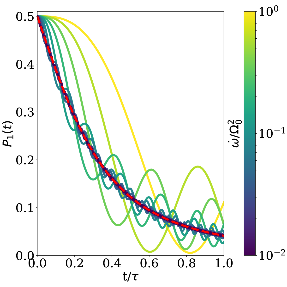
This example is helpful in highlighting the construction and flexibility of the AMT. The adiabatic speed limit is not set by the energy gap but rather by the Rabi frequency on the right hand side of Eq. (22). This feature, typical of the AMT, is remarkable since it allows for manipulation of the adiabatic time scales simply by increasing the intensity of the driving field , and hence , and allows for adiabatic transformations of near degenerate systems on manageable timescales. Moreover, the normal modes, given by the Floquet states , follow the dynamics of the system under fixed frequency driving. By following these oscillatory dynamics the oscillations of the driving field that typically lead to the failure of traditional AT’s are removed from consideration Amin (2009); Du et al. (2008); Tong et al. (2005); Marzlin and Sanders (2004). In this particularly simple case where only one frequency of light drives the system, this is equivalent to moving to a rotating reference frame using the interaction picture. The instantaneous normal modes can therefore be thought of as a more general method for following the dynamics of the system when an interacting reference frame cannot be defined.
III.1.2 Generalizing Adiabatic Experiments
As an indication of the additional role of the AMT in isolated systems, note that it allows a wide range of experimental applications beyond that of the traditional AT. Currently, experimental Adiabatic Rapid Passage (ARP) and Stimulated Raman Adiabatic Passage (STIRAP) techniques have combined the rotating wave approximation with a rotating reference frame in order to apply the traditional AT to optically driven systems. While this approach can be effective for treating systems driven by near-resonant monochromatic lasers or transform limited pulses, it imposes several restrictions on the types of experiments that can be realized. The AMT, however, removes many of these limitations, allowing for driving beyond the Rotating Wave Approximation, driving of a transition by multichromatic fields, and driving of more simultaneous transitions than is allowed under standard conditions. The removal of these limitations can have significant effects on possible experimental techniques. (For example, a recently derived adiabaticity condition Wang and Plenio (2016) allowed for the use of specifically designed pulse sequences to realize adiabatic transformations in finite time. Xu et al. (2019)) Moreover, the AMT allows for the adiabatic treatment of new phenomena that lie far outside of the rotating wave regime, such as Sisyphus cooling, and can address experimental challenges that are intractable using simpler driving protocols, such implementing Stimulated Hyper-Raman Adiabatic Passage in the presence of Autler-Townes shifts from spectator states Guérin et al. (1998); Yatsenko et al. (1998).
To appreciate the advantages afforded by the AMT, consider issues in the application of the traditional AT to oscillatory Hamiltonians. This has been carried out in the Interaction Picture by moving to a rotating reference frame where the oscillatory Hamiltonian time-dependence can be removed. If this can not be done, then the Marzlin-Sanders inconsistency Marzlin and Sanders (2004) prevents application of the traditional adiabatic theorem. Hence, applications of the traditional AT are limited to systems where an appropriate choice of basis and reference Hamiltonian can be found to remove all oscillatory time-dependence.
Consider then the limits of the transformations possible by an appropriate choice of reference Hamiltonian in the Interaction picture. Let be an arbitrary time-dependent Hamiltonian
| (23) |
where are the time-dependent diagonal energies and the off-diagonal couplings.
An interaction picture, such as the commonly used rotating reference frame, is defined by a choice of a reference Hamiltonian . For simplicity, we can work in the eigenbasis of the reference Hamiltonian to give the representation . Equation (23) can then be rewritten in the interaction picture to give
| (24) |
where .
Considering the conditions under which oscillatory time-dependence can be removed from Eq. (24) provides a set of conditions for when AT based approaches can be applied. This requires a basis in which the diagonal elements of have no oscillatory time-dependence, defining the eigenbasis of the reference Hamiltonian . The off diagonal elements show that the only way to eliminate oscillatory time-dependence in is if for a frequency . This condition that prescribes a specific functional form for the time-dependence of is very restrictive and suggests that the strategy of removing oscillatory Hamiltonian time-dependence will only be effective in specific situations. However, this approach has been successful since the oscillatory functional form is precisely what is seen when modelling optically driven transitions in the rotating wave approximation.
This condition, however, does limit the application of the traditional adiabatic theorem to specific types of optical excitation. First, the excitation must be well modelled using the rotating wave approximation. If this is not the case, then the off-diagonal matrix elements would be real valued (e.g. of the form ) and the interaction picture transformation would leave a residual oscillatory component (e.g. of the form ). Moreover, it precludes the driving of one transition by more than one frequency of light, preventing the use of multi-color excitation. Finally, for a discrete dimensional system, the off diagonal elements impose up to conditions conditions on the diagonal elements of . Beyond two-dimensional spin systems, it is not guaranteed that it will be possible to simultaneously satisfy all of these conditions. As a result, removal of oscillatory time-dependence can only be guaranteed when a total of or fewer transitions are driven by an oscillatory external field unless additional resonance conditions are met. The AMT shares none of these limitations.
III.2 Open System Adiabatic Turn-on of Incoherent Light
A particularly important case in open system quantum mechanics involves the adiabatic turn-on of incoherent radiation that is incident on a molecule and the role of quantum coherences in biological processes (e.g photosynthesis and vision). In particular, oscillatory coherences have been observed experimentally in the excitation of biological molecules with pulsed lasers Engel et al. (2007); Zhang et al. (2015); Ishizaki et al. (2010); Johnson et al. (2015). By contrast, we have argued, supported by numerical studies, that natural processes rely upon slowly-turned-on incoherent light, which leads to steady-state transport Jiang and Brumer (1991); Brumer (2018); Dodin and Brumer (2019) with no oscillating coherences. As shown below, the application of the open system adiabatic theorem proves that if a system is driven by very-slowly turned on light, then the only coherences that will be observed are those that survive to the steady state. In particular, the pulsed laser generated coherences noted above do not survive and are irrelevant under natural biological conditions.
Specifically, consider a molecular system initially prepared in the absence of a driving light field. In this case, the system is initially in a simple equilibrium steady state (i.e., with vanishing dynamical frequency). As such, before the radiation field is turned on, the system is found in a Jordan block with zero eigenvalue. At an incoherent light field is turned on on a time scale much slower than the dynamics of the molecule, a typical circumstance in light induced biophysical processes. This corresponds to a modulation in the limit of , ensuring adiabaticity [see Eq. (16] of the underlying dynamics. As a result, at all times, the system is found in a Jordan block with vanishing eigenvalue, that is, in a steady state. This then indicates that the only coherences observed in the slow turn-on limit are those that survive in the steady-state, such as those seen in previous theoretical studies Koyu et al. (2020); Dodin and Brumer (2019); Reppert et al. (2019); Axelrod and Brumer (2018, 2019).
In many cases, consistency with thermodynamics requires the system to have one steady state given by the Gibbs state which shows no coherences between non-degenerate energy eigenstates. This result suggests that the non-steady state coherent dynamics observed under finite turn-on times are a consequence of the rapid turn on of the incoherent light field. Figure 2 discussed below provides a numerical example of these predictions for a popular generic V-system model Dodin and Brumer (2019); Dodin et al. (2016).
The ability to show that no coherent dynamics survive the slow turn-on limit of incoherent light without requiring any calculation highlights the intuitive power of the adiabatic theorems derived in this letter. Notably, this situation is far beyond the bounds of applicability of previous adiabaticity condition as the system dynamics are driven by a noisy incoherent light field. This produces a driving Hamiltonian that fluctuates extremely rapidly, on the order of 1 fs, much faster than the energy gap between states and consequently the underlying molecular dynamics. A numerical example follows below.
Consider then the basic minimal model: an open three level system under irradiation by slowly turned-on incoherent light. This model has been previously treated where numerical results showed Dodin et al. (2016) that coherent dynamics, i.e. coherences in the excited state, vanished under slow turn-on of the exciting field. The system has a ground energy eigenstate, , and two excited states, and that are separated by an energy and is excited by an incoherent light source with time-dependent intensity. The dynamics of this system, in the weak coupling limit, is characterized by the following Partial Secular Bloch-Redfield Master equations for the matrix elements of the density operator :
| (25a) | |||
| (25b) | |||
| (25c) |
where is the spontaneous emission rate and is the rate of excitation to (and stimulated emission from) state . The alignment parameter characterizes the probability of simultaneous excitation to states and and is defined as
| (26) |
where is the transition dipole moment between the ground state and excited state , assumed real for simplicity. The spontaneous emission and excitation rates are related by detailed balance to give where is the mean occupation number of the resonant thermal field mode. It is the slow turn-on of the incoherent light that leads to a time dependent occupation number of the thermal field reflecting it’s time dependent intensity. That is, the slow modulation of the Liouvillian arises due to slow changes in the statistics of the exciting field, in this case in the mean number of photons in the thermal field modes.
These equations of motion can be analytically solved giving several distinct dynamical regimes. In particular, in the limit where , with and , a regime examined below, the system shows long-lived quasi-stationary coherences that eventually decay to give an incoherent thermal state Tscherbul and Brumer (2014). Under excitation by a field with time-dependent intensity of the form , the dynamics are given by
| (27a) | |||
| (27b) |
with and defined above. A detailed derivation of Eq. (27) along with an in depth discussion of the underlying physics are given in Ref. Dodin et al. (2016).
While Eq. (25) is complicated, the dynamics are qualitatively simple. When the turn on time is shorter than the coherence lifetime , the quasi-stationary coherences lead to a potentially long-lived superposition of excited states which rises on a timescale . The coherences then decay on a timescale . As the turn on time becomes comparable to or longer than the coherence lifetime, the quasi-stationary superposition is not fully excited, leading to a decrease in the generated coherences that disappear entirely in the limit. These dynamics are shown for a variety of turn on rates, , in the solid traces of Fig. 2 for the case of , .
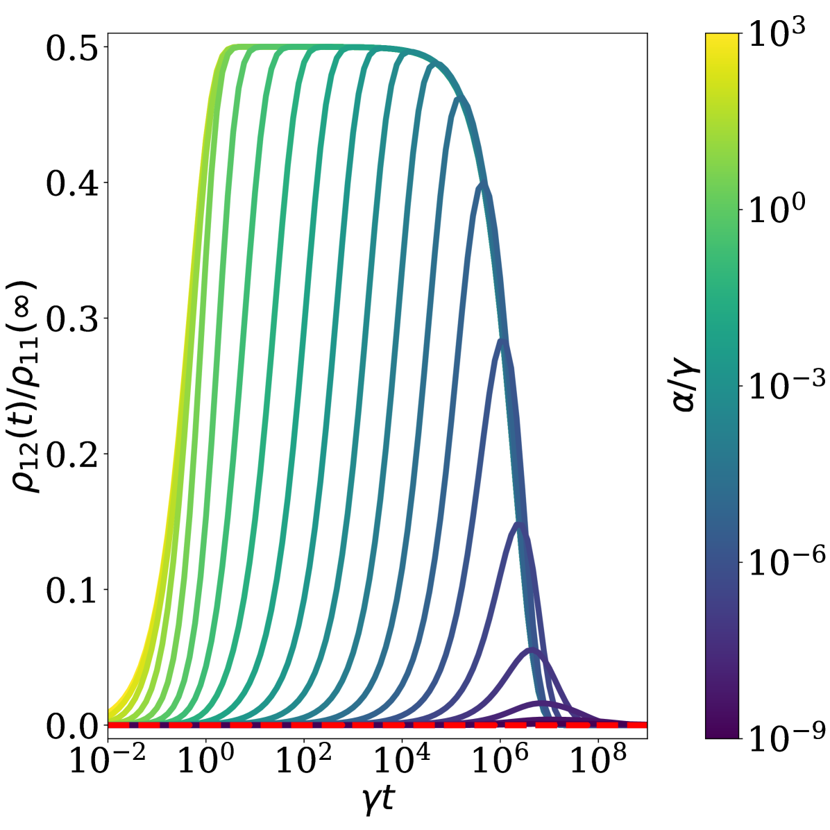
These traces can be compared to the dashed red trace which shows the predictions of the open system adiabatic theorem. As discussed above, since the system is initialized in a steady state of the zero field case, a sufficiently slow turn on leads to dynamics that remain in the instantaneous steady state at . In this example involving only a single bath, the steady state is the thermal Gibbs state with a temperature determined by , and therefore shows no coherences. Consequently, as illustrated in this example, the open systems adiabatic theorem guarantees that a sufficiently slow turn-on of an incoherent field will only show coherences that survive in the steady-state. In the case of two baths, steady state coherences associated with transport will persist Dodin and Brumer (2019); Koyu et al. (2020).
IV Summary
We have presented a new set of generalized adiabatic theorems that apply to rapidly fluctuating fields with slowly varying properties. These results express the dynamics of the modulated field in terms of the dynamical normal modes of time dependent reference Hamiltonians. The resulting adiabaticity conditions take a form that is conceptually similar to preexisting theorems but bounds adiabaticity based on the rate of a slowly changing transformation rather than the rapid underlying field. These results significantly extend the applicability of the adiabatic theorem and its underlying intuition to, e.g., the domain of optical excitations that play a central role in atomic, molecular and optical physics.
Acknowledgments This work was supported by the US Air Force Office of Scientific Research Under Contract Number FA9550-17-1-0310 and FA9550-20-1-0354.
References
- Born and Fock (1928) M. Born and V. Fock, Zeitschrift fur Physik 51, 165 (1928).
- Kato (1950) T. Kato, Journal of the Physical Society of Japan 5, 435 (1950).
- Sarandy and Lidar (2005) M. S. Sarandy and D. A. Lidar, Physical Review A 71, 012331 (2005).
- Messiah (2017) A. Messiah, Quantum Mechanics: Two Volumes Bound As One (Dover Publications, Mineola, N.Y, 2017).
- Landau (1932) L. D. Landau, Phys. Z. Sowjetunion 2, 1 (1932).
- Zener (1932) C. Zener, Proc. R. Soc. Lond. A 137, 696 (1932).
- Albash and Lidar (2018) T. Albash and D. A. Lidar, Reviews of Modern Physics 90, 015002 (2018).
- Barends et al. (2016) R. Barends, A. Shabani, L. Lamata, J. Kelly, A. Mezzacapo, U. L. Heras, R. Babbush, A. G. Fowler, B. Campbell, Y. Chen, Z. Chen, B. Chiaro, A. Dunsworth, E. Jeffrey, E. Lucero, A. Megrant, J. Y. Mutus, M. Neeley, C. Neill, P. J. J. O’Malley, C. Quintana, P. Roushan, D. Sank, A. Vainsencher, J. Wenner, T. C. White, E. Solano, H. Neven, and J. M. Martinis, Nature 534, 222 (2016).
- Torrontegui et al. (2017) E. Torrontegui, I. Lizuain, S. González-Resines, A. Tobalina, A. Ruschhaupt, R. Kosloff, and J. G. Muga, Physical Review A 96, 022133 (2017).
- del Campo (2013) A. del Campo, Physical Review Letters 111, 100502 (2013).
- Torrontegui et al. (2013) E. Torrontegui, S. Ibáñez, S. Martínez-Garaot, M. Modugno, A. del Campo, D. Guéry-Odelin, A. Ruschhaupt, X. Chen, and J. G. Muga, in Advances In Atomic, Molecular, and Optical Physics, Advances in Atomic, Molecular, and Optical Physics, Vol. 62, edited by E. Arimondo, P. R. Berman, and C. C. Lin (Academic Press, 2013) pp. 117–169.
- Campo and Boshier (2012) A. d. Campo and M. G. Boshier, Scientific Reports 2, 648 (2012).
- Amin (2009) M. H. S. Amin, Physical Review Letters 102, 220401 (2009), publisher: American Physical Society.
- Du et al. (2008) J. Du, L. Hu, Y. Wang, J. Wu, M. Zhao, and D. Suter, Physical Review Letters 101, 060403 (2008), publisher: American Physical Society.
- Tong et al. (2005) D. M. Tong, K. Singh, L. C. Kwek, and C. H. Oh, Physical Review Letters 95, 110407 (2005), publisher: American Physical Society.
- Marzlin and Sanders (2004) K.-P. Marzlin and B. C. Sanders, Physical Review Letters 93, 160408 (2004), publisher: American Physical Society.
- Malinovsky and Krause (2001) V. S. Malinovsky and J. L. Krause, European Physical Journal D 14, 147 (2001).
- Vitanov et al. (2017) N. V. Vitanov, A. A. Rangelov, B. W. Shore, and K. Bergmann, Reviews of Modern Physics 89, 015006 (2017), publisher: American Physical Society.
- Bergmann et al. (2015) K. Bergmann, N. V. Vitanov, and B. W. Shore, The Journal of Chemical Physics 142, 170901 (2015), publisher: American Institute of Physics.
- Kaufmann et al. (2001) O. Kaufmann, A. Ekers, C. Gebauer-Rochholz, K. U. Mettendorf, M. Keil, and K. Bergmann, International Journal of Mass Spectrometry Low Energy Electron-Molecule Interactions (Stamatovic honor), 205, 233 (2001).
- Külz et al. (1996) M. Külz, M. Keil, A. Kortyna, B. Schellhaa\S, J. Hauck, K. Bergmann, W. Meyer, and D. Weyh, Physical Review A 53, 3324 (1996), publisher: American Physical Society.
- Aikawa et al. (2010) K. Aikawa, D. Akamatsu, M. Hayashi, K. Oasa, J. Kobayashi, P. Naidon, T. Kishimoto, M. Ueda, and S. Inouye, Physical Review Letters 105, 203001 (2010), publisher: American Physical Society.
- Dodin and Brumer (2019) A. Dodin and P. Brumer, The Journal of Chemical Physics 150, 184304 (2019).
- Dodin et al. (2016) A. Dodin, T. V. Tscherbul, and P. Brumer, The Journal of Chemical Physics 145, 244313 (2016).
- Cheng and Fleming (2009) Y.-C. Cheng and G. R. Fleming, Annual Review of Physical Chemistry 60, 241 (2009).
- Chenu and Scholes (2015) A. Chenu and G. D. Scholes, Annual Review of Physical Chemistry 66, 69 (2015).
- Byrne (1993) C. L. Byrne, Signal Processing: A Mathematical Approach (A K Peters/CRC Press, Wellesley, Mass, 1993).
- Note (1) The modified Hamiltonian is defined using a partial time derivative and therefore neglects the implicit time-dependence of .
- Breuer and Petruccione (2007) H.-P. Breuer and F. Petruccione, The Theory of Open Quantum Systems (Oxford University Press, 2007).
- Alicki and Lendi (2007) R. Alicki and K. Lendi, Lecture Notes in Physics 286 (2007).
- Blum (2012) K. Blum, Density Matrix Theory and Applications (Springer Science & Business Media, 2012).
- Wang and Plenio (2016) Z.-Y. Wang and M. B. Plenio, Physical Review A 93, 052107 (2016), publisher: American Physical Society.
- Xu et al. (2019) K. Xu, T. Xie, F. Shi, Z.-Y. Wang, X. Xu, P. Wang, Y. Wang, M. B. Plenio, and J. Du, Science Advances 5, eaax3800 (2019), publisher: American Association for the Advancement of Science Section: Research Article.
- Guérin et al. (1998) S. Guérin, L. P. Yatsenko, T. Halfmann, B. W. Shore, and K. Bergmann, Physical Review A 58, 4691 (1998), publisher: American Physical Society.
- Yatsenko et al. (1998) L. P. Yatsenko, S. Guérin, T. Halfmann, K. Böhmer, B. W. Shore, and K. Bergmann, Physical Review A 58, 4683 (1998), publisher: American Physical Society.
- Engel et al. (2007) G. S. Engel, T. R. Calhoun, E. L. Read, T.-K. Ahn, T. Mančal, Y.-C. Cheng, R. E. Blankenship, and G. R. Fleming, Nature 446, 782 (2007).
- Zhang et al. (2015) Y. Zhang, S. Oh, F. H. Alharbi, G. S. Engel, and S. Kais, Physical Chemistry Chemical Physics 17, 5743 (2015).
- Ishizaki et al. (2010) A. Ishizaki, T. R. Calhoun, G. S. Schlau-Cohen, and G. R. Fleming, Physical Chemistry Chemical Physics 12, 7319 (2010).
- Johnson et al. (2015) P. J. M. Johnson, A. Halpin, T. Morizumi, V. I. Prokhorenko, O. P. Ernst, and R. J. D. Miller, Nature Chemistry 7, 980 (2015).
- Jiang and Brumer (1991) X.-P. Jiang and P. Brumer, The Journal of Chemical Physics 94, 5833 (1991).
- Brumer (2018) P. Brumer, The Journal of Physical Chemistry Letters 9, 2946 (2018).
- Koyu et al. (2020) S. Koyu, A. Dodin, P. Brumer, and T. V. Tscherbul, arXiv preprint arXiv:2001.09230 (2020).
- Reppert et al. (2019) M. Reppert, D. Reppert, L. A. Pachon, and P. Brumer, arXiv:1911.07606 [quant-ph] (2019), arXiv: 1911.07606.
- Axelrod and Brumer (2018) S. Axelrod and P. Brumer, The Journal of Chemical Physics 149, 114104 (2018), publisher: American Institute of Physics.
- Axelrod and Brumer (2019) S. Axelrod and P. Brumer, The Journal of Chemical Physics OSQD2019, 014104 (2019), publisher: American Institute of Physics.
- Tscherbul and Brumer (2014) T. V. Tscherbul and P. Brumer, Physical Review Letters 113, 113601 (2014).