Generalized Eulerian-Lagrangian description of Navier-Stokes and resistive MHD dynamics

Carlos Cartes Laboratoire de Physique Statistique de l’Ecole Normale Supérieure, associé au CNRS et aux Universités Paris VI et VII, 24 Rue Lhomond, 75231 Paris, France Miguel D. Bustamante Mathematics Institute, University of Warwick, Coventry CV4 7AL, United Kingdom Annick Pouquet National Center for Atmospheric Research, Boulder (CO) 80304 - USA Marc E. Brachet Laboratoire de Physique Statistique de l’Ecole Normale Supérieure, associé au CNRS et aux Universités Paris VI et VII, 24 Rue Lhomond, 75231 Paris, France and National Center for Atmospheric Research, Boulder (CO) 80304 - USA

Abstract

New generalized equations of motion for the Weber-Clebsch potentials that describe both the Navier-Stokes and MHD dynamics are derived. These depend on a new parameter, which has dimensions of time for Navier-Stokes and inverse velocity for MHD. Direct numerical simulations (DNS) are performed. For Navier-Stokes, the generalized formalism captures the intense reconnection of vortices of the Boratav, Pelz and Zabusky flow, in agreement with the previous study by Ohkitani and Constantin. For MHD, the new formalism is used to detect magnetic reconnection in several flows: the $3$ D Arnold, Beltrami and Childress (ABC) flow and the ( $2$ D and $3$ D) Orszag-Tang vortex. It is concluded that periods of intense activity in the magnetic enstrophy are correlated with periods of increasingly frequent resettings. Finally, the positive correlation between the sharpness of the increase in resetting frequency and the spatial localization of the reconnection region is discussed.

pacs:

47.10.-g, 47.11.-j, 47.32.C-, 47.65.-d

I Introduction

The Eulerian-Lagrangian formulation of the (inviscid) Euler dynamics in terms of advected Weber-Clebsch potentials ConstantinLocal was extended by Constantin Constantin to cover the (viscous) Navier-Stokes dynamics. Ohkitani and Constantin (OC) Ohk then performed numerical studies of this formulation of the Navier-Stokes equations. They concluded that the diffusive Lagrangian map becomes noninvertible under time evolution and requires resetting for its calculation. They proposed the observed sharp increase of the frequency of resettings as a new diagnostic of vortex reconnection.

We were able to recently complement these results, using an approach that is based on a generalized set of equations of motion for the Weber-Clebsch potentials that turned out to depend on a parameter $\tau$ which has the unit of time for the Navier-Stokes case CBB07 (the MHD case is different, see below Section II.1.3). The OC formulation is the (singular) $\tau\to 0$ limit case of our generalized formulation. Using direct numerical simulations (DNS) of the viscous Taylor-Green vortex TG1937 we found that for $\tau\neq 0$ the Navier-Stokes dynamics was well reproduced at small enough Reynolds numbers without resetting. However, performing resettings allowed computation at much higher Reynolds number.

The aim of the present article is to extend these results to different flows, both in the Navier-Stokes case and in magnetohydrodynamics, and thereby obtain a new diagnostic for magnetic reconnection. Our main conclusion is that intense reconnection of magnetic field lines is indeed captured in our new generalized formulation as a sharp increase of the frequency of resettings. Here follows a summary of our principal results.

We first derive new generalized equations of motion for the Weber-Clebsch potentials that describe both the Navier-Stokes and MHD dynamics. Performing DNS of the Boratav, Pelz and Zabusky flow Peltz1992 , that was previously used by Ohkitani and Constantin Ohk , we first check that our generalized formalism captures the intense Navier-Stokes vortex reconnection of this flow. We demonstrate the reconnection of vortices is actually occurring at the instant of intense activity in the enstrophy, near the lows of the determinant that trigger the resettings. We then study the correlation of magnetic reconnection with increase of resetting frequency by performing DNS of several prototypical MHD flows: the $3$ D Arnold, Beltrami and Childress (ABC) flow Archontis and the Orszag-Tang vortex in $2$ D OT2D and $3$ D OT3D .

II Theoretical Framework

II.1 General Setting

II.1.1 Weber-Clebsch representation for a class of evolution equations

Let us consider a $3$ D vector field $\mathbf{Z}$ depending on time and ( $3$ -dimensional) space, with coordinates $(x^{1},x^{2},x^{3},t)$ . Assume $\mathbf{Z}$ satisfies an evolution equation of the kind:

	$\displaystyle\frac{D\mathbf{Z}}{Dt}$	$\displaystyle=$	$\displaystyle-\nabla P+\sum_{\alpha=1}^{3}u_{\alpha}\nabla{Z}_{\alpha}+\kappa\triangle\mathbf{Z}\,$		(1)
	$\displaystyle\nabla\cdot\mathbf{Z}$	$\displaystyle=$	$\displaystyle 0\,,$		(2)

where greek indices $\alpha,\beta$ denote vector field components running from $1$ to $3$ , $\mathbf{u}$ is a given $3$ D velocity field and we have used the convective derivative defined by

\frac{D}{Dt}\equiv\frac{\partial}{\partial t}+(\mathbf{u}\cdot\nabla)\,.

In the following sections, two different cases will be considered. In section II.2 (Navier-Stokes case) the vector field $\mathbf{Z}$ will correspond to the velocity field $\mathbf{u}$ , whereas in section II.3 (MHD case) it will correspond to the magnetic vector potential $\mathbf{A}$ .

Let us first recall that performing a change from Lagrangian to Eulerian coordinates on the Weber transformation Lamb leads to a description of the Euler equations as a system of three coupled active vector equations in a form that generalizes the Clebsch variable representation ConstantinLocal .

Our starting point will be to apply this classical Weber-Clebsch representation to the field $\mathbf{Z}$ :

\displaystyle\mathbf{Z}

\displaystyle=

\displaystyle\sum_{i=1}^{3}\lambda^{i}\nabla\mu^{i}-\nabla\phi\,,

(3)

where each element of the $3$ pairs of Weber-Clebsch potentials $(\lambda^{i},\mu^{i}),\,\,i=1,2,3$ is a scalar function.

Performing a variation on the Weber-Clebsch representation (3) yields the relation

\mathbf{\delta Z}=\sum_{i=1}^{3}\left(\delta\lambda^{i}\nabla\mu^{i}-\delta\mu^{i}\nabla\lambda^{i}\right)-\nabla\left(\delta\phi-\sum_{i=1}^{3}\delta\mu^{i}\lambda^{i}\right)\,,

(4)

where the symbol $\delta$ stands for any (spatial or temporal) partial derivative. Taking into account the identity $\left[\nabla,\frac{D}{Dt}\right]\equiv\left(\nabla\mathbf{u}\right)\cdot\nabla$ , it is straightforward to derive from (4) the following explicit expression for the convective derivative of the vector field $\mathbf{Z}$ :

\frac{D\mathbf{Z}}{Dt}=\sum_{i=1}^{3}\left(\frac{D\lambda^{i}}{Dt}\nabla\mu^{i}-\frac{D\mu^{i}}{Dt}\nabla\lambda^{i}\right)-\sum_{\alpha=1}^{3}Z_{\alpha}\nabla u_{\alpha}-\nabla\left(\frac{D\phi}{Dt}-\sum_{i=1}^{3}\frac{D\mu^{i}}{Dt}\lambda^{i}\right)\,,

(5)

II.1.2 Equations of motion for the potentials

Following steps that are similar to those presented in our previous paper CBB07 , we now derive a system of equations of motion for the Weber-Clebsch potentials (3) that is equivalent to the original equation (1). If we use the RHS of equation (1) to replace the LHS of our general identity (5), the resulting relation can be solved for the time derivative of the potentials:

	$\displaystyle\frac{D\lambda^{i}}{Dt}$	$\displaystyle=$	$\displaystyle\kappa\triangle\lambda^{i}+\widetilde{L}^{i}[\lambda,\mu]$		(6)
	$\displaystyle\frac{D\mu^{i}}{Dt}$	$\displaystyle=$	$\displaystyle\kappa\triangle\mu^{i}+\widetilde{M}^{i}[\lambda,\mu]\,.$		(7)

Here $\widetilde{L}^{i},\widetilde{M}^{i}$ obey the linear equation

\sum_{i=1}^{3}\left(\widetilde{L}^{i}\nabla\mu^{i}-\widetilde{M}^{i}\nabla\lambda^{i}\right)=\widetilde{\mathbf{f}}-\nabla\widetilde{G}\,,

(8)

where

\widetilde{\mathbf{f}}=2\kappa\sum_{i=1}^{3}\sum_{\alpha=1}^{3}\partial_{\alpha}\lambda^{i}\partial_{\alpha}\nabla\mu^{i}

(9)

and $\widetilde{G}[\lambda,\mu]$ is an arbitrary scalar related to the non-unique separation of a gradient part in eq.(5):

\frac{D\phi}{Dt}-P=\sum_{i=1}^{3}\lambda^{i}\widetilde{M}^{i}-\widetilde{G}-\mathbf{u}\cdot\mathbf{Z}.

(10)

The “divergence-less gauge” (2) allows one to express $\phi$ in terms of $\lambda^{i}$ and $\mu^{i}$ , as the solution of the linear equation

\triangle\phi=\sum_{i=1}^{3}\nabla\cdot(\lambda^{i}\nabla\mu^{i}).

(11)

Thus there is no need to solve equation (10) for the field $\phi$ , since this equation is identically satisfied when $\phi$ is determined by eq. (11).

Equation (8) above is a system of $3$ linear equations for the $6$ unknowns $\widetilde{L}^{i},\widetilde{M}^{i}$ . When $\kappa=0$ there is a simple solution to (8): $\widetilde{L}^{i}=\widetilde{M}^{i}=\widetilde{G}=0$ . In this case the evolution equations (6) and (7) represent simple advection.

II.1.3 Moore-Penrose solution and minimum norm

The linear system (8) is underdetermined ( $3$ equations for $6$ unknowns). In order to find a solution to the system we need to impose extra conditions. Since $\widetilde{L}^{i},\widetilde{M}^{i}$ appear in the equations on an equal footing, it is natural to supplement the system by a requirement of minimum norm, namely that

\sum_{i=1}^{3}(\widetilde{L}^{i}\widetilde{L}^{i}+{\tau^{-2}}\widetilde{M}^{i}\widetilde{M}^{i})

(12)

be the smallest possible (this is the so-called general Moore-Penrose approach Moore ; Penrose ; Ben-Israel , see also our previous paper CBB07 ). The parameter $\tau$ has physical units equal to $[\widetilde{M}/\widetilde{L}]$ . Using eqs.(6),(7) these are the units of $[\mu/\lambda]$ . It will turn out (see equation (20) below) that $[\mu]=L$ (length) and this implies from eq.(3) that $[\lambda]=[\mathbf{Z}]$ . Therefore the units of $\tau$ are

[\tau]=\frac{L}{[\mathbf{Z}]}.

In the Navier-Stokes case (section II.2) $[\mathbf{Z}]=[\mathbf{u}]=LT^{-1}$ and thus $[\tau]=T$ , whereas in the MHD case (section II.3) $[\mathbf{Z}]=[\mathbf{A}]=L^{2}T^{-1}$ and thus $[\tau]=TL^{-1}$ .

The Moore-Penrose solution to (8), that minimizes the norm (12), is explicitly given in equations (A6,A7) of reference CBB07 . Inserting this solution in (6),(7) we finally obtain the explicit evolution equations

	$\displaystyle\frac{D\lambda^{i}}{Dt}$	$\displaystyle=$	$\displaystyle\kappa\triangle\lambda^{i}+\,\,\,\,\nabla\mu^{i}\cdot\mathbb{H}^{-1}\cdot\left(\widetilde{\mathbf{f}}-\nabla\widetilde{G}\right)$		(13)
	$\displaystyle\frac{D\mu^{i}}{Dt}$	$\displaystyle=$	$\displaystyle\kappa\triangle\mu^{i}-\tau^{2}\,\nabla\lambda^{i}\cdot\mathbb{H}^{-1}\cdot\left(\widetilde{\mathbf{f}}-\nabla\widetilde{G}\right)\,,$		(14)

where $\widetilde{\mathbf{f}}$ is given in eq.(9), the dot product denotes matrix or vector multiplication of $3$ -dimensional tensors, and $\mathbb{H}^{-1}$ is the inverse of the square symmetric $3\times 3$ matrix $\mathbb{H}$ , defined by its components:

\mathbb{H}_{\alpha\beta}\equiv\sum_{i=1}^{3}\left(\tau^{2}\,\partial_{\alpha}\lambda^{i}\partial_{\beta}\lambda^{i}+\partial_{\alpha}\mu^{i}\partial_{\beta}\mu^{i}\right)\,.

(15)

These evolution equations together with the particular choice for the arbitrary function $\widetilde{G}$ (see equation (A11) of reference CBB07 )

\widetilde{G}=\triangle^{-1}\nabla\cdot\widetilde{\mathbf{f}},

(16)

is our new algorithm.

In the Navier-Stokes case, we showed in a previous paper CBB07 that the limit $\tau\to 0$ corresponds to the approach used by Ohkitani and Constantin Ohk . In the general case (Navier-Stokes as well as MHD), we remark that the matrix $\mathbb{H}$ (see equation (15)) can be written (using obvious notation) as $\mathbb{H}=(\nabla{\mbox{\boldmath{$\mu$}}})\cdot(\nabla{\mbox{\boldmath{$\mu$}}})^{\rm T}+\tau^{2}(\nabla{\mbox{\boldmath{$\lambda$}}})\cdot(\nabla{\mbox{\boldmath{$\lambda$}}})^{\rm T}$ , which has a very simple structure in the limit $\tau\to 0$ . Because the condition $\det(\nabla{\mbox{\boldmath{$\mu$}}})=0$ is generically obtained at lower codimension than the condition $\det\mathbb{H}=0$ , the limit $\tau\to 0$ is singular.

II.2 Navier-Stokes equations

The standard incompressible NS equations can be written in the form:

	$\displaystyle\frac{D\mathbf{u}}{Dt}$	$\displaystyle=$	$\displaystyle-\nabla\left(p+\frac{1}{2}\|\mathbf{u}\|^{2}\right)+\sum_{\alpha=1}^{3}u_{\alpha}\nabla u_{\alpha}+\nu\triangle\mathbf{u}$
	$\displaystyle\nabla\cdot\mathbf{u}$	$\displaystyle=$	$\displaystyle 0\,,$

which is indeed of the general form (1), (2) with $\mathbf{Z}=\mathbf{u}$ , $\kappa=\nu$ and $P=p+\frac{1}{2}|\mathbf{u}|^{2}$ .

II.3 MHD equations

The standard incompressible MHD equations for the fluid velocity $\mathbf{u}$ and the induction field $\mathbf{b}$ , expressed in Alfvenic velocity units, can be written in the form:

$\displaystyle\frac{D\mathbf{u}}{Dt}$	$\displaystyle=$	$\displaystyle-\nabla p+\nu\triangle\mathbf{u}+(\nabla\times\mathbf{b})\times\mathbf{b}$	(17)
$\displaystyle\frac{D\mathbf{b}}{Dt}$	$\displaystyle=$	$\displaystyle(\mathbf{b}\cdot\nabla)\mathbf{u}+\eta\triangle\mathbf{b}$	(18)
$\displaystyle\nabla\cdot\mathbf{u}$	$\displaystyle=$	$\displaystyle 0$	(19)
$\displaystyle\nabla\cdot\mathbf{b}$	$\displaystyle=$	$\displaystyle 0\,,$

where $\nu$ and $\eta$ are the viscosity and magnetic resistivity, respectively.

We introduce the vector potential in the Coulomb gauge:

	$\displaystyle\mathbf{b}$	$\displaystyle=$	$\displaystyle\nabla\times\mathbf{A}$
	$\displaystyle\nabla\cdot\mathbf{A}$	$\displaystyle=$	$\displaystyle 0\,.$

Using the identity $\nabla\times(\sum_{\alpha=1}^{3}u_{\alpha}\nabla{A}_{\alpha}-(\mathbf{u}\cdot\nabla)\mathbf{A})=(\mathbf{b}\cdot\nabla)\mathbf{u}-(\mathbf{u}\cdot\nabla)\mathbf{b}-(\nabla\cdot\mathbf{u})\mathbf{b}\,$ and the incompressibility condition (19), eq. (18) can be written as

\displaystyle\frac{D\mathbf{A}}{Dt}

\displaystyle=

\displaystyle-\nabla c+\sum_{\alpha=1}^{3}u_{\alpha}\nabla{A}_{\alpha}+\eta\triangle\mathbf{A},

which is indeed of the general form (1) with $\mathbf{Z}=\mathbf{A}$ , $\kappa=\eta$ and $P=c$ .

III Numerical Results

III.1 Implementation

III.1.1 Initial conditions in pseudo-spectral method

Spatially periodic fields can be generated from the Weber-Clebsch representation (3) by setting

\mu^{i}=x^{i}+\mu^{i}_{\rm p},

(20)

and assuming that $\mu^{i}_{\rm p}$ and the other fields $\lambda^{i}$ and $\phi$ appearing in (3) are periodic. Indeed, any given periodic field $\mathbf{Z}$ can be represented in this way by setting

$\displaystyle\mu^{i}_{\rm p}$	$\displaystyle=$	$\displaystyle 0$	(21)
$\displaystyle\lambda^{i}$	$\displaystyle=$	$\displaystyle Z^{i}$	(22)
$\displaystyle\phi$	$\displaystyle=$	$\displaystyle 0.$	(23)

Note that the time independent non-periodic part of $\mu^{i}$ of the form given in (20) is such that the gradients of $\mu^{i}$ are periodic. It is easy to check that this representation is consistent with the generalized equations of motions (13,14). We chose to use standard Fourier pseudo-spectral methods, both for their precision and for their ease of implementation Got-Ors .

III.1.2 Resettings and reconnection

Following Ohkitani and Constantin Ohk , we now define resettings. Equations (21), (22) and (23) are used not only to initialize the Weber-Clebsch potentials at the start of the calculation but also to reset them to the current value of the field $\mathbf{Z}$ , obtained from (3) and (11), whenever the minimum of the determinant of the matrix (15) falls below a given threshold

\det\mathbb{H}\leq\epsilon^{2}.

It is possible to capture reconnection events using resettings. The rationale for this approach is that reconnection events are associated to localized, intense and increasingly fast activity which will drive the potentials to a (unphysical) singularity in a finite time. One way to detect this singularity is via the alignment of the gradients of the potentials, which leads to the vanishing of $\det\mathbb{H}$ at the point(s) where this intense activity or ‘anomalous diffusion’ is taking place. Now, the time scale of this singularity is much smaller than the time scale of the reconnection process itself Ohk , so when $\det\mathbb{H}$ goes below the given threshold and a resetting of the potentials is performed, the anomalous diffusion starts taking place again, more intensely as we approach the fastest reconnection period, driving the new (reset) potentials to a new finite-time singularity, in a time scale that decreases as we approach this period. Therefore, successive resettings will be more and more frequent near the period of fastest reconnection, and that is what we observe in the numerical simulations. This procedure will be used to capture reconnection events in particular flows in both the Navier-Stokes case ( $\mathbf{Z}=\mathbf{u}$ , Section III.2) and the MHD case ( $\mathbf{Z}=\mathbf{A}$ , Sections III.3.2 and III.3.3).

III.2 Navier-Stokes case: BPZ Flow, resettings and reconnection

Ohkitani and Constantin (OC) Ohk used a flow that initially consists of two orthogonally placed vortex tubes that was previously introduced in Boratav, Pelz and Zabusky (BPZ) Peltz1992 to study in detail vortex reconnection. Our previous numerical study of the generalized Weber-Clebsch description of Navier-Stokes dynamics CBB07 was performed using the Taylor-Green vortex, a flow in which vorticity layers are formed in the early stage, followed by their rolling-up by Kelvin-Helmholtz instability Brachet1 . It can be argued Ohk that cut-and-connect type reconnections are much more pronounced in the BPZ flow than in the Taylor-Green flow. In this section we present comparisons, performed on the BPZ flow, of our $\tau\neq 0$ generalized algorithm with direct Navier-Stokes simulations and with OC original approach. The potentials are integrated with resettings in resolution $128^{3}$ for a Reynolds number of $R=1044$ , which is the one used by BPZ and OC.

The BPZ initial data is explicitly given in Peltz1992 .

III.2.1 Comparison of Weber-Clebsch algorithm with DNS of Navier-Stokes

In order to characterize the precision of the $\tau\neq 0$ Weber-Clebsch algorithm, we now compare the velocity field $\mathbf{Z}={\bf u}$ obtained from (3) and (11), by evolving the Weber-Clebsch potentials using (13)–(16), with the velocity field obtained independently by direct Navier-Stokes evolution from the BPZ initial data.

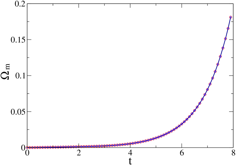
More precisely, we compare the associated kinetic enstrophy $\Omega(t)=\sum_{k}k^{2}E(k,t)$ where the kinetic energy spectrum $E(k,t)$ is defined by averaging the Fourier transform ${\bf\hat{u}}({\bf k^{\prime},t})$ of the velocity field (3) on spherical shells of width $\Delta k=1$ ,

E(k,t)={\frac{1}{2}}\sum_{k-\Delta k/2<|{\bf k^{\prime}}|<k+\Delta k/2}|{\bf\hat{u}}({\bf k^{\prime},t})|^{2}\,.

Refer to caption — Figure 1: Navier-Stokes case: BPZ Flow. Temporal evolution of kinetic enstrophy $\Omega$ for a Reynolds number of $R=1044$ with $\tau=0$ , $0.01$ and $0.1$ ( $+$ , $\circ$ and $\times$ ). The solid line comes from a direct numerical simulation (DNS) at resolution $128^{3}$ .

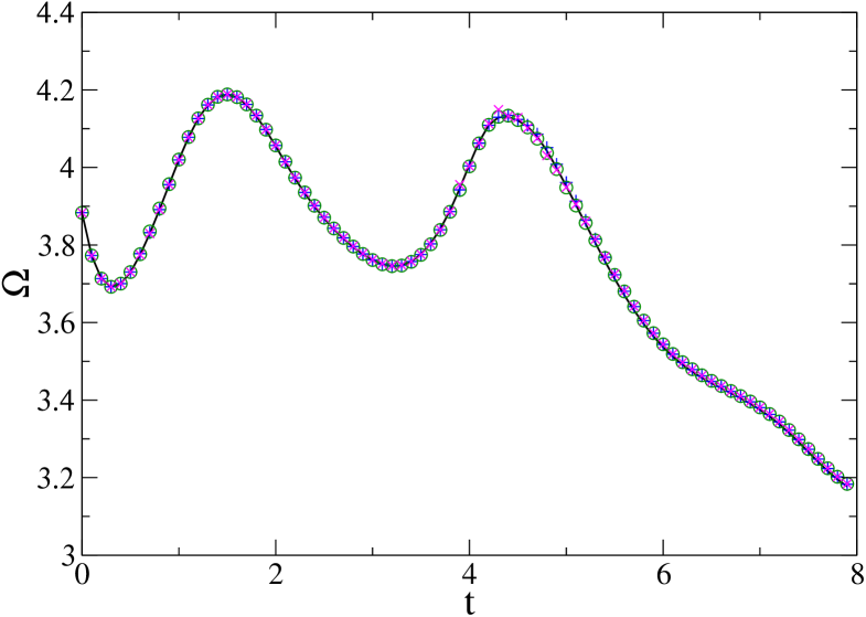
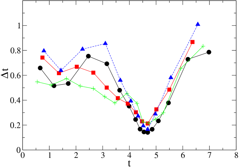
Figure 1 shows that the kinetic enstrophy is well resolved, independently of the choice of the parameter $\tau$ .

III.2.2 Time between resettings as a method for reconnection capture

In this section we study the influence of the parameter $\tau$ on the temporal distribution of the intervals $\Delta t_{j}=t_{j}-t_{j-1}$ between resetting times $t_{j}$ , at fixed value of the resetting threshold $\epsilon^{2}=0.1$ . Using the same Reynolds number and resolution that was used to create Fig. 1, Figure 2 is a plot of $\Delta t$ as a function of time, for simulations with different values of $\tau$ . In the same figure we also show the corresponding $\Delta t$ for a replica of the simulation performed by OC, that is in excellent agreement with our general case.

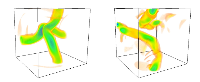
We see that, independently of $\tau$ , there are sharp minima in $\Delta t$ during the periods of maximum enstrophy (see Fig. 1). Inspection of figure 3 demonstrates that the deepest minimum corresponds in fact to the time when reconnection is taking place. The main tubes in the left and right figures are isosurfaces of vorticity corresponding to $60\%$ of the maximum vorticity, which is attained inside each of the main tubes.

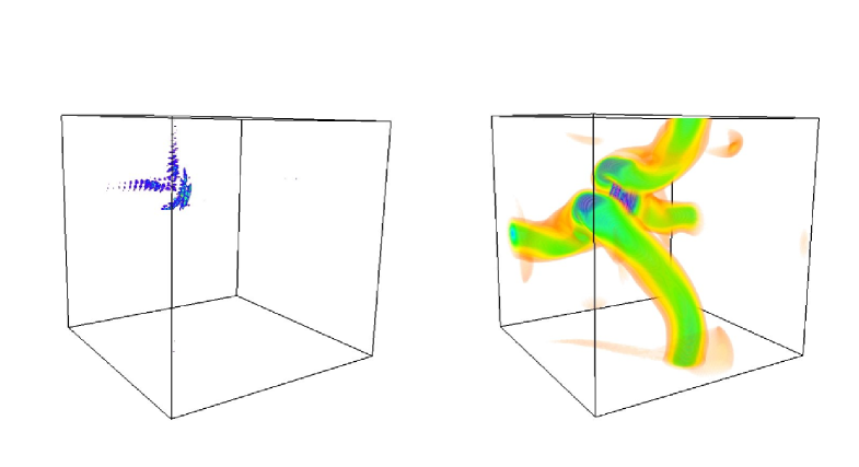
Figure 4 (left) shows that the spatial region where the determinant $\det\mathbb{H}$ goes below the threshold before each resetting corresponds to a small, localized neighborhood between the main interacting vortices. This region is seen in the right figure as a bridge connecting the two vortices: this bridge is an isosurface of vorticity corresponding to $73\%$ of the maximum vorticity, which is attained inside the bridge. The main tubes correspond to isosurfaces of $30\%$ of the maximum vorticity. Note that this behavior of the determinant $\det\mathbb{H}$ is also true for any value of $\tau$ (data not shown), confirming in this way the original rationale for the study of reconnection with the aid of resettings.

Figures 3 and 4 were made using the VAPOR ncarVapor1 ; ncarVapor2 visualization software.

III.3 MHD Flows

In this section we study MHD flows with simple initial conditions. The magnetic potential $\mathbf{Z}=\mathbf{A}$ is obtained in terms of the Weber-Clebsch potentials from (3) and (11), and the Weber-Clebsch potentials are evolved using equations (13)–(16).

We treat the evolution of the velocity field in two different ways: (i) As a kinematic dynamo (ABC flow, Section III.3.1), where the velocity is kept constant in time; (ii) Using the full MHD equations (Orszag-Tang $2$ D and $3$ D, Sections III.3.2 and III.3.3), where the velocity field is evolved using the momentum equation (17).

To compare with DNS of the induction equation (18) for the magnetic field we proceed analogously as in the Navier-Stokes case. We compare the magnetic enstrophy Dahl89 $\Omega_{m}(t)=\sum_{k}k^{2}E_{m}(k,t)$ , where the magnetic energy spectrum $E_{m}(k,t)$ is defined by averaging the Fourier transform ${\bf\hat{b}}({\bf k^{\prime},t})$ of the magnetic field $\mathbf{b}=\nabla\times\mathbf{A}$ (with $\mathbf{A}$ given by (3)) on spherical shells of width $\Delta k=1$ ,

E_{m}(k,t)={\frac{1}{2}}\sum_{k-\Delta k/2<|{\bf k^{\prime}}|<k+\Delta k/2}|{\bf\hat{b}}({\bf k^{\prime},t})|^{2}\,.

Note that magnetic dissipation is the square current.

Resettings will be performed with a resetting threshold $\epsilon^{2}=0.1$ . We have checked that $\epsilon^{2}=0.4$ and $\epsilon^{2}=0.025$ give results that vary only slightly (figures not shown). This is an evidence of the robustness of the resetting method and a validation of the rationale for the use of resettings to diagnose reconnection.

III.3.1 Kinematic dynamo: ABC Flow

We have used the ABC Archontis velocity:

$\displaystyle u_{x}$	$\displaystyle=$	$\displaystyle B_{0}\cos k_{0}y+C_{0}\sin k_{0}z$
$\displaystyle u_{y}$	$\displaystyle=$	$\displaystyle C_{0}\cos k_{0}z+A_{0}\sin k_{0}x$
$\displaystyle u_{z}$	$\displaystyle=$	$\displaystyle A_{0}\cos k_{0}x+B_{0}\sin k_{0}y\,,$

with $k_{0}=2$ and $A_{0}=B_{0}=C_{0}=1$ . We used an initial magnetic seed that reads

$\displaystyle A_{x}$	$\displaystyle=$	$\displaystyle 0$
$\displaystyle A_{y}$	$\displaystyle=$	$\displaystyle 0$
$\displaystyle A_{z}$	$\displaystyle=$	$\displaystyle d_{0}\sin x\sin y\,.$

The magnetic resistivity has been chosen as $\eta=1/12$ and we have set $d_{0}=1/100$ for simplicity (its value is unimportant in the kinematic dynamo).

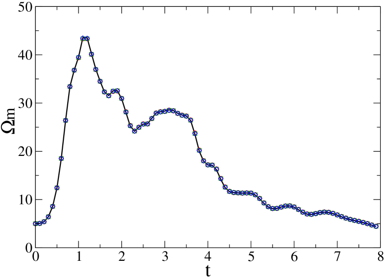
Runs with resettings are compared for different values of the parameter $\tau$ . It is seen in Fig. 5 that the magnetic enstrophy $\Omega_{m}$ is well resolved for each case, at resolution $128^{3}$ .

The resettings are quite regular in time and indeed they slow down as time goes by, at a regular rate which decreases with increasing resolution (figure not shown). There is no increase in the resetting frequency. This behavior is consistent with the monotonic behavior of the magnetic enstrophy and with the absence of localized or intense activity of the magnetic field.

III.3.2 Full MHD equations: 2D Orszag-Tang Vortex

In the rest of the paper, the full MHD equations of motion are integrated. The momentum equation for the velocity (17) is integrated together with the Weber Clebsch evolution equations (13)–(16) where the magnetic potential $\mathbf{Z}=\mathbf{A}$ is obtained from (3) and (11).

We have chosen the following initial data for the $2$ D Orszag-Tang (hereafter, OT) vortex OT2D :

$\displaystyle u_{x}$	$\displaystyle=$	$\displaystyle-2\sin y$
$\displaystyle u_{y}$	$\displaystyle=$	$\displaystyle 2\sin x$
$\displaystyle u_{z}$	$\displaystyle=$	$\displaystyle 0,$
$\displaystyle A_{x}$	$\displaystyle=$	$\displaystyle 0$
$\displaystyle A_{y}$	$\displaystyle=$	$\displaystyle 0$
$\displaystyle A_{z}$	$\displaystyle=$	$\displaystyle 2\cos x\cos 2y\,.$

The OT vortex has a magnetic hyperbolic X-point located at a stagnation point of the velocity, and is a standard test of magnetic reconnection, both in two dimensions add1 and in three dimensions add2 , see below section III.3.3.

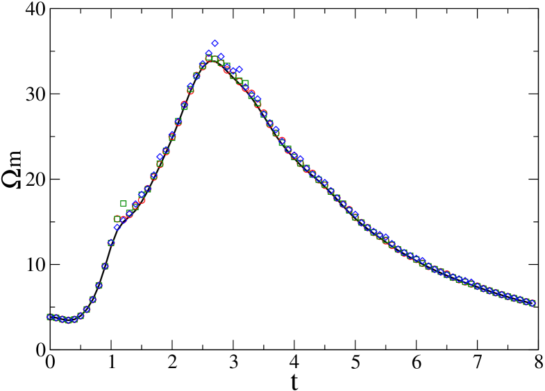
We compare runs with resettings for different values of the parameter $\tau$ . Figure 6 shows that the magnetic enstrophy is well resolved in resolution $128^{2}$ .

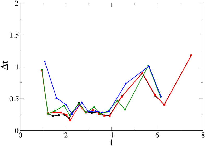
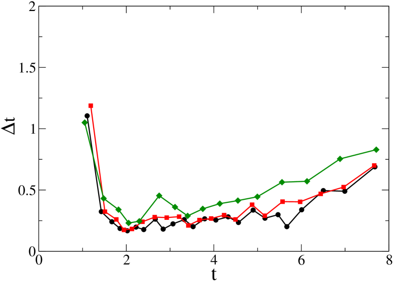
Figure 7 shows the time between resettings as a function of time, for runs performed with different values of $\tau$ . It is apparent from the figure that there are periods of frequent resettings which coincide with the periods of high magnetic enstrophy from Fig. 6. This is a robust evidence of the utility of the resetting approach for $2$ D magnetic reconnection.

We have also simulated the Orszag-Tang vortex in the so-called $2.5$ D setting Montgomery82 (see also the DiPerna-Majda’s construction DiPerna87 ), defined by the same initial data as the above $2$ D Orszag-Tang vortex, but with $A_{x}=\sin y$ and $A_{y}=-\sin x$ . We obtained (data not shown) a behavior of the resetting frequency which was very similar to that of the $2$ D case.

III.3.3 Full MHD equations: 3D Orszag-Tang Vortex

For the $3$ D Orszag-Tang vortex OT3D the initial magnetic potential reads

$\displaystyle A_{x}$	$\displaystyle=$	$\displaystyle c_{0}\left(\cos y-\cos z\right)$
$\displaystyle A_{y}$	$\displaystyle=$	$\displaystyle c_{0}\left(-\cos x+\cos z\right)$
$\displaystyle A_{z}$	$\displaystyle=$	$\displaystyle c_{0}\left(\cos x+\cos 2y\right)\,,$

with $c_{0}=0.8$ . The initial velocity is given by

$\displaystyle u_{x}$	$\displaystyle=$	$\displaystyle-\sin y$
$\displaystyle u_{y}$	$\displaystyle=$	$\displaystyle\sin x$
$\displaystyle u_{z}$	$\displaystyle=$	$\displaystyle 0\,.$

As in the $2$ D case, we compare runs with resettings for different values of the parameter $\tau$ . Figure 8 shows that the magnetic enstrophy is well resolved in resolution $128^{3}$ , and Fig. 9 shows the time between resettings as a function of time. Again the periods of frequent resettings coincide with the periods of high magnetic enstrophy from Fig. 8, proving the utility of the resetting approach for $3$ D magnetic reconnection.

IV Conclusions

We have shown that the generalized Weber-Clebsch evolution equations allow to study reconnection events for both Navier-Stokes and MHD dynamics. We have checked for the Navier-Stokes BPZ flow that reconnection events can be viewed as periods of fast and localized changes in the geometry of the Weber-Clebsch potentials, leading to more and more frequent resetting of the potentials.

We have applied the new generalized Weber-Clebsch evolution equations to the study of magnetic reconnection in MHD. Taking as examples both the $2$ D and $3$ D Orszag-Tang vortices, we show a correlation of the reconnection events (associated to periods of high magnetic dissipation) with the periods of fast changes in the geometry of the Weber-Clebsch potentials, leading to frequent resettings of the potentials.

However, unlike the case of BPZ reconnection, in this case the frequency of resettings does not have a sharp peak but a smeared one. Notice that, in the Navier-Stokes case, the corresponding frequency of resettings for the Taylor-Green vortex has also a mild peak. CBB07 One can argue that the 2D and 3D Orszag-Tang flows are more similar to Taylor-Green than to BPZ. Indeed, both Orszag-Tang and Taylor-Green have initial conditions with just a few Fourier modes, therefore they are extended spatially, whereas the BPZ initial condition is spatially localized (two orthogonal vortex tubes).

This wide spatial extent of the vorticity in both Orszag-Tang and Taylor-Green vortices, as opposed to the localized extent of BPZ, might be the reason for the mildness in the shape of the minimum of the time between resettings. In both spatially extended cases one expects reconnection events to happen in relatively distant places at similar times, as opposed to the BPZ very localized cut-and-connect type of reconnection. In terms of the singularities of the Weber-Clebsch potentials and associated resetting, we should observe (to be studied in detail in future work) that the set of points where $\det\mathbb{H}$ goes below the threshold consists of an extended region, as opposed to BPZ where we have confirmed that these points belong to a very localized region in space. Consequently, the widely distributed events that lead to resetting in Orszag-Tang and Taylor-Green configurations would tend to be less correlated in time, leading to the smearing of the minimum of the curve for the time between resettings, which would otherwise be very sharp if the events were more localized and therefore more correlated in time.

Acknowledgments: We acknowledge very useful scientific discussions with Peter Constantin and Edriss S. Titi. One of the authors (MEB.) acknowledges support from an ECOS/CONICYT action. The computations were carried out at the Institut du Développement et des Ressources en Informatique Scientifique (IDRIS) of the Centre National pour la Recherche Scientifique (CNRS).

References

[1] P. Constantin. An Eulerian–Lagrangian approach for incompressible fluids: Local theory. J. Amer. Math. Soc., 14:263–278, 2001.
[2] P. Constantin. An Eulerian–Lagrangian approach to the Navier–Stokes equations. Commun. Math. Phys., 216:663–686, 2001.
[3] K. Ohkitani and P. Constantin. Numerical study of the Eulerian–Lagrangian formulation of the Navier–Stokes equations. Physics of Fluids, 15(10):3251–3254, 2003.
[4] C. Cartes, M. D. Bustamante, and M. Brachet. Generalized Eulerian-Lagrangian description of Navier-Stokes dynamics. Physics of Fluids, 19:077101, 2007.
[5] G. I. Taylor and A. E. Green. Mechanism of the production of small eddies from large ones. Proc. Roy. Soc. Lond. A, 158:499–521, 1937.
[6] O. N. Boratav, R. B. Pelz, and N. J. Zabusky. Reconnection in orthogonally interacting vortex tubes - direct numerical simulations and quantifications. Physics of Fluids, 4:581–605, March 1992.
[7] V. Archontis, S.B.F. Dorch, and Å. Nordlund. Numerical simulations of kinematic dynamo action. Astronomy & Astrophysics, 397(2):393–399, 2003.
[8] S. A. Orszag and C. M. Tang. Small-scale structure of two-dimensional magnetohydrodynamic turbulence. J. Fluid Mech., 90:129, 1979.
[9] P. D. Mininni, A. G. Pouquet, and D. C. Montgomery. Small-scale structures in three-dimensional magnetohydrodynamic turbulence. Phys. Rev. Lett., 97:244503, 2006.
[10] Lamb H. Hydrodynamics. Cambridge University Press, Cambridge, 1932.
[11] E. H. Moore. On the reciprocal of the general algebraic matrix. Bulletin of the American Mathematical Society, 26:394–395, 1920.
[12] R. Penrose. A generalized inverse for matrices. Proceedings of the Cambridge Philosophical Society, 51:406–413, 1955.
[13] A. Ben-Israel and T. N. E. Greville. Generalized Inverses: Theory and Applications. Wiley-Interscience [John Wiley & Sons], New York, 1974. (reprinted by Robert E. Krieger Publishing Co. Inc., Huntington, NY, 1980.).
[14] D. Gottlieb and S. A. Orszag. Numerical Analysis of Spectral Methods. SIAM, Philadelphia, 1977.
[15] M. E. Brachet, D. I. Meiron, S. A. Orszag, B. G. Nickel, R. H. Morf, and U. Frisch. Small–scale structure of the Taylor–Green vortex. J. Fluid Mech., 130:411–452, 1983.
[16] J. Clyne, P. Mininni, A. Norton, and M. Rast. Interactive desktop analysis of high resolution simulations: application to turbulent plume dynamics and current sheet formation. New Journal of Physics, 9:301, August 2007.
[17] J. Clyne and M. Rast. A prototype discovery environment for analyzing and visualizing terascale turbulent fluid flow simulations. Proceedings of Visualization and Data Analysis, pages 284–294, 2005.
[18] R. B. Dahlburg and J. M. Picone. Evolution of the Orszag-Tang vortex system in a compressible medium. I - Initial average subsonic flow. Physics of Fluids B, 1:2153–2171, November 1989.
[19] H. Politano, A. Pouquet, and P. L. Sulem. Inertial ranges and resistive instabilities in two-dimensional magnetohydrodynamic turbulence. Physics of Fluids B: Plasma Physics, 1(12):2330–2339, 1989.
[20] H. Politano, A. Pouquet, and P. L. Sulem. Current and vorticity dynamics in three-dimensional magnetohydrodynamic turbulence. Physics of Plasmas, 2(8):2931–2939, 1995.
[21] David Montgomery and Leaf Turner. Two-and-a-half-dimensional magnetohydrodynamic turbulence. Physics of Fluids, 25(2):345–349, 1982.
[22] Ronald J. DiPerna and Andrew J. Majda. Oscillations and concentrations in weak solutions of the incompressible fluid equations. Commun. Math. Phys., 108(4):667–689, 1987.