Generalized Gibbons-Werner method for stationary spacetimes

Let $D$ be a compact and connected region on a two-dimensional Riemannian manifold (as depicted in Fig. 1).

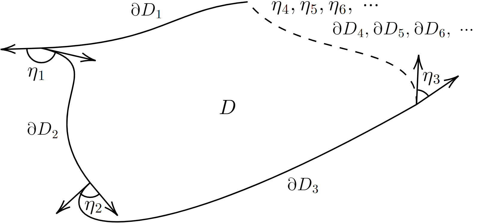
The boundary of $D$, denoted as $\partial D$, consists of piecewise smooth components $\partial D_{i}$ ($i=1,2,\cdots$), and the jump angles at each vertex are represented by $\eta_{i}$ in the positive sense. Then the GBT can be expressed as [73]

$$\iint_{D}K\mathrm{d}S+\sum_{i}\int_{\partial D_{i}}\kappa\mathrm{d}l+\sum_{i}\eta_{i}=2\pi\chi(D),$$

(2.1)

where $K$ and $\mathrm{d}S$ are the Gaussian curvature and area element of $D$, respectively; $\kappa$ and $\mathrm{d}l$ represent the geodesic curvature and line element of $\partial D$, respectively; $\chi(D)$ denotes the Euler characteristic number of $D$.

Eq. (2.1) establishes a fundamental relation between the integral of curvature quantities and the Euler characteristic of the region $D$. The GBT serves as a powerful tool for analyzing the geometric property of surfaces and their topological characteristics.

The JMRF metric, constructed by Chanda $et\ al.$ in 2019 [74], is of great significance in geometrodynamics and provides a framework for studying the particle’s motion in stationary spacetimes. Consider a coordinate $(t,\boldsymbol{x})$ where $\left(\partial/\partial t\right)^{a}$ is the Killing vector corresponding to the stationary property of the spacetime, the metric of the stationary spacetime states

$$\mathrm{d}s^{2}=g_{00}(\boldsymbol{x})\mathrm{d}t^{2}+2g_{0i}(\boldsymbol{x})\mathrm{d}t\mathrm{d}x^{i}+g_{ij}(\boldsymbol{x})\mathrm{d}x^{i}\mathrm{d}x^{j}.$$

(2.2)

Then the corresponding JMRF metric reads [74]

$$\mathrm{d}\tilde{s}=\sqrt{\alpha_{ij}\mathrm{d}x^{i}\mathrm{d}x^{j}}+\beta_{i}\mathrm{d}x^{i},$$

(2.3)

where the components of the JMRF metric are given by

	$\displaystyle\alpha_{ij}$	$\displaystyle=\frac{E^{2}+m^{2}g_{00}}{-g_{00}}\left(g_{ij}-\frac{g_{0i}g_{0j}}{g_{00}}\right),$		(2.4)
	$\displaystyle\beta_{i}$	$\displaystyle=-E\frac{g_{0i}}{g_{00}}.$		(2.5)

Here, $m$ and $E$ stand for the rest mass and relativistic energy of the particle, respectively, and we dropped ’$(\boldsymbol{x})$’ from ’$g_{00}(\boldsymbol{x})$’, ’$g_{0i}(\boldsymbol{x})$’, and ’$g_{ij}(\boldsymbol{x})$’ . The Riemannian metric $\alpha_{ij}$ and one-form $\beta_{i}$ must satisfy the inequality $\sqrt{\alpha^{ij}\beta_{i}\beta_{j}}<1$. We denote the three-dimensional space determined by $\alpha_{ij}$, i.e. the Riemannian part of the JMRF metric, as $M^{\left(\alpha 3\right)}$. For a geodesic in the four-dimensional stationary spacetime Eq. (2.2), its spatial projection $\gamma$ is a geodesic in the three-dimensional JMRF space Eq. (2.3) [74]. Additionally, the JMRF metric encompasses various special cases, including the Jacobi metric applicable to massive particles in SSS spacetimes [75], the optical Randers-Finsler metric applicable to photons in SAS spacetimes [49], and the optical metric applicable to photons in SSS spacetimes [48]. Researchers have utilized the JMRF metric, as well as its specific forms, to investigate the gravitational deflection of particles [48, 49, 76, 77, 50, 78, 75, 79, 80, 51, 81, 82, 83, 58, 52, 53, 84, 85, 63, 86, 54, 87, 88, 89], the Kepler orbit [90], the motion of charged particles [91], and Hawking radiation [92, 93]. A comprehensive discussion on the JMRF metric can be found in [94].

For SAS spacetimes, the metric in the Boyer-Lindquist coordinates can be expressed as

$$\mathrm{d}s^{2}=g_{tt}\left(r,\theta\right)\mathrm{d}t^{2}+g_{rr}\left(r,\theta\right)\mathrm{d}r^{2}+g_{\theta\theta}\left(r,\theta\right)\mathrm{d}\theta^{2}+g_{\phi\phi}\left(r,\theta\right)\mathrm{d}\phi^{2}+2g_{t\phi}\left(r,\theta\right)\mathrm{d}t\mathrm{d}\phi,$$

(2.6)

and the metric of the corresponding $M^{\left(\alpha 3\right)}$ can be written as

$$\mathrm{d}{\hat{l}}^{2}=\alpha_{rr}\left(r,\theta\right)\mathrm{d}r^{2}+\alpha_{\theta\theta}\left(r,\theta\right)\mathrm{d}\theta^{2}+\alpha_{\phi\phi}\left(r,\theta\right)\mathrm{d}\phi^{2}.$$

(2.7)

We focus on the motion in the equatorial plane ($\theta=\pi/2$), and $M^{\left(\alpha 3\right)}$ reduces to a two-dimensional Riemannian space (denoted as $M^{\left(\alpha 2\right)}$ for simplicity). The metric of $M^{\left(\alpha 2\right)}$ reads

$$\mathrm{d}l^{2}=\alpha_{rr}\left(r\right)\mathrm{d}r^{2}+\alpha_{\phi\phi}\left(r\right)\mathrm{d}\phi^{2},$$

(2.8)

in which

$$\alpha_{rr}\left(r\right)=\frac{E^{2}+m^{2}g_{tt}}{-g_{tt}}g_{rr},\qquad\alpha_{\phi\phi}\left(r\right)=\frac{E^{2}+m^{2}g_{tt}}{-g_{tt}}g_{\phi\phi}.$$

(2.9)

The corresponding $\beta_{i}$ states

$$\beta_{\phi}\left(r\right)=-E\frac{g_{t\phi}}{g_{tt}}.$$

(2.10)

Here, we dropped ’$\left(r,\theta=\pi/2\right)$’ from ’$g_{tt}\left(r,\theta=\pi/2\right)$’, ’$g_{rr}\left(r,\theta=\pi/2\right)$’, ’$g_{\phi\phi}\left(r,\theta=\pi/2\right)$’, and ’$g_{t\phi}\left(r,\theta=\pi/2\right)$’ for simplicity.

Furthermore, the equation of motion for unbound particles moving in the equatorial plane of the SAS spacetime equipped with metric (2.6) can be written as [67]

$$\left(\frac{\mathrm{d}u}{\mathrm{d}\phi}\right)^{2}=\frac{u^{4}\left(g_{t\phi}^{2}-g_{tt}g_{\phi\phi}\right)\left[g_{tt}b^{2}v^{2}+2g_{t\phi}bv+g_{\phi\phi}\left(1+g_{tt}-g_{tt}v^{2}\right)+g_{t\phi}^{2}\left(v^{2}-1\right)\right]}{g_{rr}(g_{tt}bv+g_{t\phi})^{2}},$$

(2.11)

where $u=1/r$, $b$ symbolizes the impact parameter, $v$ is the velocity of particles.

In 2017, by taking into account the finite distance from a lens object to a light source and a observer, Ishihara $et\ al.$ investigate the finite-distance corrections for the deflection angle of photons [50]. With the GW method, they defined a finite-distance deflection angle and prove it is geometric invariant, namely well-defined.

As shown in Fig. 2,

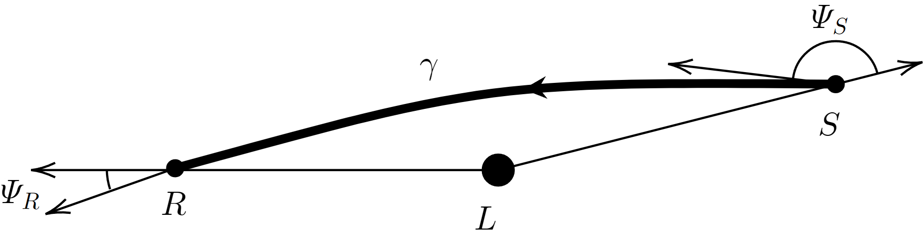
in a two-dimensional Riemannian manifold, $L$ represents the lens, $S$ and $R$ are the source and the receiver of particles, respectively, $\gamma=\overset{\curvearrowright}{SR}$ is the trajectory from $S$ to $R$, then the deflection angle is defined by [50]

$$\delta=\Psi_{R}-\Psi_{S}+\phi_{RS},$$

(2.12)

in which $\phi_{RS}=\phi_{R}-\phi_{S}$ is the increment of the azimuthal coordinate, $\Psi_{S}$ and $\Psi_{R}$ are the angle between the tangent vector along $\gamma$ and the radial outward vector at $S$ and $R$, respectively. In the limit as $S$ and $R$ tend to infinity, $\Psi_{S}=\pi$ and $\Psi_{R}=0$, the above formula reduces to the usual infinite-distance deflection angle $\delta=\phi_{RS}-\pi$. The definition Eq. (2.12) has been widely employed in the investigation of the deflection of particles [80, 51, 55, 59, 58, 61, 95, 60, 63, 54, 96, 87, 64, 97, 98, 65, 66, 99].

As shown in Fig. 3,

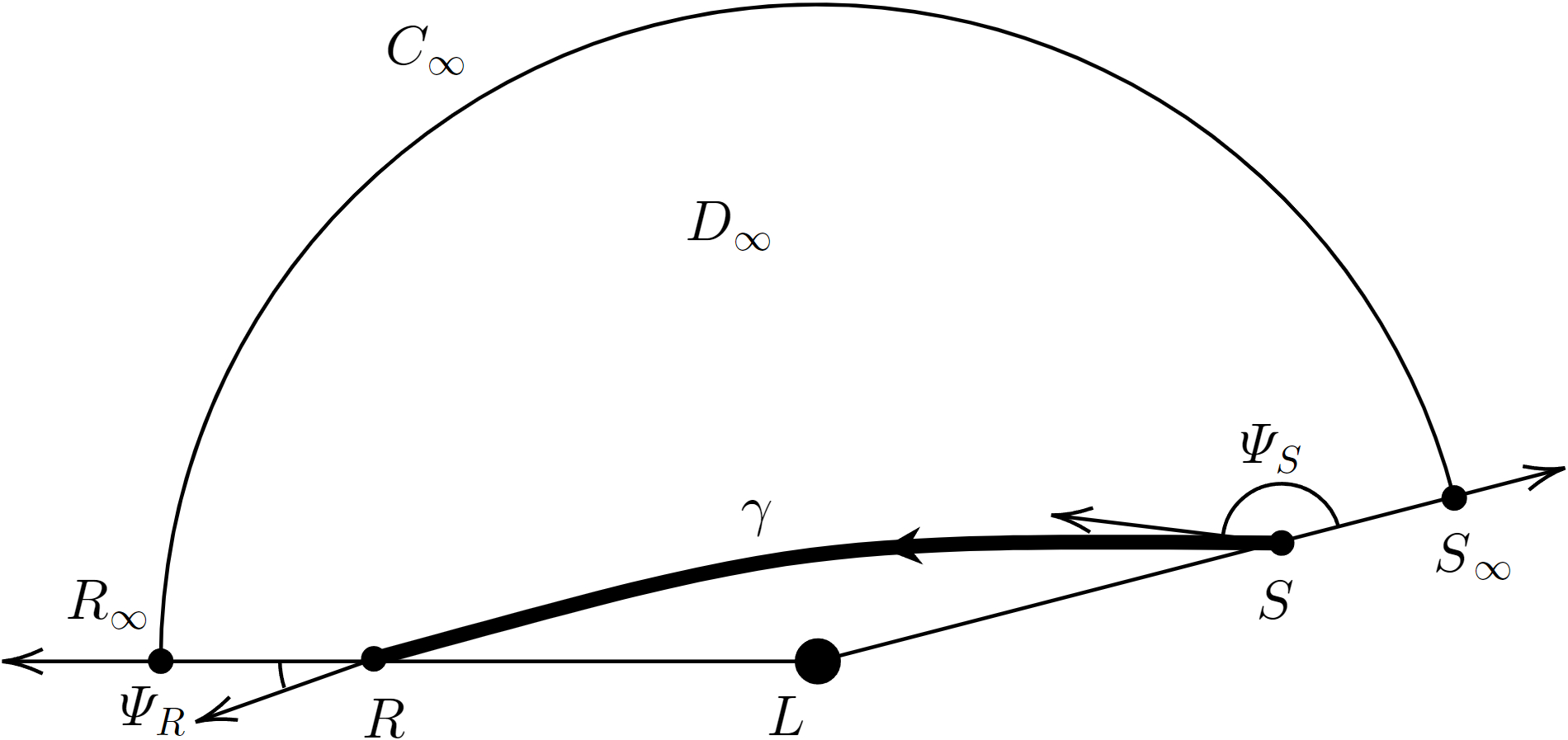
in the $M^{\left(\alpha 2\right)}$ corresponding to the SAS spacetime equipped with metric (2.6), $L$, $S$, $R$, $\gamma$, $\Psi_{S}$, and $\Psi_{R}$ have the same meaning as that in Fig. 2, $C_{\infty}$ is an infinite circular arc, intersecting the outgoing radial curve $\overrightarrow{LS}$ and $\overrightarrow{LR}$ at $S_{\infty}$ and $R_{\infty}$, respectively. Then the integral region is constructed as $D_{\infty}=_{R}^{R_{\infty}}\square_{S}^{S_{\infty}}$. Applying the GBT Eq. (2.1) to $D_{\infty}$ leads to

$$\iint_{D_{\infty}}K\mathrm{d}S+\int_{\overrightarrow{SS}_{\infty}}\kappa\mathrm{d}l+\int_{C_{\infty}}\kappa\mathrm{d}l+\int_{\overrightarrow{R_{\infty}R}}\kappa\mathrm{d}l+\int_{\overset{\curvearrowright}{RS}}\kappa\mathrm{d}l+\eta_{S}+\eta_{S_{\infty}}+\eta_{R_{\infty}}+\eta_{R}=2\pi\chi\left(D_{\infty}\right).$$

(3.3)

$\int_{\overrightarrow{SS}_{\infty}}\kappa\mathrm{d}l=\int_{\overrightarrow{R_{\infty}R}}\kappa\mathrm{d}l=0$, since $\overrightarrow{SS_{\infty}}$ and $\overrightarrow{R_{\infty}R}$ are geodesics (see Appendix A of Ref. [67] for the proof). $\int_{\overset{\curvearrowright}{RS}}\kappa\mathrm{d}l=-\int_{\gamma}\kappa\mathrm{d}l$, $\eta_{S}=\pi-\Psi_{S}$, $\eta_{R}=\Psi_{R}$, $\eta_{S_{\infty}}=\eta_{R_{\infty}}=\pi/2$, and $\chi\left(D_{\infty}\right)=1$ as $D_{\infty}$ is simply connected.

In the scenario where the spacetime is asymptotically flat, $C_{\infty}$ can be treated as a circular arc in the flat space, i.e. $\int_{C_{\infty}}\kappa\cdot\mathrm{d}l=\int_{\phi_{S}}^{\phi_{R}}\left(1/r_{\infty}\right)\cdot r_{\infty}\mathrm{d}\phi=\phi_{RS}$. According to Eq. (3.3) and the related results, we can express the deflection angle as

$$\delta=-\iint_{D_{\infty}}K\mathrm{d}S+\int_{\gamma}\kappa\mathrm{d}l,$$

(3.4)

in which the definition Eq. (2.12) is adopted. The above formula has been used to calculate the deflection angle of particles in Refs. [55, 56, 57, 58, 59, 60, 61, 62, 54, 64, 65, 66, 68], where the spacetime is asymptotically flat.

Based on the presence or absence of the singularity as the radial coordinate approaches infinity, asymptotically nonflat SAS spacetimes can be divided into two categories: the infinity-reachable and the infinity-unreachable. Examples of the infinity-reachable include the Kerr-like black hole in bumblebee gravity [100, 101], while the Kerr-de Sitter spacetime [69] and the rotating solution in conformal Weyl gravity [70, 71] fall under the category of the infinity-unreachable.

In the case of infinity-reachable asymptotically nonflat SAS spacetimes, the construction of an infinite integral region is still allowed. However, the calculation formula of the deflection angle becomes more intricate and relies on the specific metric. To illustrate this, we briefly review the work in [63], where the Kerr-like black hole in bumblebee gravity is considered. The metric for such black hole is given by

$$\mathrm{d}s^{2}=-\left(1-\frac{2Mr}{\rho^{2}}\right)\mathrm{d}t^{2}-\frac{4Mar\lambda\sin^{2}\theta}{\rho^{2}}\mathrm{d}\phi\mathrm{d}t+\frac{\rho^{2}}{\Delta}\mathrm{d}r^{2}+\rho^{2}\mathrm{d}\theta^{2}+\frac{A\sin^{2}\theta}{\rho^{2}}\mathrm{d}\phi^{2},$$

(3.5)

in which $\lambda=\sqrt{1+l}$, $\rho^{2}=r^{2}+\lambda^{2}a^{2}\cos^{2}\theta$, $\Delta=\left(r^{2}-2Mr\right)/\lambda^{2}+a^{2}$, $A=\left(r^{2}+\lambda^{2}a^{2}\right)^{2}-\Delta\lambda^{4}a^{2}\sin^{2}\theta$. Here, $M$ and $a$ are the mass and rotation parameter of the black hole, respectively, and $l$ is the Lorentz violation parameter. In this scenario, Fig. 3 can still serve as the illustration, and the relevant constructions and results, including Eq. (3.3), remain valid except for the integral of the geodesic curvature along $C_{\infty}$. The author derived $\int_{C_{\infty}}\kappa\mathrm{d}l=\left(1/\lambda\right)\phi_{RS}$ instead of the result obtained in asymptotically flat spacetime. Consequently, the deflection angle is expressed as

$$\delta=-\iint_{D_{\infty}}K\mathrm{d}S+\int_{\gamma}\kappa\mathrm{d}l+\left(1-\frac{1}{\lambda}\right)\phi_{RS},$$

(3.6)

in which an additional item, the change in the coordinate angle, appears compared to Eq. (3.4) due to the existence of the bumblebee vector field. It is important to note that the formula for the deflection angle will vary depending on the specific metrics employed.

As for the infinity-unreachable asymptotically nonflat SAS spacetime, the infinite integral region $D_{\infty}$ is ill-defined, rendering the GWOIA method invalid.

As shown in Fig. 4,

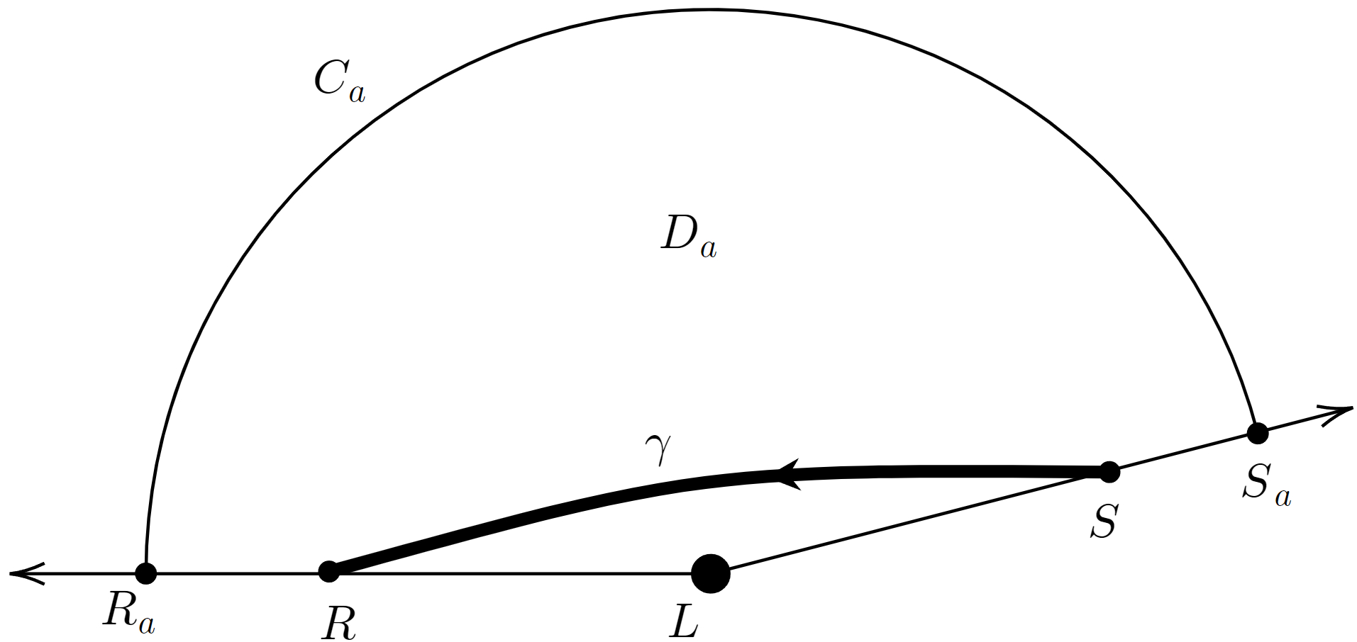
in the $M^{\left(\alpha 2\right)}$, $L$, $S$, $R$, and $\gamma$ have the same meaning as that in Fig. 2. $C_{a}=\overset{\curvearrowright}{S_{a}R_{a}}$ is the auxiliary circular arc with $r_{c}>r_{\gamma}^{max}$, and intersects with $\overrightarrow{LS}$ and $\overrightarrow{LR}$ at $S_{a}$ and $R_{a}$, respectively. Thus we obtain a quadrilateral region $D_{a}=^{R_{a}}_{R}\square^{S_{a}}_{S}$. Here, the subscript $a$ indicates "arbitrary". The application of the GBT to $D_{a}$ yields

$$\iint_{D_{a}}K\mathrm{d}S+\int_{\overrightarrow{SS}_{a}}\kappa\mathrm{d}l+\int_{C_{a}}\kappa\mathrm{d}l+\int_{\overrightarrow{R_{a}R}}\kappa\mathrm{d}l+\int_{\overset{\curvearrowright}{RS}}\kappa\mathrm{d}l+\eta_{S}+\eta_{S_{a}}+\eta_{R_{a}}+\eta_{R}=2\pi\chi(D_{a}).$$

(4.1)

Substituting $\kappa(\overrightarrow{SS}_{a})=\kappa(\overrightarrow{R_{a}R})=0$, $\int_{\overset{\curvearrowright}{RS}}\kappa\mathrm{d}l=-\int_{\gamma}\kappa\mathrm{d}l$, $\eta_{S}=\pi-\Psi_{S}$, $\eta_{S_{a}}=\eta_{R_{a}}=\pi/2$, $\eta_{R}=\Psi_{R}$, and $\chi\left(D_{a}\right)=1$ into the above equation leads to

$$\iint_{D_{a}}K\mathrm{d}S+\int_{C_{a}}\kappa\mathrm{d}l-\int_{\gamma}\kappa\mathrm{d}l+\Psi_{R}-\Psi_{S}=0.$$

(4.2)

With the definition Eq. (2.12), the deflection angle can be written as

$$\delta=-\iint_{D_{a}}K\mathrm{d}S-\int_{C_{a}}\kappa\mathrm{d}l+\phi_{RS}+\int_{\gamma}\kappa\mathrm{d}l.$$

(4.3)

Firstly, we analyze $\iint_{D_{a}}K\mathrm{d}S$. According to Eqs. (2.8) and (3.2), we have

$$\int K\sqrt{\alpha}\mathrm{d}r=-\frac{\alpha_{\phi\phi,r}}{2\sqrt{\alpha}}+Const.$$

(4.4)

Introducing $H(r)$ to denote the indefinite integral of $K\sqrt{\alpha}$ with respect to the radial coordinate up to a constant, namely,

$$H(r)=-\frac{\alpha_{\phi\phi,r}}{2\sqrt{\alpha}},$$

(4.5)

we derive

$$\iint_{D_{a}}K\mathrm{d}S=\int_{\phi_{S}}^{\phi_{R}}\int_{r_{\gamma}}^{r_{c}}K\sqrt{\alpha}\mathrm{d}r\mathrm{d}\phi=\int_{\phi_{S}}^{\phi_{R}}\left[H(r_{c})-H(r_{\gamma})\right]\mathrm{d}\phi.$$

(4.6)

Secondly, we analyze $\int_{C_{a}}\kappa\mathrm{d}l$. According to Liouville’s formula for geodesic curvature, the geodesic curvature of the circular arc in $M^{(\alpha 2)}$ can be expressed as (Chapter 4 of Ref. [102])

$$\kappa^{(c)}=-\Gamma^{r}_{\phi\phi}\frac{\alpha^{1/2}}{\alpha^{3/2}_{\phi\phi}}=\frac{\alpha_{\phi\phi,r}}{2\alpha_{\phi\phi}\sqrt{\alpha_{rr}}}.$$

(4.7)

Introducing $G(r)=\kappa^{(c)}\mathrm{d}l/\mathrm{d}\phi$ to denote the integrand of the integral of geodesic curvature along the auxiliary circular arc with respect the azimuthal coordinate, we derive

$$\int_{C_{a}}\kappa\mathrm{d}l=\int_{\phi_{S}}^{\phi_{R}}\left[\kappa^{(c)}\frac{\mathrm{d}l}{\mathrm{d}\phi}\right]_{r=r_{c}}\mathrm{d}\phi=\int_{\phi_{S}}^{\phi_{R}}G(r_{c})\mathrm{d}\phi.$$

(4.8)

According to Eqs. (2.8) and (4.7) we obtain

$$G(r)=\frac{\alpha_{\phi\phi,r}}{2\sqrt{\alpha}}.$$

(4.9)

Finally, substituting Eqs. (4.6) and (4.8) into Eq. (4.3) yields

$$\delta=-\int_{\phi_{S}}^{\phi_{R}}\left[H(r_{c})-H(r_{\gamma})+G(r_{c})-1\right]\mathrm{d}\phi+\int_{\gamma}\kappa\mathrm{d}l.$$

(4.10)

We find that $H(r)=-G(r)$ regardless of the value of $r$ according to Eqs. (4.5) and (4.9), thus the above formula becomes

$$\delta=\int_{\phi_{S}}^{\phi_{R}}\left[1+H(r_{\gamma})\right]\mathrm{d}\phi+\int_{\gamma}\kappa\mathrm{d}l.$$

(4.11)

Now, we show that Eq. (4.11) also holds for the situation $r_{\gamma}^{max}\geq r_{c}\geq r_{\gamma}^{min}$. As depicted in Fig. 5,

the auxiliary circular arc $C_{a}$ satisfies $r_{\gamma}^{max}\geq r_{c}\geq r_{\gamma}^{min}$, and intersects with $\gamma$ at $P$ and $Q$. Thus we obtain two triangle regions $D_{a1}=_{P}\triangle_{S_{a}}^{S}$ and $D_{a3}=_{R}\triangle^{Q}_{R_{a}}$, and a digon $D_{a2}$ with vertexes $P$ and $Q$. $\xi$ and $\omega$ are the angle between $C_{a}$ and $\gamma$ at $P$ and $Q$, respectively.

Applying the GBT to $D_{a1}$ leads to

$$\iint_{D_{a1}}K\mathrm{d}S+\int_{\overrightarrow{S_{a}S}}\kappa\mathrm{d}l+\int_{\overset{\curvearrowright}{SP}}\kappa\mathrm{d}l+\int_{\overset{\curvearrowright}{PS_{a}}}\kappa\mathrm{d}l+\eta_{S_{a}}+\eta_{S}+\eta_{P}^{(1)}=2\pi\chi(D_{a1}).$$

(4.12)

Using $\kappa(\overrightarrow{S_{a}S})=0$, $\eta_{S_{a}}=\pi/2$, $\eta_{S}=\Psi_{S}$, $\eta_{P}^{(1)}=\pi-\xi$, and $\chi(D_{a1})=1$, we derive

$$\iint_{D_{a1}}K\mathrm{d}S+\int_{\overset{\curvearrowright}{SP}}\kappa\mathrm{d}l+\int_{\overset{\curvearrowright}{PS_{a}}}\kappa\mathrm{d}l+\Psi_{S}-\xi=\frac{\pi}{2}.$$

(4.13)

Applying the GBT to $D_{a2}$ leads to

$$\iint_{D_{a2}}K\mathrm{d}S+\int_{\overset{\curvearrowright}{QP}}\kappa\mathrm{d}l+\int_{\overset{\Large\curvearrowright}{PQ}}\kappa\mathrm{d}l+\eta_{P}^{\left(2\right)}+\eta_{Q}^{\left(2\right)}=2\pi\chi\left(D_{a2}\right),$$

(4.14)

where $\overset{\curvearrowright}{QP}$ denotes the curve followed from $Q$ to $P$ along the trajectory $\gamma$, $\overset{\curvearrowright}{PQ}$ represents the curve followed from $P$ to $Q$ along the circular arc $C_{a}$. Using $\eta_{P}^{\left(2\right)}=\pi-\xi$, $\eta_{Q}^{\left(2\right)}=\pi-\omega$, and $\chi(D_{a2})=1$, we derive

$$\iint_{D_{a2}}K\mathrm{d}S+\int_{\overset{\curvearrowright}{QP}}\kappa\mathrm{d}l+\int_{\overset{\Large\curvearrowright}{PQ}}\kappa\mathrm{d}l-\xi-\omega=0.$$

(4.15)

Applying the GBT to $D_{a3}$ leads to

$$\iint_{D_{a3}}K\mathrm{d}S+\int_{\overset{\curvearrowright}{QR}}\kappa\mathrm{d}l+\int_{\overrightarrow{RR_{a}}}\kappa\mathrm{d}l+\int_{\overset{\curvearrowright}{R_{a}Q}}\kappa\mathrm{d}l+\eta_{Q}^{(3)}+\eta_{R}+\eta_{R_{a}}=2\pi\chi\left(D_{a3}\right).$$

(4.16)

Using $\kappa\left(\overrightarrow{RR_{a}}\right)=0$, $\eta_{Q}^{(3)}=\pi-\omega$, $\eta_{R}=\pi-\Psi_{R}$, $\eta_{R_{a}}=\pi/2$, and $\chi\left(D_{a3}\right)=1$, we derive

$$\iint_{D_{a3}}K\mathrm{d}S+\int_{\overset{\curvearrowright}{QR}}\kappa\mathrm{d}l+\int_{\overset{\curvearrowright}{R_{a}Q}}\kappa\mathrm{d}l-\omega-\Psi_{R}=-\frac{\pi}{2}.$$

(4.17)

Acoording to Eq. (2.12), Eq. (4.13)$+$Eq. (4.17)$-$Eq. (4.15) results in

$$\delta=\iint_{D_{a1}}K\mathrm{d}S-\iint_{D_{a2}}K\mathrm{d}S+\iint_{D_{a3}}K\mathrm{d}S-\int_{C_{a}}\kappa\mathrm{d}l+\phi_{RS}+\int_{\gamma}\kappa\mathrm{d}l.$$

(4.18)

With the help of Eqs. (4.5) and (4.9), the deflection angle is expressed as

	$\displaystyle\delta=$	$\displaystyle\int_{\phi_{S}}^{\phi_{P}}\left[H(r_{\gamma})-H(r_{c})\right]\mathrm{d}\phi-\int_{\phi_{P}}^{\phi_{Q}}\left[H(r_{c})-H(r_{\gamma})\right]\mathrm{d}\phi+\int_{\phi_{Q}}^{\phi_{R}}\left[H(r_{\gamma})-H(r_{c})\right]\mathrm{d}\phi$		(4.19)
		$\displaystyle-\int_{\phi_{S}}^{\phi_{R}}G(r_{c})\mathrm{d}\phi+\phi_{RS}+\int_{\gamma}\kappa\mathrm{d}l$
	$\displaystyle=$	$\displaystyle\int_{\phi_{S}}^{\phi_{R}}\left[H(r_{\gamma})-H(r_{c})\right]\mathrm{d}\phi-\int_{\phi_{S}}^{\phi_{R}}G(r_{c})\mathrm{d}\phi+\phi_{RS}+\int_{\gamma}\kappa\mathrm{d}l$
	$\displaystyle=$	$\displaystyle\int_{\phi_{S}}^{\phi_{R}}\left[1+H(r_{\gamma})\right]\mathrm{d}\phi+\int_{\gamma}\kappa\mathrm{d}l,$

which is the same as Eq. (4.11). Additionally, if $C_{a}$ intersects with $\gamma$ at more or fewer points, one can also obtain the above formula by applying the GBT to more or fewer quadrilateral, triangle, or digon regions.

As shown in Fig. 6,

$r_{c}<r_{\gamma}^{min}$, applying the GBT to $D_{a}=^{R}_{R_{a}}\square_{S_{a}}^{S}$ yields

$$\iint_{D_{a}}K\mathrm{d}S+\int_{\overrightarrow{S_{a}S}}\kappa\mathrm{d}l+\int_{\overset{\curvearrowright}{SR}}\kappa\mathrm{d}l+\int_{\overrightarrow{RR}_{a}}\kappa\mathrm{d}l+\int_{\overset{\curvearrowright}{R_{a}S_{a}}}\kappa\mathrm{d}l+\eta_{S_{a}}+\eta_{S}+\eta_{R}+\eta_{R_{a}}=2\pi\chi(D_{a}).$$

(4.20)

Using $\kappa(\overrightarrow{S_{a}S})=\kappa(\overrightarrow{RR}_{a})=0$, $\eta_{S_{a}}=\eta_{R_{a}}=\pi/2$, $\eta_{S}=\Psi_{S}$, $\eta_{R}=\pi-\Psi_{R}$, $\chi\left(D_{a}\right)=1$ and Eq. (2.12), we derive

$$\delta=\iint_{D_{a}}K\mathrm{d}S+\int_{\overset{\curvearrowright}{R_{a}S_{a}}}\kappa\mathrm{d}l+\phi_{RS}+\int_{\gamma}\kappa\mathrm{d}l.$$

(4.21)

Namely,

	$\displaystyle\delta=$	$\displaystyle\int_{\phi_{S}}^{\phi_{R}}\left[H(r_{\gamma})-H(r_{c})\right]\mathrm{d}\phi-\int_{\phi_{S}}^{\phi_{R}}G(r_{c})\mathrm{d}\phi+\phi_{RS}+\int_{\gamma}\kappa\mathrm{d}l$		(4.22)
	$\displaystyle=$	$\displaystyle\int_{\phi_{S}}^{\phi_{R}}\left[1+H(r_{\gamma})\right]\mathrm{d}\phi+\int_{\gamma}\kappa\mathrm{d}l,$

which is the same as Eq. (4.11).

Although Eq. (4.11) is simpler than that in the conventional GWOIA method (Eqs. (3.4) and (3.6)), calculating the integral of geodesic curvature along the trajectory is still not straightforward. Here, we recast it into a form that further simplifies the calculation process for practical computations. We denote the integrand of the integral of geodesic curvature along the trajectory with respect to the azimuthal coordinate by $T\left(r\right)=\kappa_{\gamma}\mathrm{d}l/\mathrm{d}\phi$. Then using Eqs. (2.7), (2.8) and (3.1), we obtain

$$T\left(r\right)=-\beta_{\phi,r}\sqrt{\frac{1}{\alpha_{\phi\phi}}\left(\frac{\mathrm{d}r}{\mathrm{d}\phi}\right)^{2}+\frac{1}{\alpha_{rr}}},\qquad\text{or}\qquad T\left(r\right)=-\beta_{\phi,r}\sqrt{\frac{r^{4}}{\alpha_{\phi\phi}}\left(\frac{\mathrm{d}u}{\mathrm{d}\phi}\right)^{2}+\frac{1}{\alpha_{rr}}}.$$

(4.23)

As a consequence, we express the integral of geodesic curvature along $\gamma$ as

$$\int_{\gamma}\kappa\mathrm{d}l=\int_{\phi_{S}}^{\phi_{R}}\left.\left[\kappa_{\gamma}\frac{\mathrm{d}l}{\mathrm{d}\phi}\right]\right|_{r=r_{\gamma}}\mathrm{d}\phi=\int_{\phi_{S}}^{\phi_{R}}T(r_{\gamma})\mathrm{d}\phi,$$

(4.24)

with which Eq. (4.11) is finally simplified as

$$\delta=\int_{\phi_{S}}^{\phi_{R}}\left[1+H(r_{\gamma})+T(r_{\gamma})\right]\mathrm{d}\phi.$$

(4.25)

This formula is applicable to all kinds of SAS spacetime, including the asymptotically flat, the infinity-reachable asymptotically nonflat, and the infinity-unreachable asymptotically nonflat. It provides an unified description for the finite-distance deflection angle of particles moving in the equatorial plane of SAS spacetimes, the calculation process using the simplified formula Eq. (4.25) is simpler and more straightforward. It can be summarized as follows:

• •

  Firstly, substitute the metric into Eq. (2.11) to obtain the $\left(\mathrm{d}u/\mathrm{d}\phi\right)^{2}$, and the orbit solution $u\left(\phi\right)=1/r(\phi)$ and $\phi\left(u\right)$.

• •

  Secondly, substitute the metric into Eqs. (2.9) and (2.10) to get $\alpha_{rr}$, $\alpha_{\phi\phi}$ and $\beta_{\phi}$.

• •

  Thirdly, substitute $\alpha_{rr}$, $\alpha_{\phi\phi}$, $\beta_{\phi}$, $\left(\mathrm{d}u/\mathrm{d}\phi\right)^{2}$ and $r_{\gamma}=1/u(\phi)$ into the integrand of Eq. (4.25) to derive $f(\phi)$, where

  $$f\left(\phi\right)=1+H(r_{\gamma})+T(r_{\gamma}).$$

  (4.26)

• •

  Finally, obtain the deflection angle in terms of $u_{R}$ and $u_{S}$ with

  $$\delta=F\left(\phi_{R}\right)-F\left(\phi_{S}\right),$$

  (4.27)

  where $\phi_{R}=\phi(u_{R})$ and $\phi_{S}=\phi(u_{S})$, $\phi_{R}>\pi/2$ and $\phi_{S}<\pi/2$ are usually assumed, $u_{R}$ and $u_{S}$ are respectively the reciprocal of the radial coordinate of the observer (receiver) and source, and $F\left(\phi\right)$ denotes the indefinite integral of $f\left(\phi\right)$.

The scheme of the generalized GW encompasses various special cases, such as the deflection angle of photons ($v=1$), the infinite-distance deflection angle ($u_{S}=u_{R}=0$, only valid for spacetimes where the source and observer can reach infinity), and the deflection angle of SSS counterparts (the rotation parameter vanishes). Furthermore, for the GW method, numerous examples demonstrate that if the spacetime can be approximated as Minkowski spacetime ($\mathrm{d}s^{2}=-\mathrm{d}t^{2}+\mathrm{d}r^{2}+r^{2}\mathrm{d}\theta^{2}+r^{2}\sin^{2}\theta\mathrm{d}\phi^{2}$) in terms of the quantities of interest under the zeroth-order approximation, the $n$-th order deflection angle can be obtained using the $(n-1)$-th order orbit solution.

Our discovery of the expression $H(r_{c})=-G(r_{c})$ is the cornerstone of the generalized GW method. It neutralizes the $G(r_{c})$ in the integral of geodesic curvature and the $H(r_{c})$ in the integral of Gaussian curvature regardless of the chosen value of $r_{c}$. The resulting Eq. (4.25) does not depend on the location of the auxiliary circular arc. Our method encompasses the conventional GWOIA method as a specific case with $r_{c}=\infty$. To illustrate the relationship between the two methods, we employ the generalized GW method with $r_{c}=\infty$ to reproduce the calculation formula in the conventional GWOIA method. When $r_{c}=\infty$ the deflection angle can be expressed by Eq. (4.10) since $\infty>r_{\gamma}^{max}$. Firstly, we reproduce Eq. (3.4), which corresponds to asymptotically flat SAS spacetimes. Given the asymptotic flatness of spacetimes, we have $\alpha_{rr}\left(\infty\right)=1$ and $\alpha_{\phi\phi}\left(\infty\right)=r^{2}$ according to Eq. (2.8). Substituting these values into Eq. (4.9) yields $G\left(r_{c}=\infty\right)=1$, with which Eq. (4.10) can reduce to Eq. (3.4). Secondly we reproduce Eq. (3.6), which corresponds to an infinity-reachable nonflat SAS spacetime (Kerr-like black hole in bumblebee gravity). Using the result $G(r_{c}=\infty)=1/\lambda$ from Ref. [63], Eq. (4.10) directly reduces to Eq. (3.6).

The generalized GW and the corresponding simplified calculation formula holds significant meaning in five aspects:

• (a)

  The GW method can be extended to infinity-unreachable spacetimes by constructing an appropriate finite integral region, since the auxiliary circular arc can be chosen arbitrarily instead of taking the limit $r_{c}=\infty$ in previous works.

• (b)

  For infinity-reachable asymptotically nonflat SAS spacetimes, our calculation formula Eq. (4.25) is universally applicable, unlike that in the conventional GWOIA method which varies depending on specific metrics.

• (c)

  Our method can be viewed as an unified description to the GW method for calculating the finite-distance and infinite-distance deflection angle of massive and massless particles in SSS and SAS spacetimes with or without asymptotical flatness. This is the reason why we call it the generalized GW method.

• (d)

  Compared to calculation formulas in the conventional GWOIA method (Eqs. (3.4) and (3.6)), our formula Eq. (4.25) is easier to apply in practical computation processes. Since it involves only a single integral of an fully simplified integrand, rather than a double integral of the intricate Gaussian curvature and a single integral of the geodesic curvature required by Eqs. (3.4) and (3.6).

• (e)

  Since the presence of the surface integral over $D_{\infty}$ in the calculation formula in conventional GWOIA method (Eqs. (3.4) and (3.6)), the deflection angle seems depend on the nature of the region between the trajectory and infinity. While our result, Eq. (4.25), clearly demonstrates that the deflection angle is solely determined by the properties of the trajectory itself, which is closer to our intuitive understanding.

The Kerr metric with Boyer-Lindquist coordinates states [103]

$$\mathrm{d}s^{2}=-\left(1-\frac{2Mr}{\Sigma}\right)\mathrm{d}t^{2}-\frac{4aMr\sin^{2}\theta}{\Sigma}\mathrm{d}t\mathrm{d}\phi+\frac{\Sigma}{\Delta}\mathrm{d}r^{2}+\Sigma\mathrm{d}\theta^{2}+\left[\Delta+\frac{2Mr\left(r^{2}+a^{2}\right)}{\Sigma}\right]\sin^{2}\theta\mathrm{d}\phi^{2},$$

(5.1)

where $\Sigma=r^{2}+a^{2}\cos^{2}\theta$, $\Delta=r^{2}-2Mr+a^{2}$. We adopt the calculation steps in Sec.4.4 to calculate the deflection angle of particles moving in the equatorial plane of Kerr spacetime. Firstly, according to Eq. (2.11), we obtain the equation of motion

$$\left(\frac{\mathrm{d}u}{\mathrm{d}\phi}\right)^{2}=\frac{1-b^{2}u^{2}}{b^{2}}+M\cdot\frac{2u\left(b^{2}u^{2}v^{2}-v^{2}+1\right)}{b^{2}v^{2}}+\mathcal{O}\left(M^{2},Ma,a^{2}\right).$$

(5.2)

Then the orbit solution can be derived with the perturbation method ²²2When $M=a=0$, Kerr metric becomes the Minkowski spacetime. Here we calculate the second order deflection angle with respect to $M$ and $a$, thus the orbit solution up to first order is enough.

$$u\left(\phi\right)=\frac{\sin\phi}{b}+M\cdot\frac{1+v^{2}\cos^{2}\phi}{b^{2}v^{2}}+\mathcal{O}\left(M^{2},Ma,a^{2}\right).$$

(5.3)

In addition, the iterative solution of $\phi$ can be obtained by using the above formula

$$\phi(u)=\begin{cases}\Phi(u),&\text{if }\left|\phi\right|<\frac{\pi}{2},\\ \pi-\Phi(u),&\text{if }\left|\phi\right|>\frac{\pi}{2},\end{cases}$$

(5.4)

where

$$\Phi\left(u\right)=\arcsin\left(bu\right)-M\cdot\frac{1+v^{2}-b^{2}u^{2}v^{2}}{bv^{2}\sqrt{1-b^{2}u^{2}}}+\mathcal{O}\left(M^{2},Ma,a^{2}\right).$$

(5.5)

Secondly, we substitute the metric (5.1) into Eqs. (2.9) and (2.10) to obtain $\alpha_{rr}$, $\alpha_{\phi\phi}$, and $\beta_{\phi}$. Thirdly, substituting $\alpha_{rr}$, $\alpha_{\phi\phi}$, $\beta_{\phi}$, and Eq. (5.2) into Eqs. (4.5) and (4.23), and using Eq. (4.26), we derive

	$\displaystyle f(\phi)=$	$\displaystyle M\cdot\frac{\left(v^{2}+1\right)\sin\phi}{bv^{2}}+M^{2}\cdot\frac{1}{4b^{2}v^{4}}\left[\left(v^{2}-2\right)^{2}\cos(2\phi)+3\left(v^{2}+4\right)v^{2}\right]$		(5.6)
		$\displaystyle-Ma\cdot\frac{2\sin\phi}{b^{2}v}+\mathcal{O}\left(M^{3},M^{2}a,Ma^{2},a^{3}\right),$

in which $r_{\gamma}$ is expressed as the reciprocal of Eq. (5.3). Finally, substituting $F\left(\phi\right)$ (derived by integrating $f(\phi)$), $\phi_{R}=\pi-\Phi\left(u_{R}\right)$, and $\phi_{S}=\Phi\left(u_{S}\right)$ into Eq. (4.27) yields the deflection angle of particles moving in the equatorial plane

	$\displaystyle\delta=$	$\displaystyle M\cdot\frac{\left(v^{2}+1\right)\left(\sqrt{1-b^{2}u{{}_{R}}^{2}}+\sqrt{1-b^{2}u{{}_{S}}^{2}}\right)}{bv^{2}}+M^{2}\cdot\left\{\frac{3\left(v^{2}+4\right)[\arccos(bu_{R})+\arccos(bu_{S})]}{4b^{2}v^{2}}\right.$		(5.7)
		$\displaystyle+\frac{u_{S}\left[3v^{2}\left(v^{2}+4\right)-b^{2}u{{}_{S}}^{2}\left(3v^{4}+8v^{2}-4\right)\right]}{4bv^{4}\sqrt{1-b^{2}u{{}_{S}}^{2}}}\left.+\frac{u_{R}\left[3v^{2}\left(v^{2}+4\right)-b^{2}u{{}_{R}}^{2}\left(3v^{4}+8v^{2}-4\right)\right]}{4bv^{4}\sqrt{1-b^{2}u{{}_{R}}^{2}}}\right\}$
		$\displaystyle-Ma\cdot\frac{2\left(\sqrt{1-b^{2}u_{R}^{2}}+\sqrt{1-b^{2}u_{S}^{2}}\right)}{b^{2}v}+\mathcal{O}\left(M^{3},M^{2}a,Ma^{2},a^{3}\right).$

Li and Jia also obtained Eq. (5.7) with the conventional GWOIA method in Ref. [54], where the calculation process is much more complicated than ours and the redundant second order term $Ma$ is retained in the orbit solution.

References

- [1] C.M. Will, The confrontation between general relativity and experiment, Living reviews in relativity 17 (2014) 1.
- [2] F.W. Dyson, A.S. Eddington and C. Davidson, Ix. a determination of the deflection of light by the sun’s gravitational field, from observations made at the total eclipse of may 29, 1919, Philosophical Transactions of the Royal Society of London, Series A 220 (1920) 291.
- [3] S. Dodelson, Gravitational lensing, Cambridge University Press (2017).
- [4] S. Weinberg, Principles and Applications of the General Theory of Relativity: Gravitation and Cosmology, Wiley (1972).
- [5] A. Vilenkin, Cosmic strings as gravitational lenses, The Astrophysical Journal 282 (1984) L51.
- [6] A. Vilenkin, Cosmic strings and domain walls, Physics reports 121 (1985) 263.
- [7] J.R. Gott III, Gravitational lensing effects of vacuum strings-exact solutions, The Astrophysical Journal 288 (1985) 422.
- [8] V. Bozza, S. Capozziello, G. Iovane and G. Scarpetta, Strong field limit of black hole gravitational lensing, General Relativity and Gravitation 33 (2001) 1535.
- [9] V. Bozza, Gravitational lensing in the strong field limit, Physical Review D 66 (2002) 103001.
- [10] J. Bodenner and C.M. Will, Deflection of light to second order: A tool for illustrating principles of general relativity, American Journal of Physics 71 (2003) 770.
- [11] O. Wucknitz and U. Sperhake, Deflection of light and particles by moving gravitational lenses, Physical Review D 69 (2004) 063001.
- [12] W. Rindler and M. Ishak, Contribution of the cosmological constant to the relativistic bending of light revisited, Physical Review D 76 (2007) 043006.
- [13] J. Sultana, Contribution of the cosmological constant to the bending of light in kerr–de sitter spacetime, Physical Review D 88 (2013) 042003.
- [14] A. Bhattacharya, R. Isaev, M. Scalia, C. Cattani and K.K. Nandi, Light bending in the galactic halo by rindler-ishak method, Journal of Cosmology and Astroparticle Physics 2010 (2010) 004.
- [15] A. Bhattacharya, G.M. Garipova, E. Laserra, A. Bhadra and K.K. Nandi, The vacuole model: new terms in the second order deflection of light, Journal of Cosmology and Astroparticle Physics 2011 (2011) 028.
- [16] C. Cattani, M. Scalia, E. Laserra, I. Bochicchio and K.K. Nandi, Correct light deflection in weyl conformal gravity, Physical Review D 87 (2013) 047503.
- [17] G. Farrugia, J.L. Said and M.L. Ruggiero, Solar system tests in f (t) gravity, Physical Review D 93 (2016) 104034.
- [18] A. Mishra and S. Chakraborty, On the trajectories of null and timelike geodesics in different wormhole geometries, The European Physical Journal C 78 (2018) 1.
- [19] M. Ishak, Light deflection, lensing, and time delays from gravitational potentials and fermat’s principle in the presence of a cosmological constant, Physical Review D 78 (2008) 103006.
- [20] M. Sereno, Influence of the cosmological constant on gravitational lensing in small systems, Physical Review D 77 (2008) 043004.
- [21] M. Sereno, Role of in the cosmological lens equation, Physical review letters 102 (2009) 021301.
- [22] T.K. Dey and S. Sen, Gravitational lensing by wormholes, Modern Physics Letters A 23 (2008) 953.
- [23] A. Bhattacharya and A.A. Potapov, Bending of light in ellis wormhole geometry, Modern Physics Letters A 25 (2010) 2399.
- [24] E. Gallo and O.M. Moreschi, Gravitational lens optical scalars in terms of energy-momentum distributions, Physical Review D 83 (2011) 083007.
- [25] E. Gallo and O.M. Moreschi, Peculiar anisotropic stationary spherically symmetric solution of einstein equations, Modern Physics Letters A 27 (2012) 1250044.
- [26] V. Bozza and A. Postiglione, Alternatives to schwarzschild in the weak field limit of general relativity, Journal of Cosmology and Astroparticle Physics 2015 (2015) 036.
- [27] E.F. Boero and O.M. Moreschi, Gravitational lens optical scalars in terms of energy–momentum distributions in the cosmological framework, Monthly Notices of the Royal Astronomical Society 475 (2018) 4683.
- [28] G. Crisnejo and E. Gallo, Expressions for optical scalars and deflection angle at second order in terms of curvature scalars, Physical Review D 97 (2018) 084010.
- [29] G.S. Bisnovatyi-Kogan and O.Y. Tsupko, Gravitational lensing in presence of plasma: strong lens systems, black hole lensing and shadow, Universe 3 (2017) 57.
- [30] M. Guenouche and S.R. Zouzou, Deflection of light and time delay in closed einstein-straus solution, Physical Review D 98 (2018) 123508.
- [31] D. Glavan and C. Lin, Einstein-gauss-bonnet gravity in four-dimensional spacetime, Physical review letters 124 (2020) 081301.
- [32] R. Kumar, S.U. Islam and S.G. Ghosh, Gravitational lensing by charged black hole in regularized 4d einstein–gauss–bonnet gravity, The European Physical Journal C 80 (2020) 1.
- [33] X.-H. Jin, Y.-X. Gao and D.-J. Liu, Strong gravitational lensing of a 4-dimensional einstein–gauss–bonnet black hole in homogeneous plasma, International Journal of Modern Physics D 29 (2020) 2050065.
- [34] M. Heydari-Fard, M. Heydari-Fard and H.R. Sepangi, Bending of light in novel 4d gauss-bonnet-de sitter black holes by the rindler-ishak method, Europhysics Letters 133 (2021) 50006.
- [35] B.E. Panah, K. Jafarzade and S. Hendi, Charged 4d einstein-gauss-bonnet-ads black holes: Shadow, energy emission, deflection angle and heat engine, Nuclear Physics B 961 (2020) 115269.
- [36] K. Jafarzade, M.K. Zangeneh and F.S. Lobo, Shadow, deflection angle and quasinormal modes of born-infeld charged black holes, Journal of Cosmology and Astroparticle Physics 2021 (2021) 008.
- [37] F. Atamurotov, S. Shaymatov, P. Sheoran and S. Siwach, Charged black hole in 4d einstein-gauss-bonnet gravity: particle motion, plasma effect on weak gravitational lensing and centre-of-mass energy, Journal of Cosmology and Astroparticle Physics 2021 (2021) 045.
- [38] B.R. Patla, R.J. Nemiroff, D.H. Hoffmann and K. Zioutas, Flux enhancement of slow-moving particles by sun or jupiter: can they be detected on earth?, The Astrophysical Journal 780 (2013) 158.
- [39] J. Liu and M.S. Madhavacheril, Constraining neutrino mass with the tomographic weak lensing one-point probability distribution function and power spectrum, Physical Review D 99 (2019) 083508.
- [40] A. Accioly and R. Paszko, Photon mass and gravitational deflection, Physical Review D 69 (2004) 107501.
- [41] A. Bhadra, K. Sarkar and K. Nandi, Testing gravity at the second post-newtonian level through gravitational deflection of massive particles, Physical Review D 75 (2007) 123004.
- [42] O.Y. Tsupko, Unbound motion of massive particles in the schwarzschild metric: Analytical description in case of strong deflection, Physical Review D 89 (2014) 084075.
- [43] X. Liu, N. Yang and J. Jia, Gravitational lensing of massive particles in schwarzschild gravity, Classical and Quantum Gravity 33 (2016) 175014.
- [44] G. He and W. Lin, Gravitational deflection of light and massive particles by a moving kerr–newman black hole, Classical and Quantum Gravity 33 (2016) 095007.
- [45] G. He and W. Lin, Analytical derivation of second-order deflection in the equatorial plane of a radially moving kerr–newman black hole, Classical and Quantum Gravity 34 (2017) 105006.
- [46] X. Pang and J. Jia, Gravitational lensing of massive particles in reissner–nordström black hole spacetime, Classical and Quantum Gravity 36 (2019) 065012.
- [47] Z.-H. Li, X. Zhou, W.-J. Li and G.-S. He, Gravitational deflection of massive particles by a schwarzschild black hole in radiation gauge, Communications in Theoretical Physics 71 (2019) 1219.
- [48] G. Gibbons and M. Werner, Applications of the gauss–bonnet theorem to gravitational lensing, Classical and Quantum Gravity 25 (2008) 235009.
- [49] M. Werner, Gravitational lensing in the kerr-randers optical geometry, General Relativity and Gravitation 44 (2012) 3047.
- [50] A. Ishihara, Y. Suzuki, T. Ono, T. Kitamura and H. Asada, Gravitational bending angle of light for finite distance and the gauss-bonnet theorem, Physical Review D 94 (2016) 084015.
- [51] T. Ono, A. Ishihara and H. Asada, Gravitomagnetic bending angle of light with finite-distance corrections in stationary axisymmetric spacetimes, Physical Review D 96 (2017) 104037.
- [52] G. Crisnejo and E. Gallo, Weak lensing in a plasma medium and gravitational deflection of massive particles using the gauss-bonnet theorem. a unified treatment, Physical Review D 97 (2018) 124016.
- [53] K. Jusufi, Gravitational deflection of relativistic massive particles by kerr black holes and teo wormholes viewed as a topological effect, Physical Review D 98 (2018) 064017.
- [54] Z. Li and J. Jia, The finite-distance gravitational deflection of massive particles in stationary spacetime: a jacobi metric approach, The European Physical Journal C 80 (2020) 1.
- [55] T. Ono, A. Ishihara and H. Asada, Deflection angle of light for an observer and source at finite distance from a rotating wormhole, Physical Review D 98 (2018) 044047.
- [56] A. Övgün, Light deflection by damour-solodukhin wormholes and gauss-bonnet theorem, Physical Review D 98 (2018) 044033.
- [57] A. Övgün, İ. Sakallı and J. Saavedra, Shadow cast and deflection angle of kerr-newman-kasuya spacetime, Journal of Cosmology and Astroparticle Physics 2018 (2018) 041.
- [58] S. Haroon, M. Jamil, K. Jusufi, K. Lin and R.B. Mann, Shadow and deflection angle of rotating black holes in perfect fluid dark matter with a cosmological constant, Physical Review D 99 (2019) 044015.
- [59] T. Ono, A. Ishihara and H. Asada, Deflection angle of light for an observer and source at finite distance from a rotating global monopole, Physical Review D 99 (2019) 124030.
- [60] T. Ono and H. Asada, The effects of finite distance on the gravitational deflection angle of light, Universe 5 (2019) 218.
- [61] R. Kumar, S.G. Ghosh and A. Wang, Shadow cast and deflection of light by charged rotating regular black holes, Physical Review D 100 (2019) 124024.
- [62] Z. Li and T. Zhou, Equivalence of gibbons-werner method to geodesics method in the study of gravitational lensing, Physical Review D 101 (2020) 044043.
- [63] Z. Li and A. Övgün, Finite-distance gravitational deflection of massive particles by a kerr-like black hole in the bumblebee gravity model, Physical Review D 101 (2020) 024040.
- [64] Z. Li and T. Zhou, Kerr black hole surrounded by a cloud of strings and its weak gravitational lensing in rastall gravity, Physical Review D 104 (2021) 104044.
- [65] Z. Li and J. Jia, Kerr-newman-jacobi geometry and the deflection of charged massive particles, Physical Review D 104 (2021) 044061.
- [66] Z. Li, W. Wang and J. Jia, Deflection of charged signals in a dipole magnetic field in a schwarzschild background using the gauss-bonnet theorem, Physical Review D 106 (2022) 124025.
- [67] Y. Huang and Z. Cao, Finite-distance gravitational deflection of massive particles by a rotating black hole in loop quantum gravity, The European Physical Journal C 83 (2023) 80.
- [68] R.C. Pantig, A. Övgün and D. Demir, Testing symmergent gravity through the shadow image and weak field photon deflection by a rotating black hole using the m87* and sgr. a* results, The European Physical Journal C 83 (2023) 250.
- [69] C. DeWitt, C.D. Morette, B.S. DeWitt, C.M. DeWitt et al., Black holes, vol. 23, CRC Press (1973).
- [70] P.D. Mannheim and D. Kazanas, Solutions to the reissner-nordström, kerr, and kerr-newman problems in fourth-order conformal weyl gravity, Physical Review D 44 (1991) 417.
- [71] G.U. Varieschi, Kerr metric, geodesic motion, and flyby anomaly in fourth-order conformal gravity, General Relativity and Gravitation 46 (2014) 1.
- [72] K. Takahashi, R. Kudo, K. Takizawa and H. Asada, Equivalence between definitions of the gravitational deflection angle of light for a stationary spacetime, arXiv preprint arXiv:2310.00884 (2023) .
- [73] M.P. do Carmo, Differential Geometry of Curves and Surfaces, Prentice Hall, Upper Saddle River, NJ (1976).
- [74] S. Chanda, G. Gibbons, P. Guha, P. Maraner and M.C. Werner, Jacobi-maupertuis randers-finsler metric for curved spaces and the gravitational magnetoelectric effect, Journal of Mathematical Physics 60 (2019) 122501.
- [75] G. Gibbons, The jacobi metric for timelike geodesics in static spacetimes, Classical and Quantum Gravity 33 (2016) 025004.
- [76] K. Jusufi, Gravitational lensing by reissner-nordström black holes with topological defects, Astrophysics and Space Science 361 (2016) 24.
- [77] K. Jusufi, Light deflection with torsion effects caused by a spinning cosmic string, The European Physical Journal C 76 (2016) 1.
- [78] K. Jusufi, Quantum effects on the deflection of light and the gauss–bonnet theorem, International Journal of Geometric Methods in Modern Physics 14 (2017) 1750137.
- [79] K. Jusufi, Deflection angle of light by wormholes using the gauss–bonnet theorem, International Journal of Geometric Methods in Modern Physics 14 (2017) 1750179.
- [80] A. Ishihara, Y. Suzuki, T. Ono and H. Asada, Finite-distance corrections to the gravitational bending angle of light in the strong deflection limit, Physical Review D 95 (2017) 044017.
- [81] K. Jusufi, N. Sarkar, F. Rahaman, A. Banerjee and S. Hansraj, Deflection of light by black holes and massless wormholes in massive gravity, The European Physical Journal C 78 (2018) 1.
- [82] İ. Sakallı, K. Jusufi and A. Övgün, Analytical solutions in a cosmic string born–infeld-dilaton black hole geometry: quasinormal modes and quantization, General Relativity and Gravitation 50 (2018) 1.
- [83] K. Jusufi and A. Övgün, Light deflection by a quantum improved kerr black hole pierced by a cosmic string, International Journal of Geometric Methods in Modern Physics 16 (2019) 1950116.
- [84] K. Jusufi, A. Banerjee, G. Gyulchev and M. Amir, Distinguishing rotating naked singularities from kerr-like wormholes by their deflection angles of massive particles, The European Physical Journal C 79 (2019) 1.
- [85] G. Crisnejo, E. Gallo and K. Jusufi, Higher order corrections to deflection angle of massive particles and light rays in plasma media for stationary spacetimes using the gauss-bonnet theorem, Physical Review D 100 (2019) 104045.
- [86] Z. Li, G. He and T. Zhou, Gravitational deflection of relativistic massive particles by wormholes, Physical Review D 101 (2020) 044001.
- [87] Z. Li, G. Zhang and A. Övgün, Circular orbit of a particle and weak gravitational lensing, Physical Review D 101 (2020) 124058.
- [88] Y. Huang and Z. Cao, Generalized gibbons-werner method for deflection angle, Physical Review D 106 (2022) 104043.
- [89] Y. Huang, B. Sun and Z. Cao, Extending gibbons-werner method to bound orbits of massive particles, Physical Review D 107 (2023) 104046.
- [90] S. Chanda, G. Gibbons and P. Guha, Jacobi-maupertuis-eisenhart metric and geodesic flows, Journal of Mathematical Physics 58 (2017) 032503.
- [91] P. Das, R. Sk and S. Ghosh, Motion of charged particle in reissner–nordström spacetime: a jacobi-metric approach, The European Physical Journal C 77 (2017) 1.
- [92] I. Sakalli and A. Övgün, Hawking radiation and deflection of light from rindler modified schwarzschild black hole, EPL (Europhysics Letters) 118 (2017) 60006.
- [93] A. Bera, S. Ghosh and B.R. Majhi, Hawking radiation in a non-covariant frame: the jacobi metric approach, The European Physical Journal Plus 135 (2020) 1.
- [94] S. Chanda, Fermat metric: Gravitational optics with randers-finsler geometry, arXiv preprint arXiv:1911.06321 (2019) .
- [95] G. Crisnejo, E. Gallo and A. Rogers, Finite distance corrections to the light deflection in a gravitational field with a plasma medium, Physical Review D 99 (2019) 124001.
- [96] K. Takizawa, T. Ono and H. Asada, Gravitational deflection angle of light: Definition by an observer and its application to an asymptotically nonflat spacetime, Physical Review D 101 (2020) 104032.
- [97] Z. Li, Y. Duan and J. Jia, Deflection of charged massive particles by a four-dimensional charged einstein–gauss–bonnet black hole, Classical and Quantum Gravity 39 (2021) 015002.
- [98] A. Belhaj, H. Belmahi, M. Benali and H. El Moumni, Light deflection by rotating regular black holes with a cosmological constant, Chinese Journal of Physics (2022) .
- [99] R.C. Pantig, A. Övgün and D. Demir, Testing symmergent gravity through the shadow image and weak field photon deflection by a rotating black hole using the m87* and sgr. a* results, arXiv preprint arXiv:2208.02969 (2022) .
- [100] C.L.C. Ding and J. Jing, Thin accretion disk around a rotating kerr-like black hole in einstein-bumblebee gravity model, arXiv preprint arXiv:1910.13259 (2019) .
- [101] C. Ding, C. Liu, R. Casana and A. Cavalcante, Exact kerr-like solution and its shadow in a gravity model with spontaneous lorentz symmetry breaking, The European Physical Journal C 80 (2020) 1.
- [102] D.J. Struik, Lectures on Classical Differential Geometry, Dover Publications, Inc., second ed. (1961).
- [103] R.H. Boyer and R.W. Lindquist, Maximal analytic extension of the kerr metric, Journal of mathematical physics 8 (1967) 265.
- [104] P.D. Mannheim and D. Kazanas, Exact vacuum solution to conformal weyl gravity and galactic rotation curves, The Astrophysical Journal 342 (1989) 635.
- [105] D. Kazanas and P.D. Mannheim, General structure of the gravitational equations of motion in conformal weyl gravity, The Astrophysical Journal Supplement Series 76 (1991) 431.
- [106] R.J. Riegert, Birkhoff’s theorem in conformal gravity, Physical review letters 53 (1984) 315.
- [107] P.D. Mannheim, Conformal cosmology with no cosmological constant, General Relativity and Gravitation 22 (1990) 289.
- [108] P.D. Mannheim, Conformal gravity and the flatness problem, The Astrophysical Journal 391 (1992) 429.
- [109] P.D. Mannheim and D. Kazanas, Newtonian limit of conformal gravity and the lack of necessity of the second order poisson equation, General Relativity and Gravitation 26 (1994) 337.
- [110] J. Podolsky, The structure of the extreme schwarzschild-de sitter space-time, General Relativity and Gravitation 31 (1999) 1703.