Generalized nonpolynomial Schrödinger equations
for matter waves under anisotropic transverse confinement
Abstract
Starting from the three-dimensional Gross-Pitaevskii equation (3D GPE) we derive a 1D generalized nonpolynomial Schrödinger equation (1D g-NPSE) which describes the dynamics of Bose-Einstein condensates under the action of a generic potential in the longitudinal axial direction and of an anisotropic harmonic potential in the transverse radial direction. This equation reduces to the familiar 1D NPSE [Phys. Rev. A 65, 043614 (2002)] in the case of isotropic transverse harmonic confinement. In addition we show that if the longitudinal potential models a periodic optical lattice the 3D GPE can be mapped into a 1D generalized discrete nonpolynomial Schrödinger equation (1D g-DNPSE).
1 Introduction
At ultralow temperature dilute Bose-Einstein condensates (BECs) can be accurately described by the three-dimensional Gross-Pitaevskii equation (3D GPE) [1]. Some years ago we have found that, starting from the 3D GPE and using a Gaussian variational approach [2, 3], it is possible to derive an effective 1D wave equation that describes the axial dynamics of a Bose condensate confined in an external potential with cylindrical symmetry [4, 5]. In this derivation the trapping potential is harmonic and isotropic in the transverse direction and generic in the axial one. Our equation, that is a time-dependent nonpolynomial nonlinear Schrödinger equation (1D NPSE) [4, 5], has been used to model cigar-shaped condensates by many experimental and theoretical groups (see for instance [6, 7, 8, 9]). Moreover, by using the 1D NPSE we have found analytical and numerical solutions for solitons and vortices, which generalize the ones known in the literature [10]. Recently, we have obtained a disrete version of NPSE, the 1D DNPSE, which models Bose-Einstein condensate confined in a combination of a cigar-shaped trap and deep optical lattice acting in the axial direction [11].
A relevant limitation of the 1D NPSE [4, 5] is the fact that the transverse harmonic confinement is isotropic. To overcome this problem in this paper we introduce a 1D generalized nonpolynomial Schrödinger equation (1D g-NPSE) which describes the dynamics of matter waves under the action of a generic potential in the longitudinal axial direction and of an anisotropic harmonic potential in the transverse radial direction. This equation reduces to the familiar 1D NPSE [4, 5] in the case of isotropic transverse harmonic confinement. In the second part of the paper we consider a deep periodic optical lattice in the axial direction. In this case we find that the 3D GPE can be mapped into a 1D generalized discrete nonpolynomial Schrödinger equation (1D g-DNPSE), which becomes the 1D DNPSE obtained in Ref. [11] if the matter waves are confined by a transverse isotropic harmonic trap.
2 1D generalized NPSE
We consider a dilute BEC confined in the axial direction by a generic potential and in the transverse plane by the anisotropic harmonic potential
| (1) |
where is the anisotropy of the transverse harmonic trap: and are the two harmonic trapping frequencies in the and directions. The characteristic harmonic length is and so the characteristic length and time units are and , and the characteristic energy unit is . The system is well described by the 3D GPE, and in scaled units it reads
| (2) |
where is the macroscopic wave function of the condensate normalized to unity, and , with the number of atoms and the s-wave scattering length of the inter-atomic potential. This equation can be derived from the Lagrangian density
| (3) |
To reduce the 3D problem to a 1D one, we apply a variational approach. In the case of an anisotropic cigar-shaped geometry, it is natural to extend the variational representation [4, 5] of the 3D GPE which led to the NPSE for the axial wave function in the isotropic case to the present situation. Thus we adopt the following ansatz for the state described by 3D GPE
| (4) |
where , and , which account for transverse widths and axial wave function, are the 3 effective fields to be determined variationally.
By inserting this ansatz into the Lagrangian density (3), performing the integration over and and neglecting spatial derivatives of transverse widths (adiabatic approximation [4]), we derive the effective Lagrangian density
| (5) | |||||
This effective Lagrangian gives rise to a system of 3 Euler-Lagrange equations, obtained by varying with respect to , and :
| (6) | |||||
| (7) | |||||
| (8) |
We call this system of three coupled equations, which describe the BEC under a transverse anisotropic harmonic confinement, the 1D generalized nonpolynomial Schrödinger equation (1D g-NPSE). Notice that with only for one finds . In this case of isotropic transverse harmonic confinement () we have
| (9) |
and the g-NPSE becomes
| (10) |
which is the 1D NPSE derived in Ref. [4, 5]. Instead, for an anisotropic transverse harmonic confinement () the transverse widths and depend on in a not trivial way.
2.1 Weak-coupling regime
In the weak-coupling regime, i.e. , we can expand in series of powers of the widths and . At the first order in , the g-NPSE gives
| (11) | |||
| (12) |
and we get a 1D GPE for the field
| (13) |
In this weak-coupling limit the anisotropy produces a renormalization of the interaction strength and the transverse energy is simply .
2.2 Strong-coupling regime
In the strong-coupling regime the g-NPSE gives
| (14) | |||||
| (15) |
and the differential equation reads
| (16) |
that is a 1D Schrödinger equation with quadratic nonlinearity. In this regime, after setting
| (17) |
where is the adimensional chemical potential, and neglecting the spatial derivative (Thomas-Fermi approximation), one finds the stationary axial density profile of the BEC
| (18) |
2.3 Quasi-2D regime
Under the condition , which implies a very strong harmonic confinement along the axis (), Eq. (8) gives and the system is quasi-2D. In this case from Eqs. (6) and (7) we get
| (19) |
and also
| (20) |
We observe that this last equation, based on a 3D2D1D reduction of the GPE, is formally equivalent (with ) to an equation for the width previously obtained within a 3D2D reduction of the GPE [12]. Exact solutions to Eq. (20) are given by the Cardano formula,
where the upper and lower signs correspond, respectively, to and , and
| (22) |
2.4 Analytical-numerical approach
In general, the solutions of Eqs. (7) and (8) do not have a simple analytical expression. Nevertheless from Eqs. (7) and (8) one finds that the transverse widths and can be expressed in parametric form as
| (23) | |||||
| (24) |
where the parameter is the solution of the quartic equation
| (25) |
The algebraic equation (25) can be solved numerically. Nevertheless some analytical results can be easily obtained in limiting case. Eqs. (23) and (24) show that for a repulsive BEC () it must be , while for an attractive BEC () it is . If then and . If then and with . If then and .
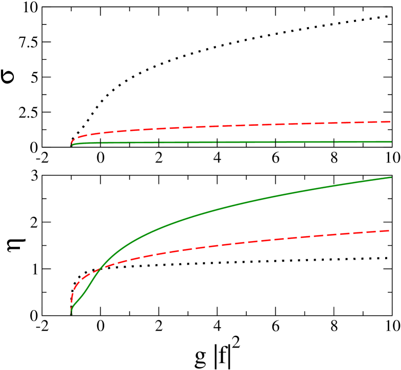
In Fig. 1 we report the transverse widths and obtained from Eqs. (23), (24) and the numerical solution of Eq. (25) with the Newton-Raphson method. We plot the widths as a function of the axial strength for three values of the transverse anisotropy .
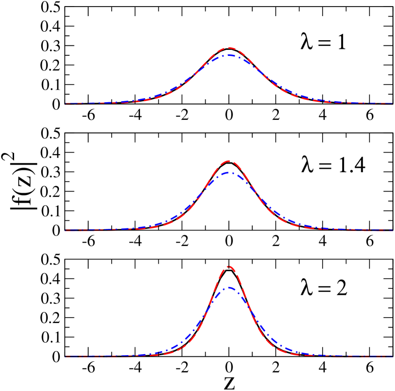
To test the accuracy of 1D g-NPSE we consider the case with negative scattering length () without axial confinement (). Under these conditions the system admits triaxial bright soliton configurations [13]. In Fig. 2 we plot the axial density profile of the BEC with and three values of the transverse anisotropy . The solid curves represent the numerical results obtained by solving the 3D GPE, Eq. (2), with a finite-difference Crank-Nicolson algorithm with imaginary time [14]. In this case the axial density profile is given by
| (26) |
with ground-state wave function of the 3D GPE. The dashed curves are obtained by solving the g-NPSE and the dot-dashed curves by the 1D GPE. The figure shows that the results of g-NPSE are in good agreement with the 3D GPE ones, while the predictions of the 1D GPE, Eq. (13), are not very reliable for the interaction strength .
3 1D generalized DNPSE
Let us consider again Eq. (2) where now the axial potential is given by
| (27) |
This potential models the optical lattice produced in experiments with Bose-Einstein condensates by using counter-propagating laser beams [15].
To symplify the problem we set
| (28) |
where is the Wannier function maximally localized at the -th minimum of the axial periodic potential. This tight-binding ansatz is reliable in the case of a deep optical lattice [15, 16]. We insert this ansatz into Eq. (2), multiply the resulting equation by and integrate over variable. In this way we get
| (29) |
where the parameters , and are given by
| (30) |
| (31) |
| (32) |
In the tight-binding regime the parameter is positive definite. In addition the parameters , and are independent on the site index .
Eq. (29) can be seen as the Euler-Lagrange equation of the following Lagrangian density
| (33) | |||||
To further simplify the problem we set
| (34) |
where , and , which account for discrete transverse widths and axial wave function, are the effective generalized coordinates to be determined variationally.
We insert this ansatz into the Lagrangian density (33) and integrate over and variables. In this way we obtain an effective Lagrangian for the fields and . This Lagrangian reads
| (35) | |||||
To obtain this expression we have supposed that the transverse widths of nearest-neighbor sites are practically equal (this is the equivalent to the adiabatic approximation made for the continuous model). The Euler-Lagrange equation of (35) with respect to is
| (36) | |||||
while the Euler-Lagrange equations of (35) with respect to and give
| (37) | |||
| (38) |
We call this system of coupled equations, which describe the BEC under a transverse anisotropic harmonic confinement and an axial optical lattice, the 1D generalized and discrete nonpolynomial Schrödinger equation NPSE (1D g-DNPSE) In the case of isotropic transverse harmonic confinement () we have
| (39) |
and the 1D g-DNPSE becomes
| (40) |
which is substantially the 1D DNPSE derived in Ref. [11].
4 Conclusions
We have obtained new nonpolynomial Schrödinger equations for matter waves under anisotropic transverse harmonic confinement. In the case of isotropic transverse confinement these continuous and discrete equations reduce to the ones derived in previous papers. The generalized 1D continuous nonpolynomial Schrödinger equation can be used to study the static and dynamics of Bose condensates with a generic longitudinal axial potential. The generalized 1D discrete nonpolynomial Schrödinger equation can be insead used to investigate the effect of a deep axial periodic potential. The comparison with the full 3D Gross-Pitaevskii equations show that these effective 1D equations are indeed quite accurate and much simpler for numerical and analytical computations.
The author thanks Alberto Cetoli, Boris Malomed, Giovanni Mazzarella, Dmitry Pelinovsky and Flavio Toigo for useful comments and suggestions. This work has been partially supported by Fondazione CARIPARO.
References
References
- [1] A.J. Leggett, Quantum Liquids. Bose Condensation and Cooper Pairing in Condensed-Matter Systems (Oxford Univ. Press, Oxford, 2006).
- [2] V. M. Pérez-García, H. Michinel, and H. Herrero, Phys. Rev. A 57, 3837 (1998).
- [3] A.D. Jackson, G.M. Kavoulakis, and C.J. Pethick, Phys. Rev. A 58, 2417 (1998).
- [4] L. Salasnich, A. Parola, and L. Reatto, Phys. Rev. A 65, 043614 (2002).
- [5] L. Salasnich, Laser Phys. 12, 198 (2002).
- [6] P. Massignan and M. Modugno, Phys. Rev. A 67, 023614 (2003); M. Modugno, C. Tozzo, and F. Dalfovo, Phys. Rev. A 70, 043625 (2004); C. Tozzo, M. Kramer, and F. Dalfovo, Phys. Rev. A 72 023613 (2005): M Modugno, Phys. Rev. A 73, 013606 (2006).
- [7] A.M. Kamchatnov and V.S. Shchesnovich, Phys. Rev. A 70 023604 (2004); D. E. Pelinovsky, P.G. Kevrekidis, D.J. Frantzeskakis, and V. Zharnitsky, Phys. Rev. E 70, 047604 (2004).
- [8] G. Theocharis, P. G. Kevrekidis, M. K. Oberthaler, and D. J. Frantzeskakis, Phys. Rev. A 76, 045601 (2007); A. Weller, J. P. Ronzheimer, C. Gross, J. Esteve, M. K. Oberthaler, D. J. Frantzeskakis, G. Theocharis, and P.G. Kevrekidis, Phys. Rev. Lett. 101, 130401 (2008).
- [9] A. Munoz Mateo and V. Delgado, Phys. Rev. A 75, 063610 (2007); A. Munoz Mateo and V. Delgado, Phys. Rev. A 77, 013617 (2008); A. Munoz Mateo and V. Delgado, Ann. Phys. 324, 709 (2009).
- [10] L. Salasnich, A. Parola, and L. Reatto, Phys. Rev. A 66, 043603 (2002); L. Salasnich, Phys. Rev. A 70, 053617 (2004); L. Salasnich, A. Parola and L. Reatto, Phys. Rev. A 70 013606 (2004); A. Parola, L. Salasnich, R. Rota, and L. Reatto, Phys. Rev. A 72, 063612 (2005); L. Salasnich and B.A. Malomed, Phys. Rev. A 74, 053610 (2006).
- [11] A. Maluckov, L. Hadzievski, B.A. Malomed, and L. Salasnich, Phys. Rev. A 78, 013616 (2008).
- [12] L. Salasnich and B.A. Malomed, Solitons and solitary vortices in “pancake”-shaped Bose-Einstein condensates, submitted for publication (2009).
- [13] L. Salasnich, Laser Phys. 15, 366 (2005).
- [14] E. Cerboneschi, R. Mannella, E. Arimondo, and L. Salasnich, Phys. Lett. A 249, 495 (1998); L. Salasnich, A. Parola, and L. Reatto, Phys. Rev. A 64, 023601 (2001).
- [15] O. Morsch and M. Oberthaler, Rev. Mod. Phys. 78, 179 (2006).
- [16] A. Trombettoni and A. Smerzi, Phys. Rev. Lett. 86, 2353 (2001); A. Smerzi and A. Trombettoni, P.G. Kevrekidis, and A.R. Bishop, Phys. Rev. Lett. 89, 170402 (2002); A. Smerzi and A. Trombettoni, Phys. Rev. A 68, 023613 (2003).