Generalized Spectral Coarsening
Abstract.
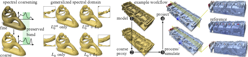
Many computational algorithms applied to geometry operate on discrete representations of shape. It is sometimes necessary to first simplify, or coarsen, representations found in modern datasets for practicable or expedited processing. The utility of a coarsening algorithm depends on both, the choice of representation as well as the specific processing algorithm or operator. e.g. simulation using the Finite Element Method, calculating Betti numbers, etc. We propose a novel method that can coarsen triangle meshes, tetrahedral meshes and simplicial complexes. Our method allows controllable preservation of salient features from the high-resolution geometry and can therefore be customized to different applications.
Salient properties are typically captured by local shape descriptors via linear differential operators – variants of Laplacians. Eigenvectors of their discretized matrices yield a useful spectral domain for geometry processing (akin to the famous Fourier spectrum which uses eigenfunctions of the derivative operator). Existing methods for spectrum-preserving coarsening use zero-dimensional discretizations of Laplacian operators (defined on vertices). We propose a generalized spectral coarsening method that considers multiple Laplacian operators defined in different dimensionalities in tandem. Our simple algorithm greedily decides the order of contractions of simplices based on a quality function per simplex. The quality function quantifies the error due to removal of that simplex on a chosen band within the spectrum of the coarsened geometry.
1. Introduction
Discrete representations of shape are ubiquitous across computer graphics applications. Meshes, a common choice for computer graphics applications, are specific instances of general abstractions called simplicial complexes. While the vertices of a mesh are commonly embedded (have explicit coordinates) in 2D or 3D, simplicial complexes capture abstract relationships between nodes – as extensions of graphs by including 3-ary (triangles), 4-ary (tetrahedra) and higher dimensional-relationships. We develop an algorithm to coarsen simplicial complexes of arbitrary dimensionality.
The choice of discretization has a profound impact on downstream applications that operate on the geometry, both in terms of efficiency as well as numerical stability. Simplification schemes are used to reduce the number of discrete elements while preserving quality. Quality can defined either in terms of aesthetic appeal (direct rendering, visualization, etc.) or functionally (finite element simulation, topological data analysis, geometry processing algorithms, etc.). We focus on the latter and propose a coarsening algorithm that can be tailored to different applications via a versatile definition of functionally salient features .
We resort to classical spectral theory to formalize the definition of qualities of the input representation which should be preserved while coarsening. Just as the famous Fourier spectrum is obtained via projection onto the eigenfunctions of the univariate derivative operator, our spectral domain of choice is defined via a projection onto a Laplacian operator. Unlike the univariate derivative operator, a variety of definitions exist for Laplacians. For discrete Laplacians, these usually arise from the elements of choice (vertices, edges, triangles, etc.) and their associated weights. The choice of the variant of Laplacian considered impacts the utility of the coarsened mesh in applications. For example, simplification of the domain of a physics simulation requires the preservation of the spectra of both 0- and 1-dimensional Laplacians (De Witt et al., 2012). The input to our algorithm includes a list of Laplacians and associated spectral bands – each band is a subspace in the spectrum corresponding to a Laplacian. Its output is a coarsened representation that preserves the spectral profile in the specified bands.
To summarize, we propose a coarsening algorithm for simplicial complexes that can preserve spectral bands of different Laplacians, across different dimensionalities of simplices. Our simple algorithm operates by first evaluating a quality function per simplex, which quantifies the error introduced by contracting (eliminating) that simplex towards the specified spectral band(s) to be preserved. Then, we greedily perform contractions iteratively by choosing candidates with minimum error until the target coarsening level is reached. Thus, our coarsening algorithm is agnostic to the specific Laplacian considered. Our contributions in this paper are:
-
•
a novel coarsening operator that is Laplacian-independent;
-
•
a coarsening operator that simultaneously preserves spectral bands associated with multiple Laplacians;
-
•
an algorithm for band-pass filtering of simplicial complexes.
We evaluate our method using a variety of surface (triangular) and volumetric (tetrahedral) meshes, as well as simplicial complexes.
2. Related Work
Graphs
The spectrum of a combinatorial graph Laplacian reveals fundamental geometric and algebraic properties of the underlying graph (Chung, 1999). Several works attempt to preserve spectral subspaces, while reducing the size of input graphs (Chen et al., 2022). A notable example (Loukas, 2019) proposes an iterative, parallelizable solution to preserve spectral subspaces of graphs by minimizing undesirable projections.
Meshes
Seminal works for coarsening triangle meshes propose localized and iterative operations via edge collapses based on visual criteria (Garland and Heckbert, 1997; Ronfard and Rossignac, 1996). Similar methods have also been applied to tetrahedral mesh simplification, based on volume, quadric-based, and isosurface-preserving criteria (Chopra and Meyer, 2002; Vo et al., 2007; Chiang and Lu, 2003). Recent methods formulate coarsening as an optimization problem subject to various sparsity conditions (Liu et al., 2019), by detaching the mesh from the operator (Chen et al., 2020) and localizing error computation to form a parallelizable strategy (Lescoat et al., 2020). The cotan Laplacian is a popular choice, and has also been used, via its functional maps, to identify correspondences between partial meshes (Rodolà et al., 2017) .
Simplicial complexes and computational topology
The link condition (Dey et al., 1998) is a combinatorial criterion ensuring that homology is preserved while performing strong collapses (merging vertices as opposed to edge removal), with extended applications and extensions to persistent homology (Wilkerson et al., 2013; Boissonnat and Pritam, 2019). Edge collapses in the form of edge removals (Boissonnat and Pritam, 2020; Glisse and Pritam, 2022) is a state-of-the-art method for simplifying filtered flag simplicial complexes while preserving their (persistent) homology. These methods focus on the dimensionality of the null space (kernel) of the Laplacian. They rarely investigate the general spectral profile of the reduced complex. Notable exceptions (Osting et al., 2017; Black and Maxwell, 2021; Hansen and Ghrist, 2019) apply the method of effective resistances (Spielman and Srivastava, 2011) for coarsening complexes, and cellular sheaves, respectively.
Spectral analysis
The Laplacian makes frequent appearances across geometry processing, machine learning and computational topology. Its specific definitions and flavours vary widely across domains, such as discrete exterior calculus (Desbrun et al., 2005; Crane et al., 2013), vector-field processing (Vaxman et al., 2016; Poelke and Polthier, 2016; de Goes et al., 2016; Wardetzky, 2020; Zhao et al., 2019b), fluid simulation (Liu et al., 2015), mesh segmentation and editing (Lai et al., 2008; Khan et al., 2020; Sorkine et al., 2004), topological signal processing (Barbarossa and Sardellitti, 2020), random walk representations (Lahav and Tal, 2020; Schaub et al., 2020), clustering and learning (Su et al., 2022; Nascimento and De Carvalho, 2011; Ebli and Spreemann, 2019; Ebli et al., 2020; Keros et al., 2022; Smirnov and Solomon, 2021). Its ability to effectively capture salient geometric, topological, and dynamic information of the object of interest makes its spectrum a versatile basis.
The de-facto Laplacian operator used in mesh processing is the Laplace-Beltrami operator which is approximated via a discretization called the cotan Laplacian defined on vertices (0D) with vertex and edge weights. A multitude of other Laplacians have been shown to accommodate non-manifold meshes (Sharp and Crane, 2020), FEM simulations (Ayoub et al., 2020), digital surfaces (Caissard et al., 2019), polygonal meshes (Bunge et al., 2021) and arbitrary simplicial complexes (Ziegler et al., 2022).
Motivation
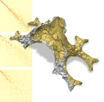
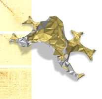
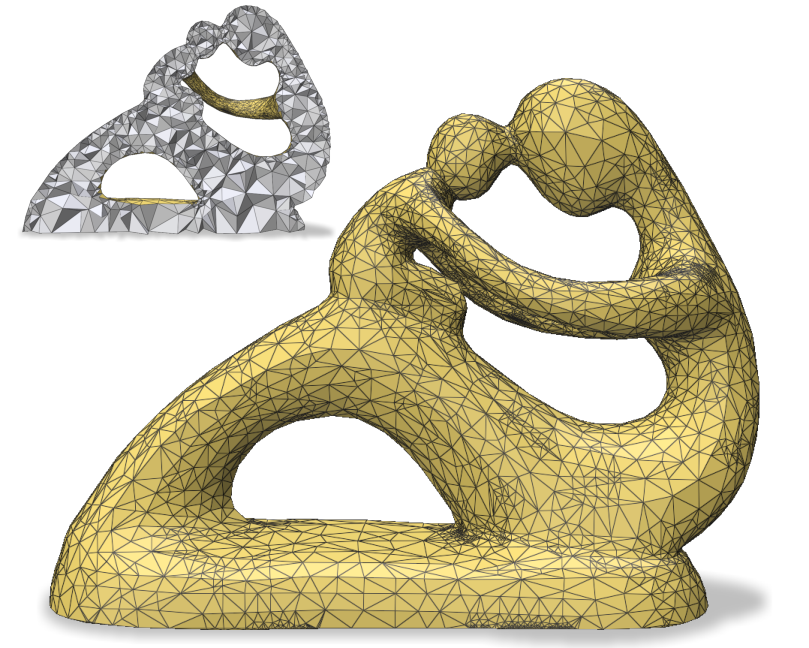
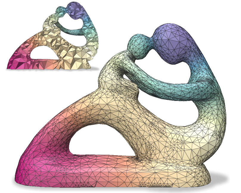
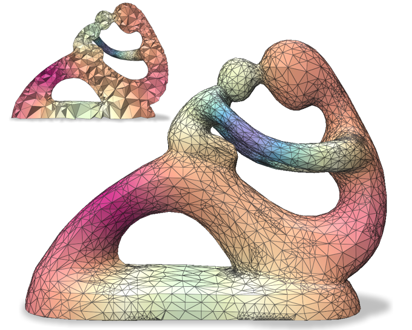
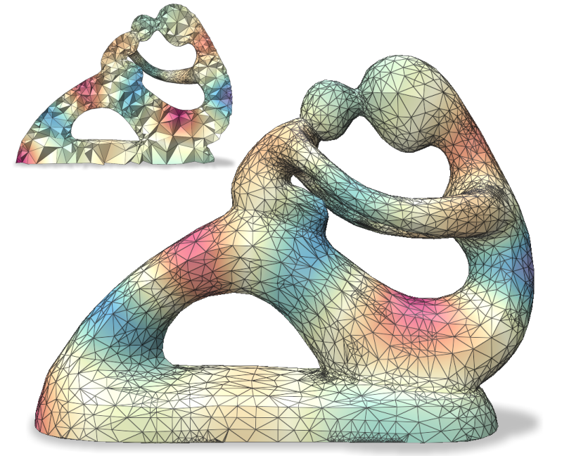
The variety of definitions and properties of Laplacian operators (see Figure 1) suggests that a unified spectral coarsening algorithm could impact a range of applications. Our Laplacian-agnostic spectral coarsening can be tailored by considering the weightings as special cases of Hodge Laplacians. We achieve this by adapting the cost function proposed for graph theory (2019) to simplicial complexes and incorporating it within a standard mesh-coarsening framework (Garland and Heckbert, 1997).
3. Background
3.1. Simplicial Complexes & Meshes
A simplicial complex is constructed by considering appropriate subsets of a finite set of vertices. Each element exists in as a singleton set . also contains which is called a -simplex of dimension . e.g. edges (), triangles (), tetrahedra (), etc. For every such , all of ’s subsets are also included in . The dimension of the simplicial complex is the maximal dimension of its simplices: . A graph is a 1-dimensional simplicial complex. Another well known special case is a triangle mesh , which is a 2-dimensional embedded simplicial complex often with additional manifold conditions on the adjacencies of 2-simplices (faces) . A tetrahedral mesh is a 3-dimensional embedded simplicial complex.
For a graph , the incidence matrix where (or ) depending on whether (or respectively) and zero otherwise, represents directed connectivity between vertices and edges. Boundary matrices extend this idea to higher dimensions and capture connectivity between (the vector space with real coefficients spanned by) the -simplices and their bounding simplices. For convenience boundary operators are constructed by imposing an ordering on the vertices , such that each -simplex can be expressed by an ordered list .
The orientation of the simplices in a simplicial complex is dictated by the ordering imposed on the vertices, and the orientation of mesh elements given by the cyclic ordering of vertices. The boundary action is then applied on each simplex according to where indicates the deletion of the -th vertex from , resulting in a -dimensional bounding simplex. The following figure illustrates a complex along with its three boundary matrices: white cells are zeros and grey cells are .
![[Uncaptioned image]](https://cdn.awesomepapers.org/papers/ec322b87-3642-401e-b28d-aa71f1b3c05e/x2.png)
3.2. Hodge Laplacian as a generalization
Hodge Laplacians (Rosenberg and Steven, 1997) are differential operators that extend the notion of the well-known graph and mesh Laplacians to higher-dimensional simplicial complexes. It is defined, for each dimension , as the sum of a two maps from -simplices: one mapping down to -simplices and another mapping up to -simplices. Each map is defined via its appropriate boundary matrix:
are diagonal matrices that contain a weight per simplex. The superscript clarifies that is the random walk -Hodge Laplacian – an antisymmetric linear map from -simplices to -simplices. It can be symmetrized, while preserving its spectral properties, as . We direct the reader to key works (Horak and Jost, 2013; Lim, 2020) that present a thorough treatment of Hodge Laplacians and their spectra. We refer to as the weighted -Hodge Laplacian and to its unweighted (unit weights) version as simply the -Hodge Laplacian.
Most variants of Laplacians used in graph- and mesh-processing may be derived as special cases of the weighted -Hodge Laplacian. The graph Laplacian is a 0-Hodge Laplacian with unit weight on vertices . The cotan Laplacian, popular as the stiffness matrix in finite element methods, is the 0-Hodge Laplacian with different weights assigned to vertices and edges:
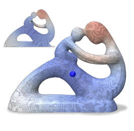
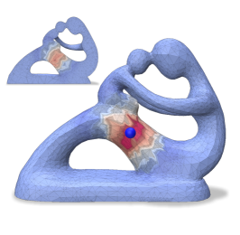
is the area of face , and is the angle at vertex facing the edge . Figure 1 (left) depicts the impact of the choice of Laplacian on the coarsened Fertility triangle mesh.
Hodge Spectra
Every basis of the vector space of a complex is spanned by a representative of equivalence classes of -dimensional nontrivial loops, and is isomorphic to the kernel of the -Hodge Laplacian (Eckmann, 1944): . The eigenvectors of corresponding to zero eigenvalues (the harmonic part of the spectrum) are minimal representatives of their respective homology classes. An eigenvector corresponding to a non-zero eigenvalue of , must either be an eigenvector of or with the same eigenvalue. Furthermore, an element of the nullspace of must be in the kernel of both of its components. Given an eigenpair of then is an eigenpair of (Torres and Bianconi, 2020; Horak and Jost, 2013). The Hodge decomposition ties everything together, by expressing the space of -simplices as a direct sum of gradients, curls, and harmonics:
We refer to several excellent introductions (Lim, 2020; Chen et al., 2021) to Hodge decompositions.
4. Method
We propose a simple iterative algorithm for coarsening a simplicial complex based on two inputs: the fraction of simplices to be reduced and the portion of the input spectrum needing to be preserved. We use the latter to construct a quality function that is evaluated at each simplex. Then we greedily contract a simplex (or a group of simplices with low spectral-quality scores). We recalculate the quality function for simplices in the coarsened complex and iterate until the specified number of simplices have been reduced.
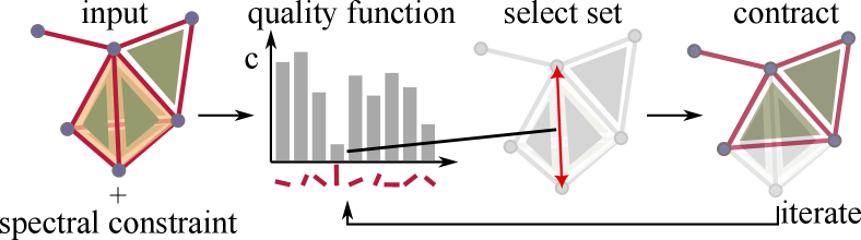
4.1. Quality function
Each contraction (e.g. edge collapse) can be defined as a projection mapping -simplices in the input complex to those in the coarsened complex. Ideally, the eigenspace to be preserved should be perpendicular to that induced by the contraction. Intuitively the projection of the former onto the latter measures “spectral leak”, with a large value indicating that the contraction leads to loss of fidelity with respect to the specified target spectrum.
Let the eigenspace to be preserved be represented by eigenvectors and eigenvalues (diagonal matrix) of the Hodge Laplacian (or ) of the input complex, and let be the preserved subspace. Since and its pseudoinverse , where is a diagonal (normalizing) matrix containing row norms, map in opposite directions to and from the output complex, the operator projects a signal defined on the fine complex down to the coarsened complex and back up to the fine complex.
Ideally, we seek contractions where is identical to by minimizing . Our quality function
| (1) |
where the perpendicular projection , quantifies spectral error. Here denotes the -norm. The above definition of in terms of allows for localized error computations, facilitating parallelization, since the nonzero entries of only refer to simplices affected by the contraction. This quality function, has been analyzed to have desirable theoretical properties when applied to graph simplification and general positive semidefinite matrices (Loukas, 2019).
4.2. Contraction
The first step to performing contractions, or setting equivalences of multiple simplices, is to identify a set of candidate contraction sets . We execute edge collapses by setting each to be an edge. More complicated contractions, such as collapsing stars around vertices, may be performed by identifying the relevant .
Then, we evaluate the quality function over each candidate contraction set and greedily contract the set with the minimum quality. This involves identifying all the simplices in to one, target, vertex. As a result, the complex is coarsened while best preserving the spectral band of . In practice, we apply such contractions iteratively until a specified ratio of simplices has been contracted, with some additional bookkeeping at each level : starting from , we update the target subspace and the corresponding projection matrices and , with tracking the evolution of the desired spectrum at each iteration.
4.3. Multiple Laplacian subspaces
The quality function (Equation 1) can be adapted so that the target subspace is shaped via multiple spectral bands. We define cost functions at level independently for different spectral bands . Each of these is associated with a potentially different Laplacian. The aggregate cost function can then be tailored based on the specific downstream application as to obtain the final quality function
In our experiments in Section 5, where , and are considered in tandem, we simply average the contributions of the different Laplacians . Algorithm 1 shows our generalized coarsening procedure by assembling the above stages.
4.4. Implementation details
Terms of the Hodge Laplacian
Due to the interplay of spectra of and discussed in Section 3.2, constraints on Laplacians for multiple can potentially introduce ‘spectral conflicts’. We avoid this by considering only the components of the chosen Laplacians for each . For wide spectral bands and appropriate choice of , the spectral region of interest will be a subspace of the spectrum of and thus preserved.
Building coarsening matrices
During contraction, let be the index of a contracted simplex in , be the index of the target simplex in and bet the cardinality of the candidate family being contracted. is then a simplicial map where every simplex of maps to a valid simplex of , or to zero. For consistency, it is required that . To satisfy desirable spectral approximation guarantees (Loukas, 2019) and for to hold, we set the elements of each contraction set as , for all , where . We resolve the ambiguity of the choice of target simplex by consistently selecting the target simplex based on its index. e.g. for edge contractions, both vertices are merged into one with the smaller index.
Choosing candidate families
Our algorithm is agnostic of the choice of combinations of simplices to be contracted. We tested with various candidate families: edges (pairs of vertices), faces (triplets of vertices) and more general vertex neighborhoods consisting of closed-stars. Larger contraction sets result in aggressive coarsening at each iteration which leads to larger spectral error. All results in this paper use only edge collapses. This also simplifies comparison to related work (which are restricted to edge collapses).
Harmonic subspaces
For , the harmonic portion of the spectrum of is non-trivial and encodes information about non-trivial cycles called homology generators. A homology group is a vector space of cycles that are not bounding higher dimensional simplices and therefore manifest as the null space of . It is often desirable to preserve these eigenvectors, despite their coresponding zero eigenvalue, to maintain topological consistency. In practice, for all experiments we use modified eigenvalues when dealing with spectral of higher-dimensional Laplacians.
Local Delaunay vertex position optimization
Edge contractions may produce self-intersections, particularly if a fixed vertex-placement policy is followed, say, at the midpoint of an edge. While there are methods to avoid this effectively (Sacht et al., 2013), we adopted a simple vertex positioning scheme for tetrahedral meshes to prevent intersections.
![[Uncaptioned image]](https://cdn.awesomepapers.org/papers/ec322b87-3642-401e-b28d-aa71f1b3c05e/x4.png)
Our scheme operates in four steps: (1) identify the faces in the link of the edge being collapsed; (2) construct the Delaunay tetrahedralization of the vertices of these faces; (3) choose barycenters of the new tetrahedra that are on the same side of the faces in 1 as the corresponding vertex of the edge being collapsed; (4) the output vertex is the centroid of all vertices that pass the test in 3. If no vertices pass the test in 3 then we do not perform the collapse.
| Ref . (11385 v.) | 5000 verts. | 3000 verts. | 1000 verts. |
 |
 |
 |
 |
| 5000 v. | 0 | 39.126 | 1.023 | 7.855 | 0.010 | 13.8 | 9.07 |
| 1 | 73.351 | 0.007 | 1.251 | 0.183 | 8.4 | 5.165 | |
| 2 | 83.015 | 0.003 | 1.241 | 0.174 | 2.95 | 2.52 | |
| 3000 v. | 0 | 61.272 | 3.298 | 13.506 | 0.002 | 8.17 | 19.51 |
| 1 | 91.813 | 0.013 | 1.723 | 0.381 | 2.48 | 10.138 | |
| 2 | 97.56 | 0.004 | 1.583 | 0.489 | 0.44 | 4.89 | |
| 1000 v. | 0 | 87.90 | 8.266 | 26.511 | 0.009 | 2.45 | 55.53 |
| 1 | 97.72 | 0.026 | 2.804 | 0.532 | 0.75 | 23.139 | |
| 2 | 99.60 | 0.011 | 2.434 | 0.709 | 0.07 | 11.34 |
| triangle mesh | |||||||
| ours | 0 | 9.94 | 37.314 | ||||
| baseline | 0 | 4738 | 5648 | ||||
| ours | 1 | 31.35 | 0.350 | 0.590 | |||
| baseline | 1 | 0.018 | 0.827 | 2.555 | 0.635 | ||
| tetrahedral mesh | |||||||
| ours | 0 | 22.379 | 142 | 130 | 24.58 | 1.827 | |
| ours | 1 | 83.90 | 0.030 | 2.206 | 0.174 | 4.999 | 9.581 |
| ours | 2 | 91.14 | 0.007 | 1.696 | 0.287 | 1.289 | 1.938 |
5. Results
Unless otherwise specified, we use a common low-pass constraint as the default for experiments: to preserve the space spanned by the first eigenvectors of the specified Laplacian(s).
5.1. Meshes
2D Baseline
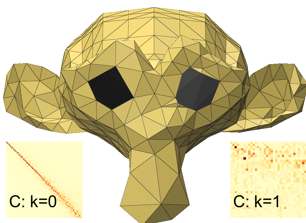
To enable comparisons of for triangle meshes we extend previous work (Lescoat et al., 2020) as a baseline. Their method minimizes spectral error where is a coarsening projection matrix, is a mass matrix, is a differential operator, and is the spectrum of interest as a matrix of eigenvectors. A tilde above the respective notations denotes their coarsened versions. From their output coarsening matrix we additionally infer coarsening matrices and which operate on the space of edges and faces respectively. However, they do not consider higher dimensional mappings in their error metric. Since they only consider one Laplacian , we include this as one of the targets in all our comparisons, unless stated otherwise. We visualize spectral preservation via functional maps (Liu et al., 2019; Lescoat et al., 2020; Chen et al., 2020) which is a diagonal matrix when the input and output spectra match perfectly. Unfortunately, it is not straightforward to compare with prior non-spectal tetrahedral coarsening methods, or to extend previous spectral coarsening methods to operate on tetrahedral meshes (Section 2).
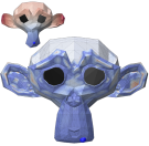
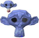
Quantitative comparison
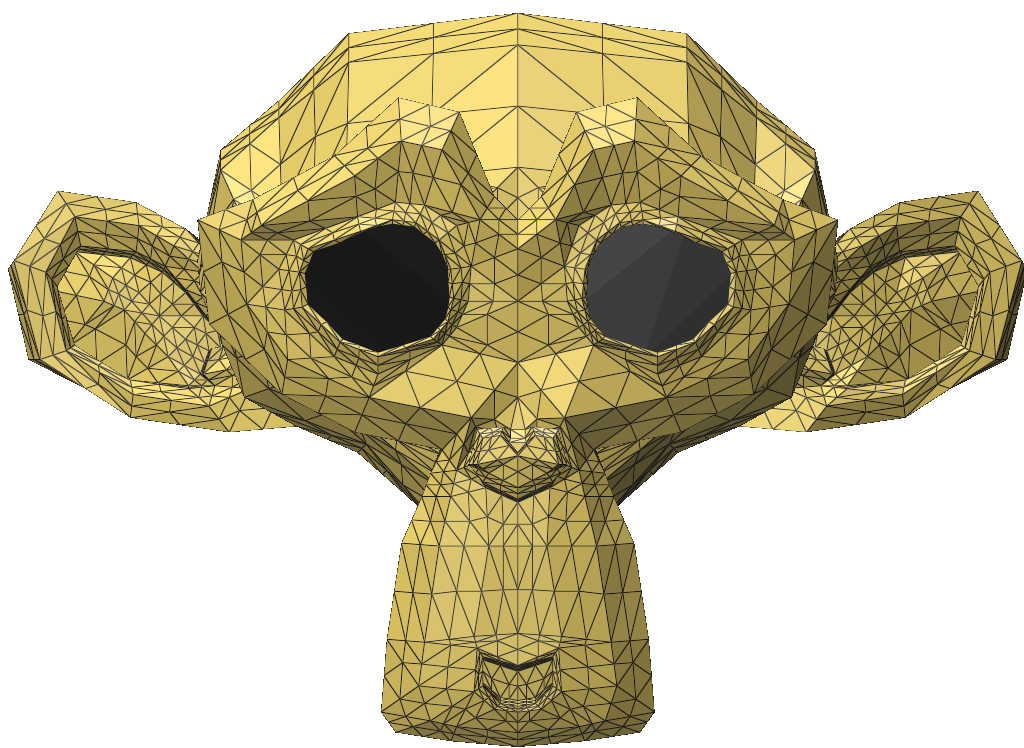
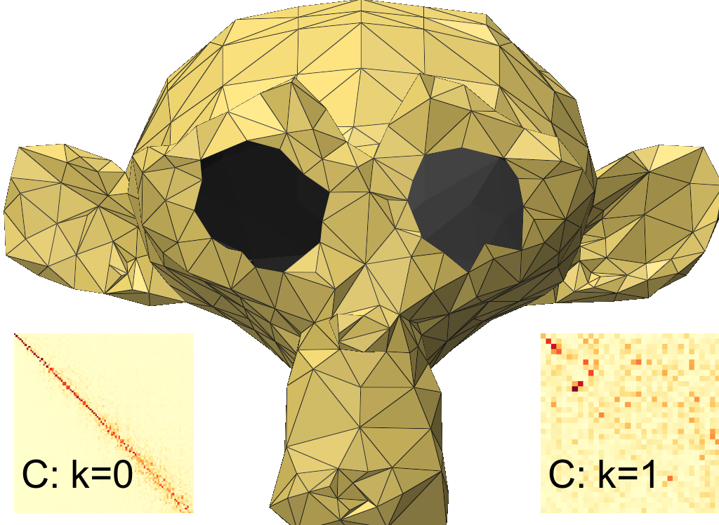
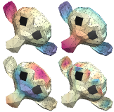
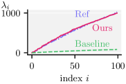
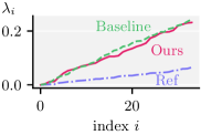
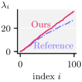
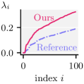
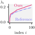
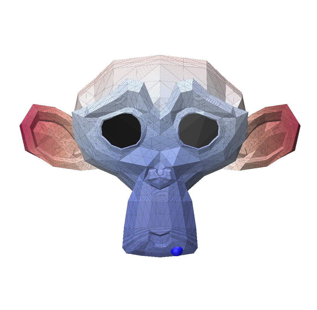
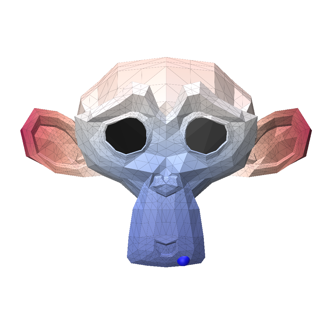
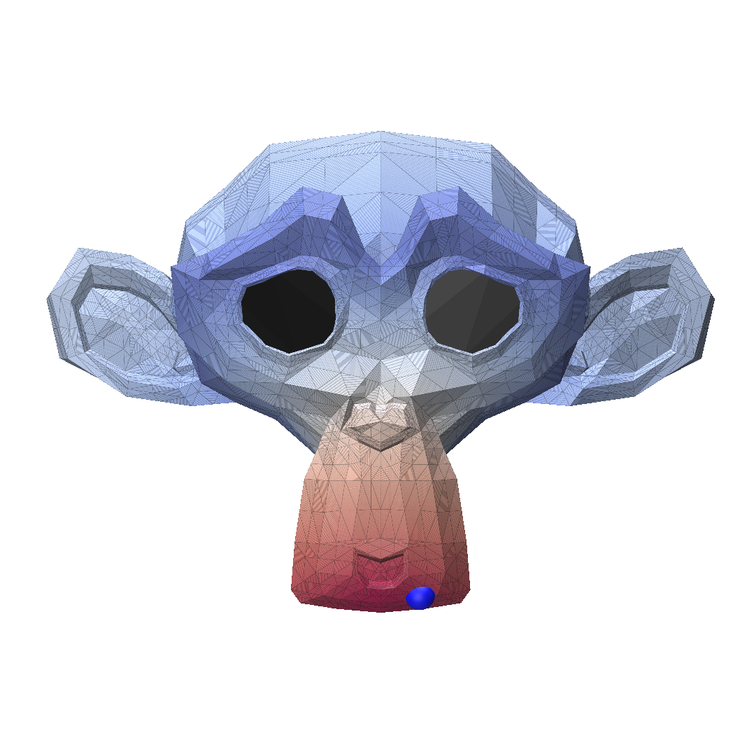
We visualize coarsened triangular (Figure 8) and tetrahedral (Figure 11) meshes along with a few eigenvectors (as heat maps on vertices). The results are reassuring that for the special case of coarsening triangle meshes our algorithm produces similar spectral results to previous work. Using subtly improves the preservation of structures such as the jaw-line, the mouth and the nose of the Suzanne model (Figure 8). The boundary loops around the eyes (eigenvectors of the null space of ) aim to preserve their original size compared to when only is used. The bottom row of Figure 8 contains quantitative comparisons of our eigenvalues against the baseline and reference. It appears that the approximation is good for , but curiously spectral divergence is observed for our method and the baseline in .
This is also observed on a tetrahedral mesh (Fertility model) as shown in the bottom row of Figure 9. However, the profile of eigenvalues for and the eigenvalues of are approximated well. We also show functional maps to support these observations. The Laplacians considered were and for the triangle mesh (2D), and additionally for the tetrahedral mesh. We report errors in Table 4 using the following error metrics: a local volume-preserving measure , an isometry measure , a conformality measure , a subspace approximation measure , subspace alignment and relative eigenvalue error .
The above results indicate comparable performance against the baseline for for triangle meshes and the added capability of handling higher dimensional Laplacians for tetrahedral (3D) meshes. Additional examples are included in the supplementary material. We illustrate the evolution of spectral errors for the Tree root model over three levels of coarsening (Figure 3).
5.2. Simplicial Complexes
We compare our coarsening algorithm to the state-of-the-art edgecollapser of the Gudhi library (The GUDHI Project, 2015), that guarantees homology preservation, and a simple baseline where edges are collapsed at random.
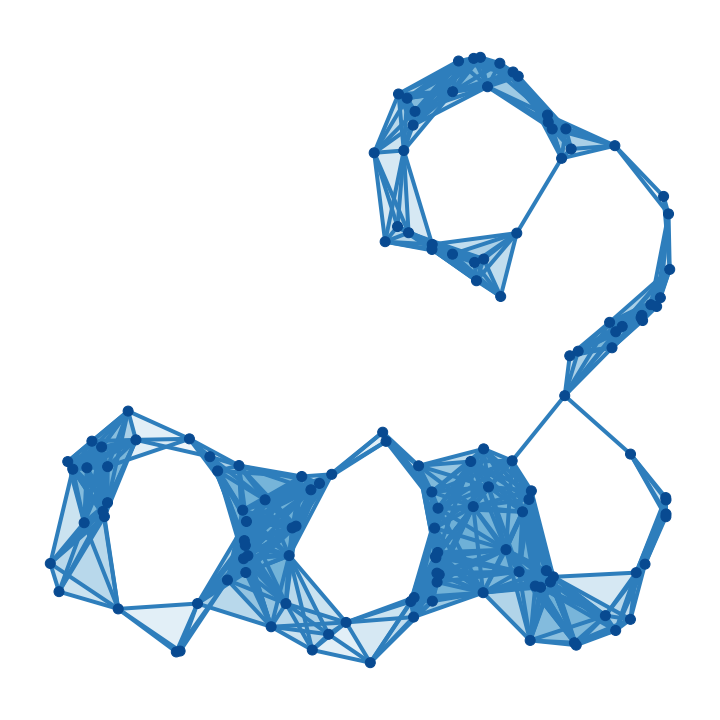
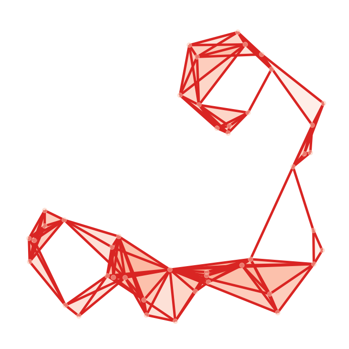
Band-pass filtering
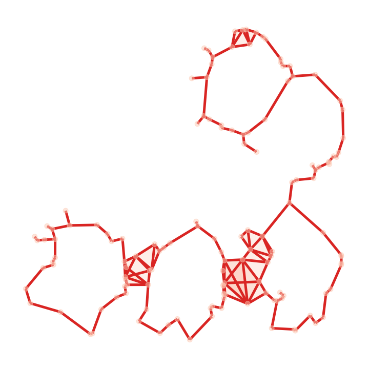
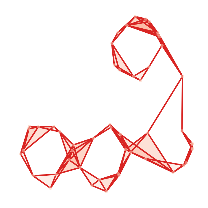
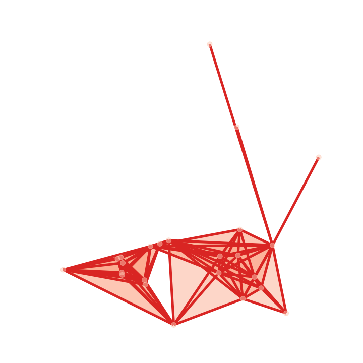
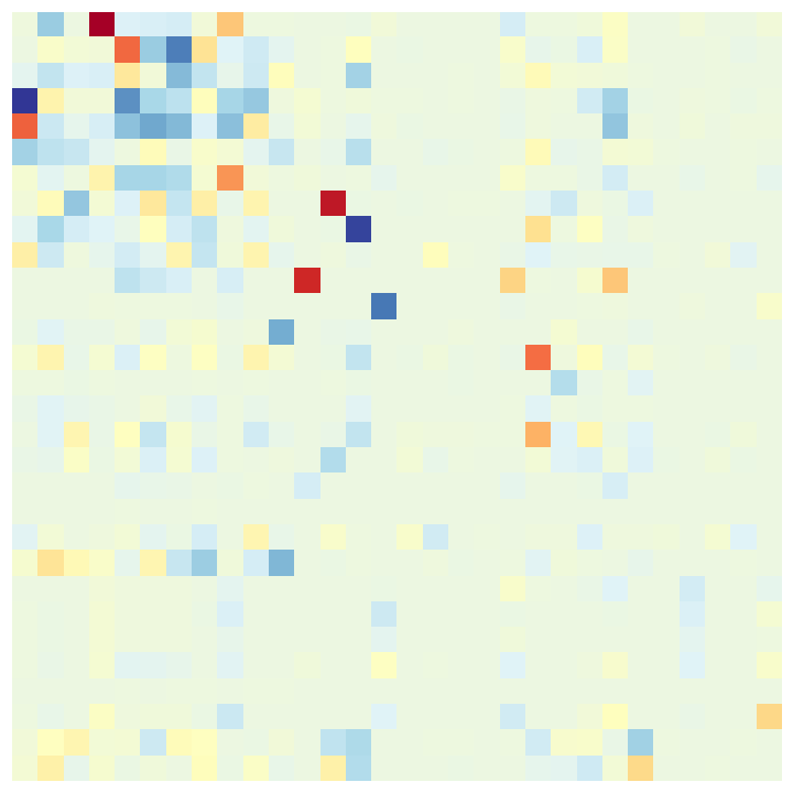
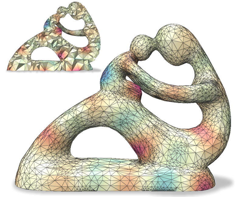
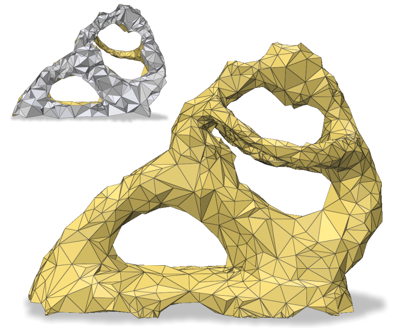
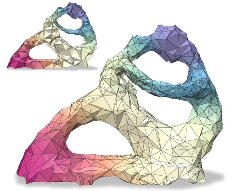
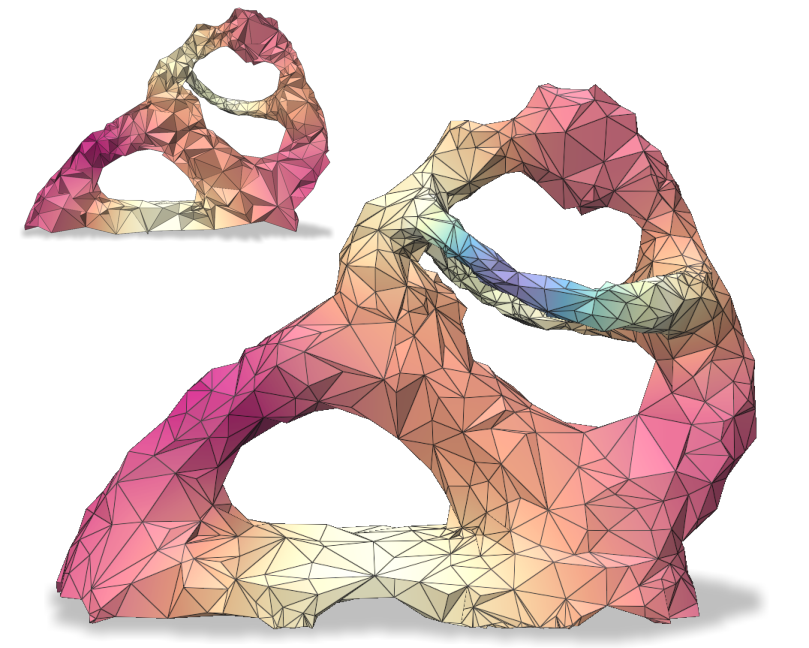
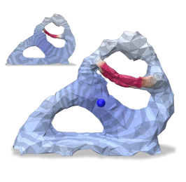
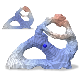
We demonstrate the versatility of our method by coarsening an input complex with two different spectral bands to be preserved: lowest, and 10 largest eigenpairs of . Here, is the betti number (rank of the homology group ). Figure 5 presents these results along with the functional maps as explained above. As expected (by design), Gudhi exactly preserves the homology rank , with no regard for other features. On the contrary, our method can be tuned to a spectral band of choice. Either the nullspace-encoded harmonic information (first row of functional maps) or the high frequency band(second row of maps).
Homology preservation
We constructed a diverse dataset of 100 simplicial complexes (Keros et al., 2022) with non-trivial topology by randomly sampling 400 points repeatedly on multi-holed tori, and subsequently constructing alpha complexes at various thresholds. It contains from zero up to 66 homology cycles. On this dataset, we computed mean spectral error metrics (Table 1), alongside a homology preservation error . Intuitively, this is the error in the number of 1-cycles destroyed by coarsening. The number of simplices reduced by Gudhi was consistent across both experiments. We ran two variants of our method which preserved the first eigenpairs of , reducing the input complexes by a factor of 0.8, and the first eigenpairs of , matching the target number of vertices to the result of Gudhi. The results are summarized in Table 1 with standard deviations in parentheses. Gudhi, as designed, preserves exactly but exhibits spectral leak elsewhere. With random contractions, the leak is amortized across spectral bands but it destroys about 1 cycle on average. Our method is controllable, highlighting that it can be particularly effective if the spectral constraints are known for a particular application.
| k | |||||||
| 30 | Gudhi | 0.9 | 3.84 (4.2) | 29.1 ( 2.9) | 2.5 (16.8) | 71.5 (664) | 0.0 (0.0) |
| Ours | 0.8 | 0.49 (0.5) | 8.98 (3.5) | 1.52 (12.2) | 2.76 (10.5) | 0.07 (0.2) | |
| Random | 0.8 | 3.08 (2.2) | 20.8 (3.5) | 0.32 (0.4) | 400000 (3 e6) | .98 (1.2) | |
| Gudhi | 0.9 | - | 2.94 (1.0) | 0.91 (0.2) | - | 0.0 (0.0) | |
| Ours | 0.9 | - | 1.78 (1.2) | 0.78 (0.3) | - | 0.21 (0.6) | |
| Random | 0.9 | - | 2.76 (1.1) | 0.88 (0.2) | - | 1.29 (1.4) |
| Input | Random | Gudhi | Ours (low) | Ours (high) |
 |
 |
 |
 |
 |
|
0-10 |
 |
 |
 |
 |
|
790-800 |
 |
 |
 |
 |
5.3. Applications
Denoising
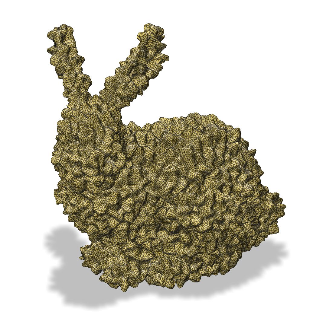
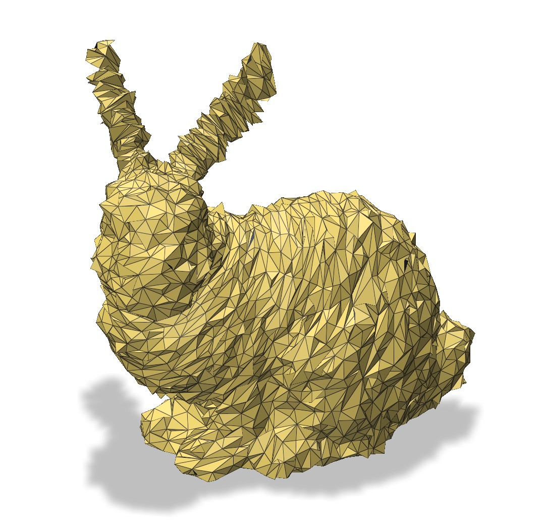
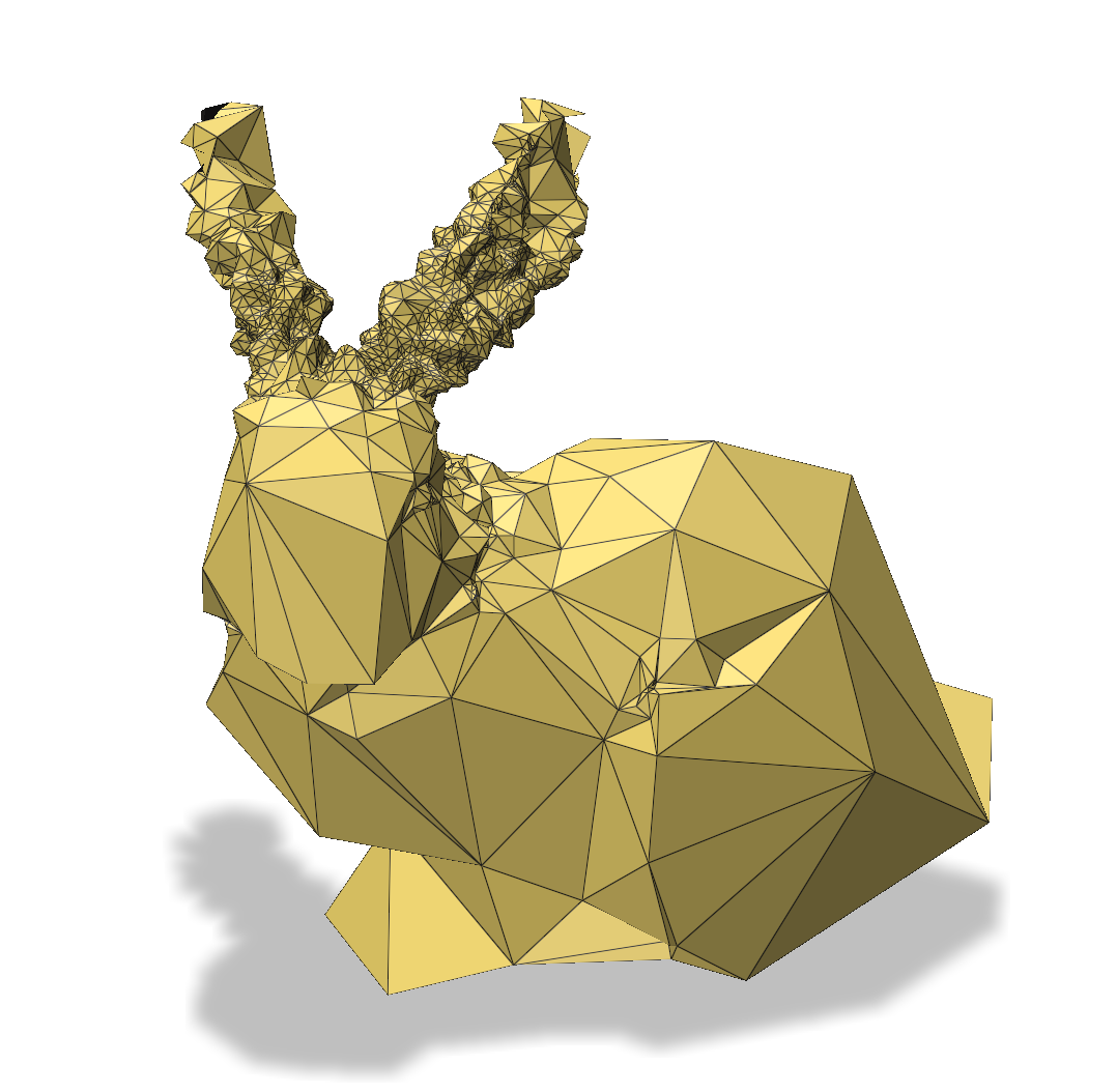
A straightforward application of our method is to suppress frequencies associated with noise. We filtered a noisy Bunny model (43K vertices) using a very narrow low-pass filter: only the first three eigenvectors of and . Figure 6 visualizes our result along with the baseline filters unevenly, possibly due to noisy geometric information in its cotan weighting.
| noisy | ours | baseline |
 |
 |
 |
Finite Element Method (FEM)
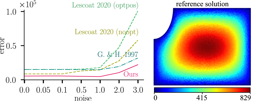
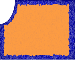
We solve the Poisson equation with Dirichlet boundary condition on the popular Plate-hole model, using piece-wise linear (triangular) elements. In addition to solving it on the discretized mesh, we test robustness by applying planar pertubations to the vertices with increasing levels of Gaussian noise. For each setting, we coarsen the noisy mesh with (8000 to 2000 vertices) using and , run a standard FEM solver on the coarse mesh and lift the solution to the input mesh. Figure 10 shows a plot of error vs noise (top left), the reference solution (top right) and error maps for different noise settings (columns) and methods (rows). Also shown are previous work (Lescoat et al., 2020), with (optpos) and without (noopt) vertex position optimization, and a quadric-based method (Garland and Heckbert, 1997). The coarse mesh is overlaid on the error maps and can be viewed by magnifiying the figure. Our method exhibits robustness against noise and improved approximation performance against element reduction.
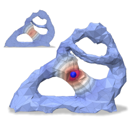
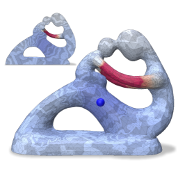
Spectral distances
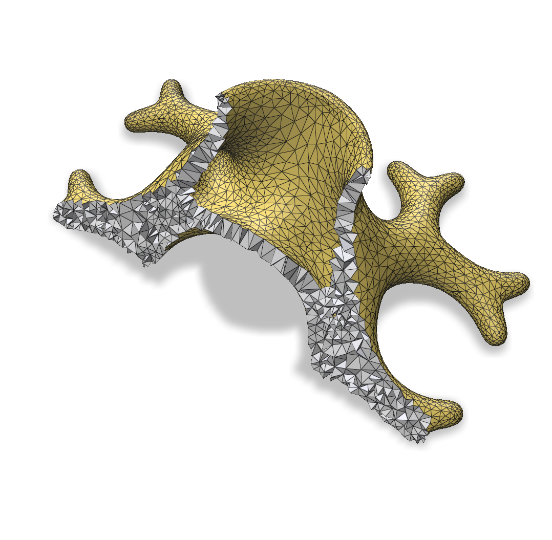
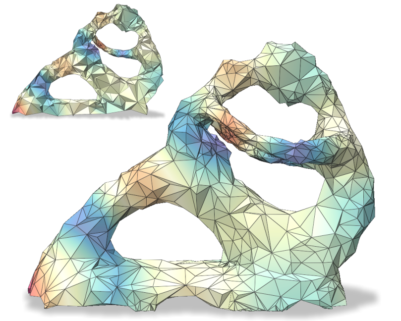
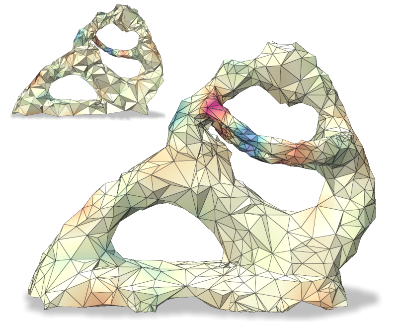
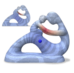
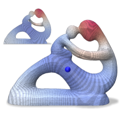
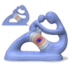
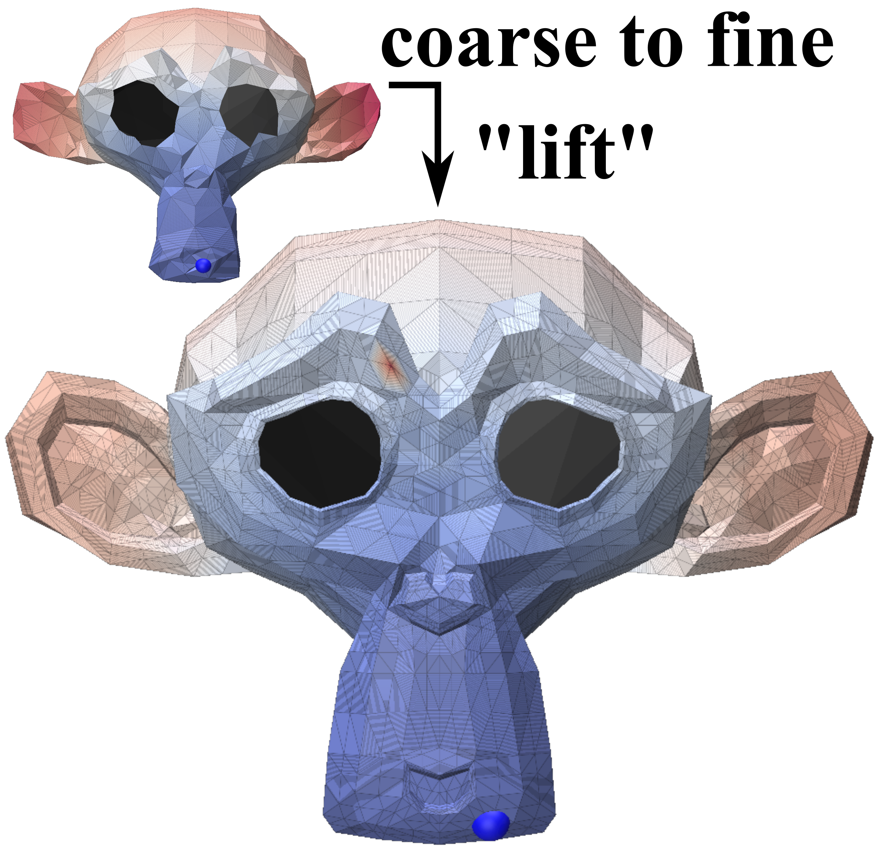
We evaluate the fidelity (Figure 12) of spectral distance measures computed on the coarse mesh and “lifted” to the fine mesh, between vertices of a triangle surface mesh (Suzanne) and a volume tetrahedral mesh (Fertility), using the same parameters as Figures 8 and 11. Figure 1 illustrates the spectral distance approximation process on the Engine tetrahedral model, coarsened with (from 46220 to 10000 vertices) while preserving the first 50 eigenvectors of and the first 25 eigenvectors of and . The model has 20 holes that are retained in the coarse mesh. The metrics used and their parameters are tabulated below.
| diffusion | ||
| biharmonic | ||
| commute | ||
| WKS | ||
| WKD | , | |
| HKS |
Spectral distance approximation on Suzanne outperforms the baseline by orders on magnitude in most cases, with error remaining low even for the tetrahedral Fertility mesh. The qualitative comparison indicates agreement between our “lifted” version and the reference, despite some localized distortions.
6. Discussion
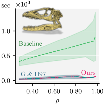
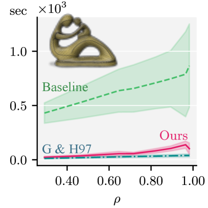
Execution time
We implemented our method in C++, and performed experiments on a 16-core workstation (Intel E5-2630 v3,2.4 GHz) with 64GB RAM. Our method compares favorably (orders of magnitude faster) against the spectral coarsening baseline in Figure 7. Although it appears that we are competitive with the quadric-based method (Garland and Heckbert, 1997)) it should be noted that ours (like the baseline) requires an eigenspace of the laplacians as input while the latter does not. The time for the eigendecomposition is not reflected in the plot (which only measures geometric operations) and should be added to both our method and the baseline. The triangle meshes used in the comparison contain 10772 (Fertility) and 29690 (Dinoskull) vertices, respectively. We use for the baseline, and & for our method.
 |
 |
Boundary
The intricacies of boundary values problems involving Hodge Laplacians (Mitrea, 2016) complicate practical computations. The differential operators need to be constructed carefully to guarantee coverage of tangential and normal conditions (Zhao et al., 2019a). Since our method is Laplacian-agnostic, any positive semi-definite variante of the Laplacian operator, with its spectrum, can be provided as input.
Limitation and future work
The utility of our tool hinges on knowledge of spectral constraints imposed by downstream tasks. While this is known in some cases (homology, spectral distances and denoising), such constraints are not typically known across applications. There is especially little use of higher dimensional Laplacian operators. However, we are hopeful that the availability of a tool such as ours will inspire the graphics communities (particularly geometry processing and simulation) to explore the applicability of mixed-dimensional Laplacian spectral constraints.
7. Conclusion
We presented a simple and efficient algorithm for coarsening simplicial complexes, while preserving targeted spectral subspaces across multiple dimensions. We exemplified the impact of the choices of spectral domain on applications such as denoising, FEM and approximate distance calculations on coarsened meshes. We hope that this work will pave the way towards unleashing the potential of using mixtures of Laplacians in discrete geometry processing.
|
Reference |
|
|
|
Ours |
|
|
|
Baseline |
|
|
 |
 |
 |
 |
 |
 |
 |
 |
| Error maps | |||
|
Ours |
 |
 |
 |
|
L. 2020 (noopt) |
 |
 |
 |
|
G& H 97 |
 |
 |
 |
| noise = 0.0 | noise = 1 | noise = 3 | |
|
Reference |
 |
 |
 |
 |
 |
|
Ours |
 |
 |
 |
 |
 |
| 2D (triangle mesh) | 3D (tetrahedral mesh) | ||||||||||||||||||||||||||||||||||||||||||||
| Diffusion | Biharmonic | HKS | Diffusion | Biharmonic | HKS | ||||||||||||||||||||||||||||||||||||||||
|
Reference |
 |
 |
 |
Reference |
 |
 |
 |
||||||||||||||||||||||||||||||||||||||
|
Ours |
 |
 |
 |
Ours |
 |
 |
 |
||||||||||||||||||||||||||||||||||||||
|
Baseline |
 |
 |
 |
Ours - Lifted |
 |
 |
 |
||||||||||||||||||||||||||||||||||||||
|
|
||||||||||||||||||||||||||||||||||||||||||||
References
- (1)
- Ayoub et al. (2020) Rama Ayoub, Aziz Hamdouni, and Dina Razafindralandy. 2020. A new Hodge operator in Discrete Exterior Calculus. Application to fluid mechanics. arXiv preprint arXiv:2006.16930 (2020).
- Barbarossa and Sardellitti (2020) Sergio Barbarossa and Stefania Sardellitti. 2020. Topological signal processing over simplicial complexes. IEEE Transactions on Signal Processing 68 (2020), 2992–3007.
- Black and Maxwell (2021) Mitchell Black and William Maxwell. 2021. Effective Resistance and Capacitance in Simplicial Complexes and a Quantum Algorithm. In 32nd International Symposium on Algorithms and Computation (ISAAC 2021) (Leibniz International Proceedings in Informatics (LIPIcs), Vol. 212), Hee-Kap Ahn and Kunihiko Sadakane (Eds.). Schloss Dagstuhl – Leibniz-Zentrum für Informatik, Dagstuhl, Germany, 31:1–31:27. https://doi.org/10.4230/LIPIcs.ISAAC.2021.31
- Boissonnat and Pritam (2019) Jean-Daniel Boissonnat and Siddharth Pritam. 2019. Computing Persistent Homology of Flag Complexes via Strong Collapses. In SoCG 2019-International Symposium on Computational geometry.
- Boissonnat and Pritam (2020) Jean-Daniel Boissonnat and Siddharth Pritam. 2020. Edge collapse and persistence of flag complexes. In SoCG 2020-36th International Symposium on Computational Geometry.
- Bunge et al. (2021) A. Bunge, M. Botsch, and M. Alexa. 2021. The Diamond Laplace for Polygonal and Polyhedral Meshes. Computer Graphics Forum 40, 5 (Aug. 2021), 217–230. https://doi.org/10.1111/cgf.14369
- Caissard et al. (2019) Thomas Caissard, David Coeurjolly, Jacques-Olivier Lachaud, and Tristan Roussillon. 2019. Laplace–beltrami operator on digital surfaces. Journal of Mathematical Imaging and Vision 61, 3 (2019), 359–379.
- Chen et al. (2020) Honglin Chen, Hsueh-TI Derek Liu, Alec Jacobson, and David I. W. Levin. 2020. Chordal Decomposition for Spectral Coarsening. 39, 6, Article 265 (nov 2020), 16 pages. https://doi.org/10.1145/3414685.3417789
- Chen et al. (2022) Jie Chen, Yousef Saad, and Zechen Zhang. 2022. Graph coarsening: from scientific computing to machine learning. SeMA Journal (2022), 1–37.
- Chen et al. (2021) Yu-Chia Chen, Marina Meilă, and Ioannis G Kevrekidis. 2021. Helmholtzian Eigenmap: Topological feature discovery & edge flow learning from point cloud data. arXiv preprint arXiv:2103.07626 (2021).
- Chiang and Lu (2003) Yi-Jen Chiang and Xiang Lu. 2003. Progressive Simplification of Tetrahedral Meshes Preserving All Isosurface Topologies. Computer Graphics Forum 22, 3 (Sept. 2003), 493–504. https://doi.org/10.1111/1467-8659.00697
- Chopra and Meyer (2002) Prashant Chopra and Joerg Meyer. 2002. Tetfusion: an algorithm for rapid tetrahedral mesh simplification. In IEEE Visualization, 2002. VIS 2002. IEEE, 133–140.
- Chung (1999) F R K Chung. 1999. Spectral Graph Theory. ACM SIGACT News 30 (1999), 14. https://doi.org/10.1145/568547.568553
- Crane et al. (2013) Keenan Crane, Fernando De Goes, Mathieu Desbrun, and Peter Schröder. 2013. Digital geometry processing with discrete exterior calculus. In ACM SIGGRAPH 2013 Courses. 1–126.
- de Goes et al. (2016) Fernando de Goes, Mathieu Desbrun, and Yiying Tong. 2016. Vector Field Processing on Triangle Meshes. In ACM SIGGRAPH 2016 Courses (Anaheim, California) (SIGGRAPH ’16). Association for Computing Machinery, New York, NY, USA, Article 27, 49 pages. https://doi.org/10.1145/2897826.2927303
- De Witt et al. (2012) Tyler De Witt, Christian Lessig, and Eugene Fiume. 2012. Fluid Simulation Using Laplacian Eigenfunctions. ACM Trans. Graph. 31, 1 (Jan. 2012), 1–11. https://doi.org/10.1145/2077341.2077351
- Desbrun et al. (2005) Mathieu Desbrun, Anil N Hirani, Melvin Leok, and Jerrold E Marsden. 2005. Discrete exterior calculus. arXiv preprint math/0508341 (2005).
- Dey et al. (1998) Tamal K Dey, Herbert Edelsbrunner, Sumanta Guha, and Dmitry V Nekhayev. 1998. Topology preserving edge contraction. In Publ. Inst. Math.(Beograd)(NS. Citeseer.
- Ebli et al. (2020) Stefania Ebli, Michaël Defferrard, and Gard Spreemann. 2020. Simplicial neural networks. arXiv preprint arXiv:2010.03633 (2020).
- Ebli and Spreemann (2019) Stefania Ebli and Gard Spreemann. 2019. A notion of harmonic clustering in simplicial complexes. In 2019 18th IEEE International Conference On Machine Learning And Applications (ICMLA). IEEE, 1083–1090.
- Eckmann (1944) Beno Eckmann. 1944. Harmonische funktionen und randwertaufgaben in einem komplex. Commentarii Mathematici Helvetici 17, 1 (1944), 240–255.
- Garland and Heckbert (1997) Michael Garland and Paul S Heckbert. 1997. Surface simplification using quadric error metrics. In Proceedings of the 24th annual conference on Computer graphics and interactive techniques. 209–216.
- Glisse and Pritam (2022) Marc Glisse and Siddharth Pritam. 2022. Swap, Shift and Trim to Edge Collapse a Filtration. arXiv preprint arXiv:2203.07022 (2022).
- Hansen and Ghrist (2019) Jakob Hansen and Robert Ghrist. 2019. Toward a spectral theory of cellular sheaves. Journal of Applied and Computational Topology 3, 4 (2019), 315–358.
- Horak and Jost (2013) Danijela Horak and Jürgen Jost. 2013. Spectra of combinatorial Laplace operators on simplicial complexes. Advances in Mathematics 244 (2013), 303–336.
- Keros et al. (2022) Alexandros Keros, Vidit Nanda, and Kartic Subr. 2022. Dist2Cycle: A Simplicial Neural Network for Homology Localization. In 36th AAAI Conference on Artificial Intelligence.
- Khan et al. (2020) Dawar Khan, Alexander Plopski, Yuichiro Fujimoto, Masayuki Kanbara, Gul Jabeen, Yongjie Jessica Zhang, Xiaopeng Zhang, and Hirokazu Kato. 2020. Surface remeshing: A systematic literature review of methods and research directions. IEEE transactions on visualization and computer graphics 28, 3 (2020), 1680–1713.
- Lahav and Tal (2020) Alon Lahav and Ayellet Tal. 2020. Meshwalker: Deep mesh understanding by random walks. ACM Transactions on Graphics (TOG) 39, 6 (2020), 1–13.
- Lai et al. (2008) Yu-Kun Lai, Shi-Min Hu, Ralph R Martin, and Paul L Rosin. 2008. Fast mesh segmentation using random walks. In Proceedings of the 2008 ACM symposium on Solid and physical modeling. 183–191.
- Lescoat et al. (2020) Thibault Lescoat, Hsueh-Ti Derek Liu, Jean-Marc Thiery, Alec Jacobson, Tamy Boubekeur, and Maks Ovsjanikov. 2020. Spectral mesh simplification. In Computer Graphics Forum, Vol. 39. Wiley Online Library, 315–324.
- Lim (2020) Lek-Heng Lim. 2020. Hodge Laplacians on graphs. Siam Review 62, 3 (2020), 685–715.
- Liu et al. (2015) Beibei Liu, Gemma Mason, Julian Hodgson, Yiying Tong, and Mathieu Desbrun. 2015. Model-reduced variational fluid simulation. ACM Transactions on Graphics (TOG) 34, 6 (2015), 1–12.
- Liu et al. (2019) Hsueh-Ti Derek Liu, Alec Jacobson, and Maks Ovsjanikov. 2019. Spectral Coarsening of Geometric Operators. ACM Trans. Graph. 38, 4, Article 105 (jul 2019), 13 pages. https://doi.org/10.1145/3306346.3322953
- Loukas (2019) Andreas Loukas. 2019. Graph Reduction with Spectral and Cut Guarantees. J. Mach. Learn. Res. 20, 116 (2019), 1–42.
- Mitrea (2016) Dorina Mitrea. 2016. The Hodge-Laplacian: Boundary Value Problems on Riemannian Manifolds. Number volume 64 in De Gruyter Studies in Mathematics. De Gruyter, Berlin ; Boston.
- Nascimento and De Carvalho (2011) Maria CV Nascimento and Andre CPLF De Carvalho. 2011. Spectral methods for graph clustering–a survey. European Journal of Operational Research 211, 2 (2011), 221–231.
- Osting et al. (2017) Braxton Osting, Sourabh Palande, and Bei Wang. 2017. Towards spectral sparsification of simplicial complexes based on generalized effective resistance. arXiv preprint arXiv:1708.08436 (2017).
- Poelke and Polthier (2016) Konstantin Poelke and Konrad Polthier. 2016. Boundary-aware Hodge decompositions for piecewise constant vector fields. Computer-Aided Design 78 (2016), 126–136.
- Rodolà et al. (2017) Emanuele Rodolà, Luca Cosmo, Michael M Bronstein, Andrea Torsello, and Daniel Cremers. 2017. Partial functional correspondence. In Computer graphics forum, Vol. 36. Wiley Online Library, 222–236.
- Ronfard and Rossignac (1996) Rémi Ronfard and Jarek Rossignac. 1996. Full-range approximation of triangulated polyhedra.. In Computer Graphics Forum, Vol. 15. Wiley Online Library, 67–76.
- Rosenberg and Steven (1997) Steven Rosenberg and Rosenberg Steven. 1997. The Laplacian on a Riemannian manifold: an introduction to analysis on manifolds. Number 31. Cambridge University Press.
- Sacht et al. (2013) Leonardo Sacht, Alec Jacobson, Daniele Panozzo, Christian Schüller, and Olga Sorkine-Hornung. 2013. Consistent volumetric discretizations inside self-intersecting surfaces. In Computer Graphics Forum, Vol. 32. Wiley Online Library, 147–156.
- Schaub et al. (2020) Michael T Schaub, Austin R Benson, Paul Horn, Gabor Lippner, and Ali Jadbabaie. 2020. Random walks on simplicial complexes and the normalized hodge 1-laplacian. SIAM Rev. 62, 2 (2020), 353–391.
- Sharp and Crane (2020) Nicholas Sharp and Keenan Crane. 2020. A laplacian for nonmanifold triangle meshes. In Computer Graphics Forum, Vol. 39. Wiley Online Library, 69–80.
- Smirnov and Solomon (2021) Dmitriy Smirnov and Justin Solomon. 2021. HodgeNet: learning spectral geometry on triangle meshes. ACM Transactions on Graphics (TOG) 40, 4 (2021), 1–11.
- Sorkine et al. (2004) Olga Sorkine, Daniel Cohen-Or, Yaron Lipman, Marc Alexa, Christian Rössl, and H-P Seidel. 2004. Laplacian surface editing. In Proceedings of the 2004 Eurographics/ACM SIGGRAPH symposium on Geometry processing. 175–184.
- Spielman and Srivastava (2011) Daniel A Spielman and Nikhil Srivastava. 2011. Graph sparsification by effective resistances. SIAM J. Comput. 40, 6 (2011), 1913–1926.
- Su et al. (2022) Xing Su, Shan Xue, Fanzhen Liu, Jia Wu, Jian Yang, Chuan Zhou, Wenbin Hu, Cecile Paris, Surya Nepal, Di Jin, Quan Z. Sheng, and Philip S. Yu. 2022. A Comprehensive Survey on Community Detection With Deep Learning. IEEE Transactions on Neural Networks and Learning Systems (2022), 1–21. https://doi.org/10.1109/TNNLS.2021.3137396
- The GUDHI Project (2015) The GUDHI Project. 2015. GUDHI User and Reference Manual. GUDHI Editorial Board. http://gudhi.gforge.inria.fr/doc/latest/
- Torres and Bianconi (2020) Joaquín J Torres and Ginestra Bianconi. 2020. Simplicial complexes: higher-order spectral dimension and dynamics. Journal of Physics: Complexity 1, 1 (2020), 015002.
- Vaxman et al. (2016) Amir Vaxman, Marcel Campen, Olga Diamanti, Daniele Panozzo, David Bommes, Klaus Hildebrandt, and Mirela Ben-Chen. 2016. Directional Field Synthesis, Design, and Processing. Computer Graphics Forum 35, 2 (2016), 545–572. https://doi.org/10.1111/cgf.12864 arXiv:https://onlinelibrary.wiley.com/doi/pdf/10.1111/cgf.12864
- Vo et al. (2007) Huy T. Vo, Steven P. Callahan, Peter Lindstrom, Valerio Pascucci, and Claudio T. Silva. 2007. Streaming Simplification of Tetrahedral Meshes. IEEE Transactions on Visualization and Computer Graphics 13, 1 (2007), 145–155. https://doi.org/10.1109/TVCG.2007.21
- Wardetzky (2020) Max Wardetzky. 2020. Discrete Laplace operators. An Excursion Through Discrete Differential Geometry: AMS Short Course, Discrete Differential Geometry, January 8-9, 2018, San Diego, California 76 (2020), 1.
- Wilkerson et al. (2013) Adam C Wilkerson, Terrence J Moore, Ananthram Swami, and Hamid Krim. 2013. Simplifying the homology of networks via strong collapses. In 2013 IEEE International Conference on Acoustics, Speech and Signal Processing. IEEE, 5258–5262.
- Zhao et al. (2019a) Rundong Zhao, Mathieu Desbrun, Guo-Wei Wei, and Yiying Tong. 2019a. 3D Hodge Decompositions of Edge- and Face-Based Vector Fields. ACM Trans. Graph. 38, 6 (Dec. 2019), 1–13. https://doi.org/10.1145/3355089.3356546
- Zhao et al. (2019b) Rundong Zhao, Mathieu Desbrun, Guo-Wei Wei, and Yiying Tong. 2019b. 3D Hodge decompositions of edge-and face-based vector fields. ACM Transactions on Graphics (TOG) 38, 6 (2019), 1–13.
- Ziegler et al. (2022) Cameron Ziegler, Per Sebastian Skardal, Haimonti Dutta, and Dane Taylor. 2022. Balanced Hodge Laplacians optimize consensus dynamics over simplicial complexes. Chaos: An Interdisciplinary Journal of Nonlinear Science 32, 2 (2022), 023128.