5pt
Generating Families of Practical Fast Matrix Multiplication Algorithms
FLAME Working Note #82
Abstract
Matrix multiplication (GEMM) is a core operation to numerous scientific applications. Traditional implementations of Strassen-like fast matrix multiplication (FMM) algorithms often do not perform well except for very large matrix sizes, due to the increased cost of memory movement, which is particularly noticeable for non-square matrices. Such implementations also require considerable workspace and modifications to the standard BLAS interface. We propose a code generator framework to automatically implement a large family of FMM algorithms suitable for multiplications of arbitrary matrix sizes and shapes. By representing FMM with a triple of matrices that capture the linear combinations of submatrices that are formed, we can use the Kronecker product to define a multi-level representation of Strassen-like algorithms. Incorporating the matrix additions that must be performed for Strassen-like algorithms into the inherent packing and micro-kernel operations inside GEMM avoids extra workspace and reduces the cost of memory movement. Adopting the same loop structures as high-performance GEMM implementations allows parallelization of all FMM algorithms with simple but efficient data parallelism without the overhead of task parallelism. We present a simple performance model for general FMM algorithms and compare actual performance of 20+ FMM algorithms to modeled predictions. Our implementations demonstrate a performance benefit over conventional GEMM on single core and multi-core systems. This study shows that Strassen-like fast matrix multiplication can be incorporated into libraries for practical use.
1 Introduction
Three recent advances have revived interest in the practical implementation of Strassen’s algorithm (Strassen) and similar Fast Matrix Multiplication (FMM) algorithms. The first [1] is a systematic way in which new FMM algorithms can be identified, building upon conventional calls to the BLAS matrix-matrix multiplication gemm routine. That work incorporated a code generator, due to the number of algorithms that are identified and the complexity of exploiting subexpressions encountered in the linear combinations of submatrices. Parallelism was achieved through a combination of task parallelism and parallelism within the BLAS. The second [2] was the insight that the BLAS-like Library Instantiation Software (BLIS) framework exposes basic building blocks that allow the linear combinations of submatrices in Strassen to be incorporated into the packing and/or computational micro-kernels already existing in the BLIS gemm implementation. Parallelism in that work mirrored the highly effective data parallelism that is part of BLIS. Finally, the present work also extends insights on how to express multiple levels of Strassen in terms of Kronecker products [3] to multi-level FMM algorithms, facilitating a code generator for all methods from [1] (including Strassen), in terms of the building blocks created for [2], but allowing different FMM algorithms to be used for each level. Importantly and unique to this work, the code generator also yields performance models that are accurate enough to guide the choice of a FMM implementation as a function of problem size and shape, facilitating the creation of poly-algorithms [4]. Performance results from single core and multi-core shared memory system support the theoretical insights.
We focus on the special case of gemm given by . Extending the ideas to the more general case of gemm is straightforward.
2 Background
We briefly summarize how the BLIS [5] framework implements gemm before reviewing recent results [2] on how Strassen can exploit insights that underlie this framework.
2.1 High-performance implementation of standard gemm
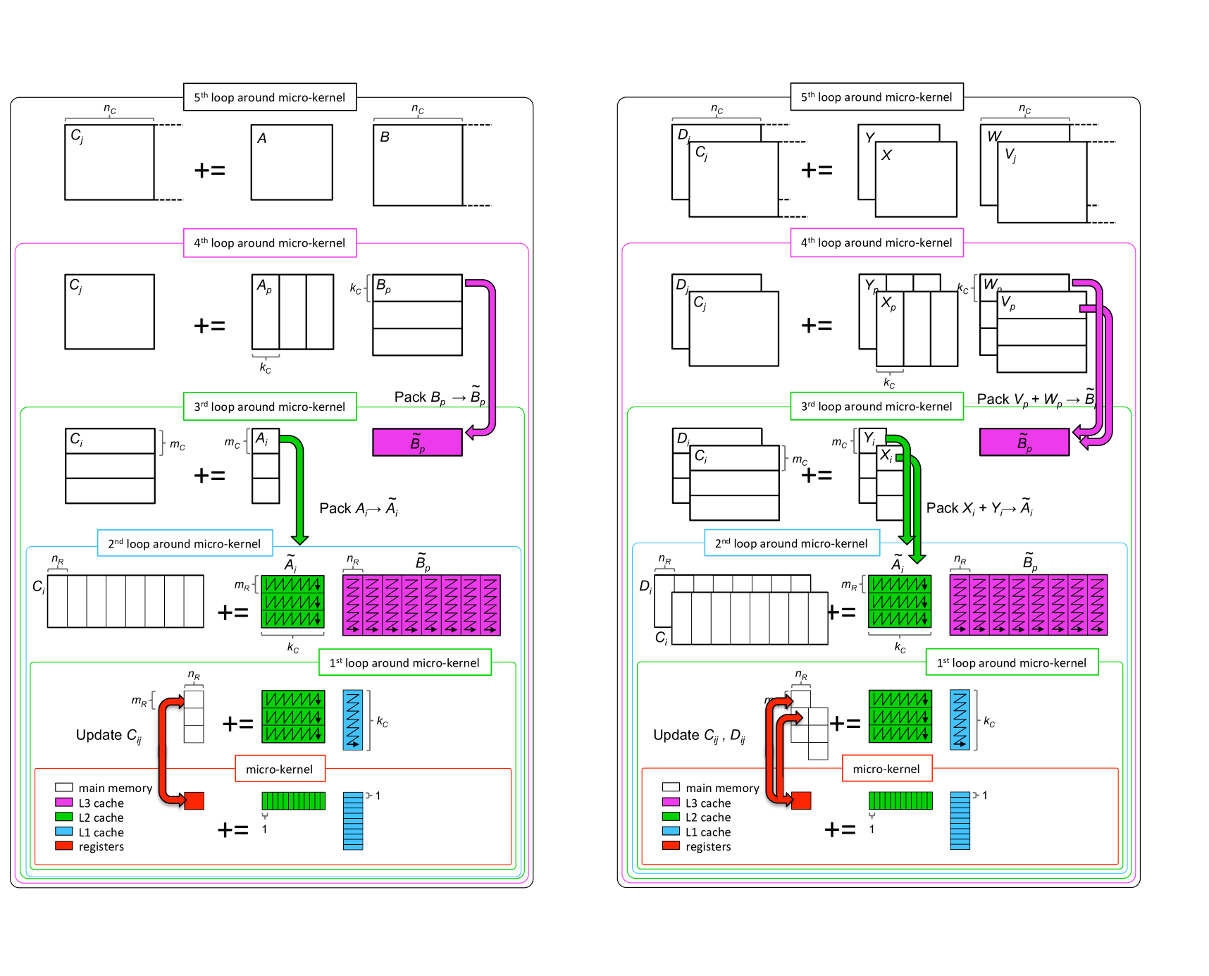
Key to high performance implementations of gemm is the partitioning of operands in order to (near-)optimally reuse data in the various levels of memory. Figure 1(left) illustrates how BLIS implements the GotoBLAS [6] approach. Block sizes are chosen so that submatrices fit in the various caches while relate to submatrices in registers that contribute to . These parameters can be analytically determined [7]. To improve data locality, row panels that fit in the L3 cache are “packed” into contiguous memory, yielding . For similar reasons, blocks that fit in the L2 cache are packed into buffer .
2.2 High-performance implementations of Strassen
If one partitions the three operands into quadrants,
| (1) |
then it can be shown that the operations
| (2) |
compute , but with seven (sub)matrix multiplications, reducing the cost by a factor of (ignoring a lower order number of extra additions). If all matrices are square and of size , classical Strassen exploits this recursively, reducing the cost for gemm to .
Only a few levels of the recursion are exploited in practice because the cost of extra additions and extra memory movements quickly offsets the reduction in floating point operations. Also, Strassen is known to become more numerically unstable particularly when more than two levels of recursion are employed [8, 9, 10].
In [2], captured in Figure 1(right), it was noted that the additions of the submatrices of and can be incorporated into the packing into buffers and , avoiding extra memory movements. In addition, once a submatrix that contributes to is computed in the registers, it can be directly added to the appropriate parts of multiple submatrices of , thus avoiding the need for temporary matrices , again avoiding extra memory movements. As demonstrated in [2], this makes the method practical for smaller matrices and matrices of special shape (especially rank-k updates, where is relatively small).
3 Fast Matrix Multiplication Algorithms
We now present the basic idea that underlies families of FMM algorithms and how to generalize one-level formula for multi-level FMM utilizing Kronecker products and recursive block storage indexing.
3.1 One-level fast matrix multiplication algorithms
In [1], the theory of tensor contractions is used to find a large number of FMM algorithms. In this subsection, we use the output (the resulting algorithms) of their approach.
Generalizing the partitioning for Strassen, consider , where , , and are , , and matrices, respectively. [1] defines a algorithm by partitioning
Note that , , and are the submatrices of , and , with a single index in the row major order. Then, is computed by,
for ,
| (3) |
where () is a matrix multiplication that can be done recursively, , , and are entries of a matrix , a matrix , and a matrix , respectively. Therefore, the classical matrix multiplication which needs submatrix multiplications can be completed with submatrix multiplications. The set of coefficients that determine the algorithm is denoted as .
For example, assuming that , , and are all even, one-level Strassen has partition dimensions and, given the partitioning in (1) and computations in (2),
| (4) |
specifies for one-level Strassen.
| Ref. | Speedup () | |||||||
| Theory | Practical #1 | Practical #2 | ||||||
| Ours | [1] | Ours | [1] | |||||
| [11] | ||||||||
| [1] | ||||||||
| [1] | ||||||||
| [10] | ||||||||
| [10] | ||||||||
| [10] | ||||||||
| [10] | ||||||||
| [10] | ||||||||
| [10] | ||||||||
| [12] | ||||||||
| [12] | ||||||||
| [1] | ||||||||
| [12] | ||||||||
| [12] | ||||||||
| [12] | ||||||||
| [10] | ||||||||
| [1] | ||||||||
| [10] | ||||||||
| [10] | ||||||||
| [10] | ||||||||
| [10] | ||||||||
| [10] | ||||||||
| [12] | ||||||||
3.2 Kronecker Product
If and are and matrices with entries denoted by and , respectively, then the Kronecker product [14] is the matrix given by
Thus, entry .
3.3 Recursive Block Indexing (Morton-like Ordering)
An example of recursive block storage indexing (Morton-like ordering) [15] is given in Figure 3. In this example, undergoes three levels of recursive splitting, and each submatrix of is indexed in row major form. By indexing , , and in this manner, data locality is maintained when operations are performed on their respective submatrices.
3.4 Representing two-level FMM with the Kronecker Product
In [3], it is shown that multi-level Strassen can be represented as Kronecker product. In this paper, we extend this insight to multi-level FMM, where each level can use a different choice of .
Assume each submatrix of , , and is partitioned with another level of FMM algorithm with the coefficients , and , , are the submatrices of , and , with a single index in two-level recursive block storage indexing. Then it can be verified that is computed by,
for ,
where represents Kronecker Product. Note that , , and are , , matrices, respectively.
The set of coefficients of a two-level and FMM algorithm can be denoted as .
For example, the two-level Strassen is represented by the coefficients where are the one-level Strassen coefficients given in (4).
3.5 Additional levels of FMM
Comparing one-level and two-level FMM, the same skeleton pattern emerges. The formula for defining -level FMM is given by,
for ,
| (5) |
The set of coefficients of an -level () FMM algorithm can be denoted as .
4 Implementation and Analysis
The last section shows that families of one-level FMM algorithms can be specified by and . It also shows how the Kronecker product can be used to generate multi-level FMM algorithms that are iterative rather than recursive. In this section, we discuss a code generator that takes as input and and as output generates implementations that build upon the primitives that combine taking linear combinations of matrices with the packing routines and/or micro-kernels that underlie BLIS. The code generator also provides a model of cost for each implementation that can then be used to choose the best FMM for a matrix of given size and shape. This code generator can thus generate code for arbitrary levels of FMM that can use different FMM choices at each level. In this way, we have generated and compared more than 200 FMM algorithms.
4.1 Code generation
Our code generator generates various implementations of FMM, based on the coefficient representation , levels of recursion, and packing routine/micro-kernel incorporation specifications.
There are two stages for our code generator: generating the skeleton framework, and generating the typical operations given in (3).
Generating the skeleton framework
During this stage, the code generator
-
•
Computes the Kronecker Product of the coefficient matrices in each level to get the new coefficients .
-
•
Generates the matrix partition code by conceptual recursive block storage indexing with partition dimensions for each level.
-
•
For the general cases where one or more dimensions are not multiples of corresponding , , , it generates dynamic peeling [16] code to handle the remaining “fringes” after invoking FMM, which requires no additional memory.
Generating the typical operations
To generate the code for the typical operations in (3), the code generator
-
•
Generates packing routines (written in C), that sum a list of submatrices of integrated into the packing routine, yielding , and similarly sum a list of submatrices of integrated into the packing routine, yielding , extending what is illustrated in Figure 1.
-
•
Assembles a specialized micro-kernel comprised of a hand-coded gemm kernel and automatically generated updates to multiple submatrices of .
Further variations
In [2], a number of variations on the theme illustrated in Figure 1 (right) are discussed:
-
•
Naive FMM: A classical implementation with temporary buffers for storing the sum of , , and the intermediate matrix product .
-
•
AB FMM: The packing routines incorporate the summation of submatrices of , into the packing of buffers and but explicit temporary buffers for matrices are used.
-
•
ABC FMM: AB FMM, but with a specialized micro-kernel that incorporates addition of to multiple submatrices of .
Incorporating the generation of these variations into the code generator yields over 200 FMM implementations.
4.2 Performance model
| Time (in sec.) of one arithmetic (floating point), | |
| operation, reciprocal of theoretical peak GFLOPS. | |
| (Bandwidth) Amortized time (in sec.) of 8 Bytes | |
| contigous data movement from DRAM to cache. | |
| Total execution time (in sec.). | |
| Time for arithmetic operations (in sec. ). | |
| Time for memory operations (in sec. ). | |
| for submatrix multiplications. | |
| , , | for extra submatrix additions. |
| , | for reading submatrices in packing routines (Fig. 1). |
| , | for writing submatrices in packing routines (Fig. 1). |
| for reading and writing submatrices in micro-kernel | |
| (Fig. 1). | |
| , , | for reading or writing submatrices, related to the |
| temporary buffer as part of Naive FMM and AB FMM. | |
| non-zero entry number in matrix or vector . |
| \raisebox{-0.9pt}{1}⃝ | |
|---|---|
| \raisebox{-0.9pt}{2}⃝ | |
| \raisebox{-0.9pt}{3}⃝ | |
| \raisebox{-0.9pt}{4}⃝ |
| type | gemm | -level | ||
| - | ||||
| - | - | |||
| - | - | |||
| - | - | |||
| r | ||||
| w | ||||
| r | ||||
| w | ||||
| r/w | ||||
| r/w | ||||
| r/w | ||||
| r/w |
| gemm | -level | |||
|---|---|---|---|---|
| ABC | AB | Naive | ||
| 1 | ||||
| - | ||||
| - | ||||
| - | ||||
| 1 | ||||
| - | - | - | - | |
| - | - | - | - | |
| 1 | ||||
| - | - | - | ||
| - | - | - | ||
| - | - | |||
In [2], a performance model was given to estimate the execution time for the one-level/two-level ABC, AB, and Naive variations of Strassen. In this subsection, we generalize that performance model to predict the execution time for the various FMM implementations generated by our code generator. Theoretical estimation helps us better understand the computation and memory footprint of different FMM implementations, and allows us to avoid exhaustive empirical search when searching for the best implementation for different problem sizes and shapes. Most importantly, our code generator can embed our performance model to guide the selection of a FMM implementation as a function of problem size and shape, with the input and specifications on each level . These performance models are themselves automatically generated.
Assumption
We have similar architecture assumptions as in [2]. Basically we assume that the architecture has two layers of modern memory hierarchy: fast caches and relatively slow main memory (DRAM). For read operations, the latency for accessing cache can be ignored, while the latency for accessing the main memory is counted; For write operations, we assume a lazy write-back policy such that the time for writing into fast caches can be hidden. Based on these assumptions, the memory operations for gemm and various implementations of FMM are decomposed into three parts:
Notation
Notation is summarized in Figure 4.
The total execution time, , is dominated by arithmetic time and memory time (\raisebox{-0.9pt}{2}⃝ in Figure 5).
Arithmetic operations
is decomposed into submatrix multiplications () and submatrix additions (, , ) (\raisebox{-0.9pt}{3}⃝ in Figure 5). has a coefficient 2 because under the hood the matrix additions are cast into FMA operations. The corresponding coefficients are tabulated in Figure 5. For instance, = for -level FMM, because computing in (5) involves = submatrix additions. Note that denotes the th column of .
Memory operations
is a function of the submatrix sizes {, , }, and the block sizes {, , } in Figure 1(right), because the memory operation can repeat multiple times according to which loop they reside in. is broken down into several components, as shown in \raisebox{-0.9pt}{4}⃝ in Figure 5. Each memory operation term is characterized in Figure 5 by its read/write type and the amount of memory in units of 64-bit double precision elements. Note that , are omitted in \raisebox{-0.9pt}{4}⃝ because of the assumption of lazy write-back policy with fast caches. Due to the software prefetching effects, has an additional parameter , which denotes the prefetching efficiency. is adapted to match gemm performance. Note that this is a ceiling function proportional to , because rank-k updates for accumulating submatrices of recur times in 4th loop in Figure 1. The corresponding coefficients are tabulated in Figure 5. For example, for Naive FMM and AB FMM, computing in (5) involves 2 read and 1 write related to temporary buffer in slow memory. Therefore, = .
4.3 Discussion
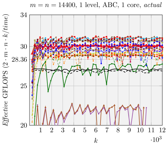
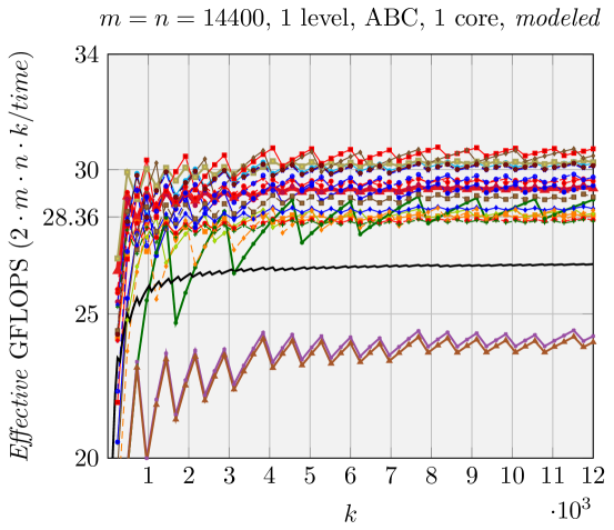
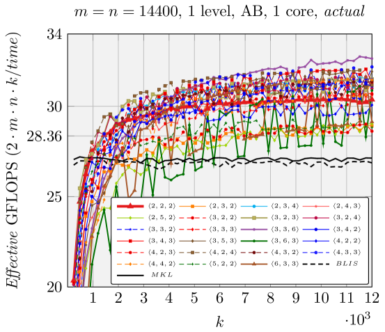
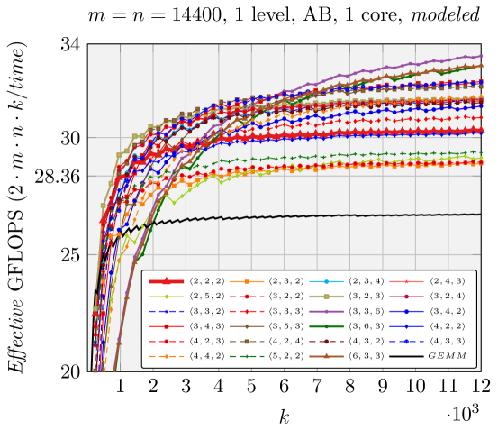
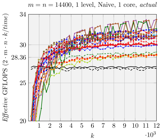
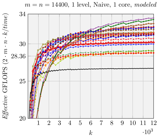
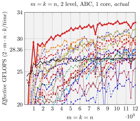
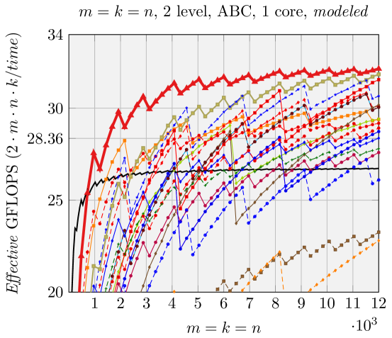
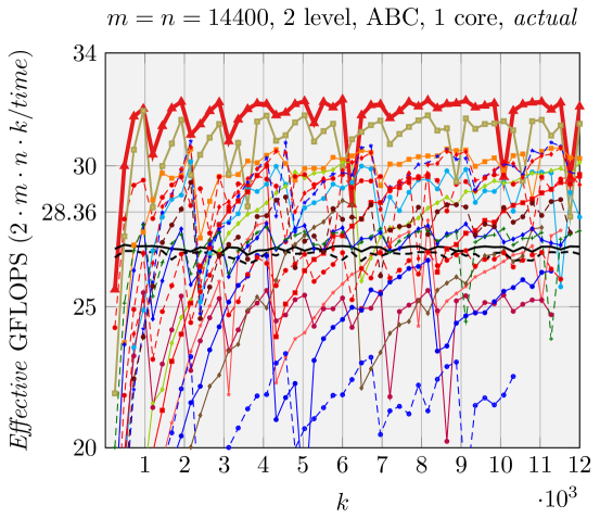
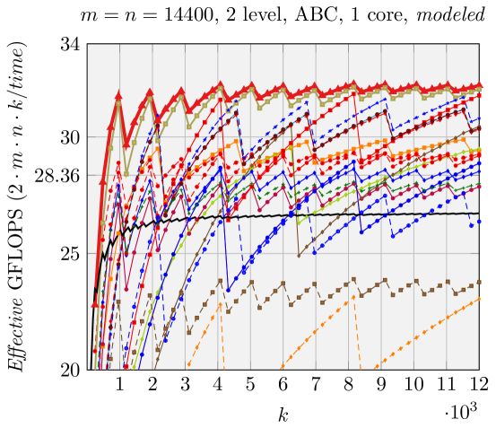
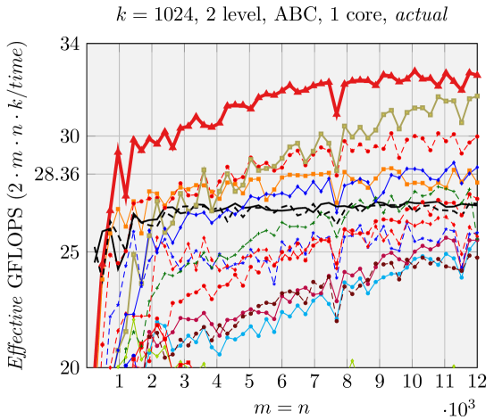
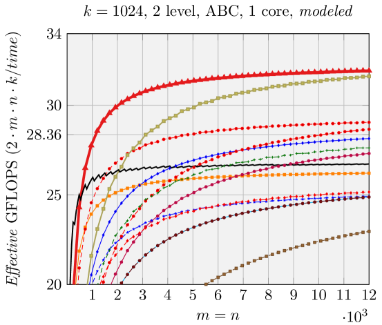
We can make estimations about the run time performance of the various FMM implementations generated by our code generator, based on the analysis shown in Figure 5. We use Effective GFLOPS (defined in \raisebox{-0.9pt}{1}⃝ in Figure 5) as the metric to compare the performance of these various FMM implementations, similar to [1, 17, 18]. The architecture-dependent parameters for the model are given in Section 5. We demonstrate the performance of two representative groups of experiments in Figures 6 and 7.
-
•
Contrary to what was observed in [2], Naive FMM may perform better than ABC FMM and AB FMM for relatively large problem size. For example, in Figure 6, (with the maximum theoretical speedup among all FMMs we test, Figure 2) has better Naive FMM performance than ABC FMM and AB FMM. This is because the total number of times for packing in is very large (, ). This magnifies the overhead for packing with AB FMM/ABC FMM.
-
•
Contrary to what was observed in [1], for rank-k updates (middle column, right column, Figure 7), still performs the best with ABC FMM implementations ([1] observe some other shapes, e.g. , tend to have higher performance). This is because their implementations are similar to Naive FMM, with the overhead for forming the matrices explicitly.
- •
- •
4.4 Apply performance model to code generator
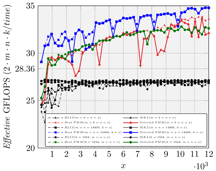
For actual performance, even the best implementation has some unexpected drops, due to the “fringes” which are caused by the problem sizes not being divisible by partition dimesions , , . This is not captured by our performance model. Therefore, given the specific problem size and shape, we choose the best two implementations predicted by our performance model as the top two candidate implementations, and then measure the performance in practice to pick the best one.
In Figure 8 we show the performance results on single core by selecting the generated FMM implementation with the guide of performance model, when ; , varies; and , vary.
Overall this experiment shows that the performance model is accurate enough in terms of relative performance between various FMM implementations to guide the choice of a FMM implementation, with the problem sizes and shapes as the inputs. That will reduce the potential overhead of exhaustive empirical search.
5 Performance Experiments
We present performance evaluations for various generated FMM implementations.
5.1 Implementation and architecture information
The FMM implementations generated by our code generator are written in C, utilizing SSE2 and AVX assembly, compiled with the Intel C compiler version 15.0.3 with optimization flag -O3 -mavx.
We compare against our generated dgemm (based on the packing routines and micro-kernel borrowed from BLIS, marked as BLIS in the performance figures) as well as Intel MKL’s dgemm [19] (marked as MKL in the performance figures).
We measure performance on a dual-socket (10 cores/socket) Intel Xeon E5-2680 v2 (Ivy Bridge) processor with 12.8 GB/core of memory (Peak Bandwidth: 59.7 GB/s with four channels) and a three-level cache: 32 KB L1 data cache, 256 KB L2 cache and 25.6 MB L3 cache. The stable CPU clockrate is 3.54 GHz when a single core is utilized (28.32 GFLOPS peak, marked in the graphs) and 3.10 GHz when ten cores are in use (24.8 GLOPS/core peak). To set thread affinity and to ensure the computation and the memory allocation all reside on the same socket, we use KMP_AFFINITY=compact.
The blocking parameters, , , , and , are consistent with parameters used for the standard BLIS dgemm implementation for this architecture. This makes the size of the packing buffer 192 KB and 8192 KB, which then fit the L2 cache and L3 cache, respectively.
5.2 Benefit of hybrid partitions
First, we demonstrate the benefit of using different FMM algorithms for each level.
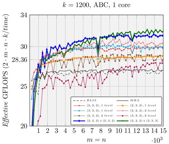
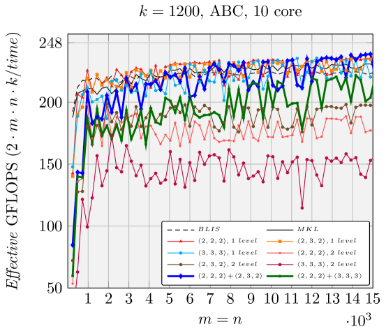
We report the performance of different combinations of one-level/two-level , , and in Figure 9, when is fixed to 1200 and vary. As suggested and illustrated in Section 4.3, ABC FMM performs best for rank-k updates, which is why we only show the ABC FMM performance.
Overall the hybrid partitions + and + achieve the best performance. This is because 1200 is close to , meaning that the hybrid partitions of 2 and 3 on the dimension are more favorable. This is consistent with what the performance model predicts. Performance benefits are less for 10 cores due to bandwidth limitations, although performance of hybrid partitions still beats two-level homogeneous partitions.
This experiment shows the benefit of hybrid partitions, facilitated by the Kronecker product representation.
5.3 Sequential and parallel performance
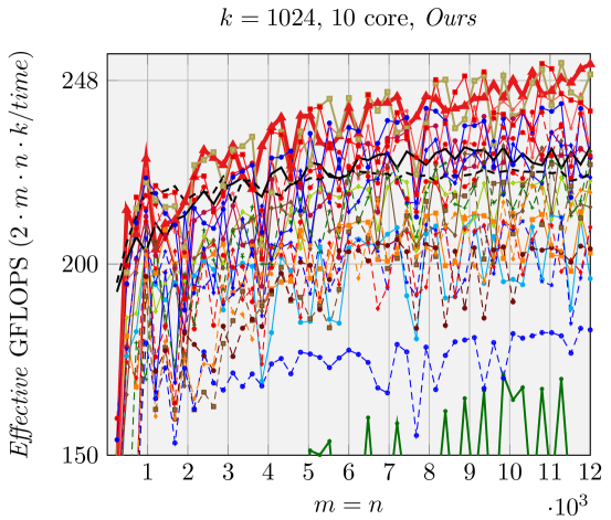
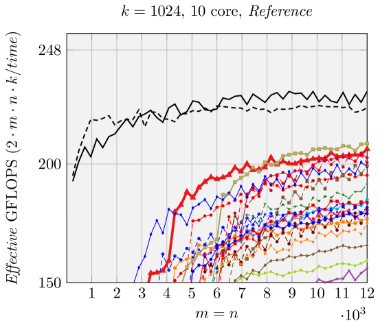
Results when using a single core are presented in Figures 2, 6, and 7. Our generated ABC FMM implementation outperforms AB FMM/Naive FMM and reference implementations from [1] for rank-k updates (when is small). For very large square matrices, our generated AB FMM or Naive FMM can achieve competitive performance with reference implementations [1] that is linked with Intel MKL. These experiments support the validity of our model.
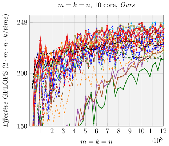
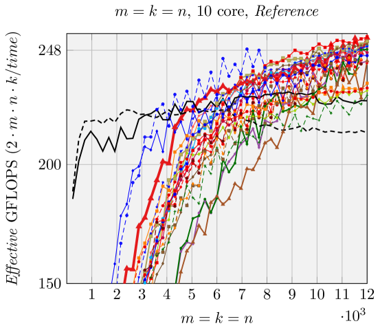
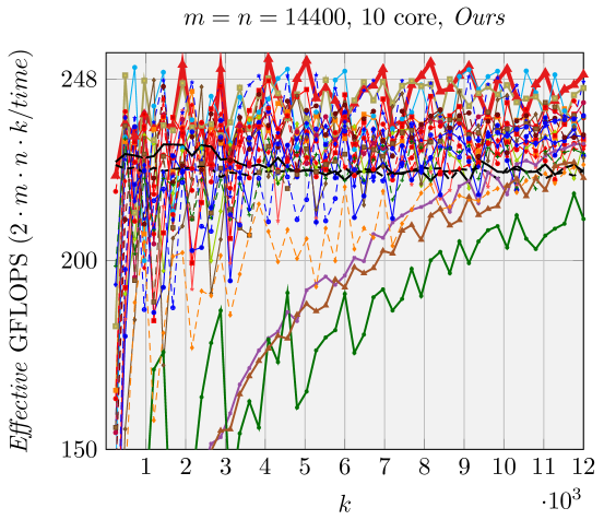
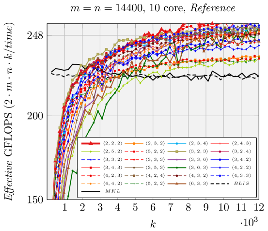
Figure 10 reports performance results for ten cores within the same socket. Memory bandwidth contention impacts the performance of various FMM when using many cores. Nonetheless we still observe the speedup of FMM over gemm. For smaller matrices and special shapes such as rank-k updates, our generated implementations achieve better performance than reference implementations [1].
6 Conclusion
We have discussed a code generator framework that can automatically implement families of FMM algorithms for Strassen-like fast matrix multiplication algorithms. This code generator expresses the composition of multi-level FMM algorithms as Kronecker products. It incorporates the matrix summations that must be performed for FMM into the inherent packing and micro-kernel operations inside gemm, avoiding extra workspace requirement and reducing the overhead of memory movement. Importantly, it generates an accurate performance model to guide the selection of a FMM implementation as a function of problem size and shape, facilitating the creation of poly-algorithms that select the best algorithm for a problem size. Comparing with state-of-the-art results, we observe a significant performance improvement for smaller matrices and special matrix multiplication shapes such as rank-k updates, without the need for exhaustive empirical search.
There are a number of avenues for future work:
- •
-
•
Finding the new FMM algorithms by searching the coefficient matrix is an NP-hard problem [22]. It may be possible to prune branches with the performance model as the cost function during the search process.
-
•
In [2], it is shown that Intel Xeon Phi coprocessor (KNC) can benefit from ABC variation of Strassen. It may be possible to get performance benefit by porting our code generator to generate variations of FMM implementations for many-core architecture such as second-generation Intel Xeon Phi coprocessor (KNL).
Additional information
Additional information regarding BLIS and related projects can be found at
http://shpc.ices.utexas.edu
Acknowledgments
This work was sponsored in part by the National Science Foundation under grant number ACI-1550493, by Intel Corporation through an Intel Parallel Computing Center grant, and by a gift from Qualcomm. Access to the Maverick supercomputers administered by TACC is gratefully acknowledged. Jianyu Huang was supported by a summer fellowship from Graduate School of UT Austin. DAM is an Arnold O. Beckman Postdoctoral Fellow. We thank the rest of the SHPC team (http://shpc.ices.utexas.edu) for their supports.
Any opinions, findings, and conclusions or recommendations expressed in this material are those of the author(s) and do not necessarily reflect the views of the National Science Foundation.
References
- [1] A. R. Benson and G. Ballard, “A framework for practical parallel fast matrix multiplication,” in Proceedings of the 20th ACM SIGPLAN Symposium on Principles and Practice of Parallel Programming, ser. PPoPP 2015. New York, NY, USA: ACM, 2015, pp. 42–53.
- [2] J. Huang, T. M. Smith, G. M. Henry, and R. A. van de Geijn, “Strassen’s algorithm reloaded,” in Proceedings of the International Conference for High Performance Computing, Networking, Storage and Analysis, ser. SC ’16. New York, NY, USA: ACM, 2016.
- [3] C.-H. Huang, J. R. Johnson, and R. W. Johnson, “A tensor product formulation of Strassen’s matrix multiplication algorithm,” Applied Mathematics Letters, vol. 3, no. 3, pp. 67–71, 1990.
- [4] J. Li, A. Skjellum, and R. D. Falgout, “A poly-algorithm for parallel dense matrix multiplication on two-dimensional process grid topologies,” Concurrency: Practice and Experience, vol. 9, no. 5, pp. 345–389, May 1997.
- [5] F. G. Van Zee and R. A. van de Geijn, “BLIS: A framework for rapidly instantiating BLAS functionality,” ACM Trans. Math. Soft., vol. 41, no. 3, pp. 14:1–14:33, June 2015. [Online]. Available: http://doi.acm.org/10.1145/2764454
- [6] K. Goto and R. A. van de Geijn, “Anatomy of a high-performance matrix multiplication,” ACM Trans. Math. Soft., vol. 34, no. 3, p. 12, May 2008, article 12, 25 pages.
- [7] Tze Meng Low, F. D. Igual, T. M. Smith, and E. S. Quintana-Ortí, “Analytical modeling is enough for high performance blis,” ACM Transactions on Mathematical Software, in review.
- [8] N. J. Higham, Accuracy and Stability of Numerical Algorithms, 2nd ed. Philadelphia, PA, USA: SIAM, 2002.
- [9] J. Demmel, I. Dumitriu, O. Holtz, and R. Kleinberg, “Fast matrix multiplication is stable,” Numerische Mathematik, vol. 106, no. 2, pp. 199–224, 2007.
- [10] G. Ballard, A. R. Benson, A. Druinsky, B. Lipshitz, and O. Schwartz, “Improving the numerical stability of fast matrix multiplication,” SIAM Journal on Matrix Analysis and Applications, vol. 37, no. 4, pp. 1382–1418, 2016.
- [11] V. Strassen, “Gaussian elimination is not optimal,” Numer. Math., vol. 13, pp. 354–356, 1969.
- [12] A. V. Smirnov, “The bilinear complexity and practical algorithms for matrix multiplication,” Computational Mathematics and Mathematical Physics, vol. 53, no. 12, pp. 1781–1795, 2013. [Online]. Available: http://dx.doi.org/10.1134/S0965542513120129
- [13] D. Bini, M. Capovani, F. Romani, and G. Lotti, “O () complexity for approximate matrix multiplication,” Information processing letters, vol. 8, no. 5, pp. 234–235, 1979.
- [14] A. Graham, “Kronecker products and matrix calculus: With applications.” JOHN WILEY & SONS, INC., 605 THIRD AVE., NEW YORK, NY 10158, 1982, 130, 1982.
- [15] E. Elmroth, F. Gustavson, I. Jonsson, and B. Kågström, “Recursive blocked algorithms and hybrid data structures for dense matrix library software,” SIAM review, vol. 46, no. 1, pp. 3–45, 2004.
- [16] M. Thottethodi, S. Chatterjee, and A. R. Lebeck, “Tuning Strassen’s matrix multiplication for memory efficiency,” in Proceedings of the 1998 ACM/IEEE Conference on Supercomputing, ser. SC ’98. Washington, DC, USA: IEEE Computer Society, 1998, pp. 1–14. [Online]. Available: http://dl.acm.org/citation.cfm?id=509058.509094
- [17] B. Grayson and R. van de Geijn, “A high performance parallel Strassen implementation,” Parallel Processing Letters, vol. 6, no. 1, pp. 3–12, 1996.
- [18] B. Lipshitz, G. Ballard, J. Demmel, and O. Schwartz, “Communication-avoiding parallel Strassen: Implementation and performance,” in Proceedings of the International Conference on High Performance Computing, Networking, Storage and Analysis, ser. SC ’12. Los Alamitos, CA, USA: IEEE Computer Society Press, 2012, pp. 101:1–101:11.
- [19] “Intel Math Kernel Library,” https://software.intel.com/en-us/intel-mkl.
- [20] T. M. Smith, R. A. van de Geijn, M. Smelyanskiy, J. R. Hammond, and F. G. Van Zee, “Anatomy of high-performance many-threaded matrix multiplication,” in 28th IEEE International Parallel and Distributed Processing Symposium (IPDPS 2014), 2014.
- [21] P. D’Alberto, M. Bodrato, and A. Nicolau, “Exploiting parallelism in matrix-computation kernels for symmetric multiprocessor systems: Matrix-multiplication and matrix-addition algorithm optimizations by software pipelining and threads allocation,” ACM Trans. Math. Softw., vol. 38, no. 1, pp. 2:1–2:30, December 2011. [Online]. Available: http://doi.acm.org/10.1145/2049662.2049664
- [22] D. E. Knuth, The Art of Computer Programming, Volume 2 (3rd Ed.): Seminumerical Algorithms. Boston, MA, USA: Addison-Wesley Longman Publishing Co., Inc., 1997.