Generation of Talbot-like fields

In recent years there has been much interest in the propagation of light in free space where it has been shown that light not only propagates in straight lines but there are beams that also bend while propagating [1, 2, 3, 4, 5, 6, 7, 8, 9, 10, 11, 12, 13, 14, 15].

On the other hand, Montgomery [16] has given the necessary and sufficient conditions in order that a given field at $z=0$, replicates itself without the aid of lenses or other optical accessories, i.e., for the Talbot effect to take place.

In this contribution, by using eigenfunctions of the perpendicular Laplacian in polar coordinates, we show that an integral of diffraction may be written which we use to propagate some fields, namely Bessel and superposition of Airy beams, both divided by the square root of the radial coordinate. We also show that particular series of Bessel beams with integer or fractional order, reproduce themselves during propagation, ı.e., giving rise to the Talbot effect.

If we consider the field at z = 0 given in the form

$$E(r,\theta,0)=\frac{\hbox{e}^{i\theta/2}}{\sqrt{r}}\int_{-\infty}^{\infty}\mathcal{E}(\alpha)\hbox{e}^{ir\alpha}d\alpha\;,$$

(5)

it is easy to see that we may write an integral of diffraction of the form

$$E(r,\theta,z)=\frac{\hbox{e}^{i\theta/2}}{\sqrt{r}}\int_{-\infty}^{\infty}\hbox{e}^{{\color[rgb]{0,0,0}\definecolor[named]{pgfstrokecolor}{rgb}{0,0,0}\pgfsys@color@gray@stroke{0}\pgfsys@color@gray@fill{0}-}i\frac{z}{2}\alpha^{2}}\mathcal{E}(\alpha)\hbox{e}^{ir\alpha}d\alpha,$$

(6)

where we have applied the property that a function of (the operator) $\nabla_{\perp}^{2}$ applied to the eigenfunction is simply the function of the eigenvalue times the eigenfunction, i.e.,

$\displaystyle F(\nabla_{\perp}^{2})\frac{\hbox{e}^{i\alpha r}}{\sqrt{r}}\hbox{e}^{\pm i\frac{\theta}{2}}=F(-\alpha^{2})\frac{\hbox{e}^{i\alpha r}}{\sqrt{r}}\hbox{e}^{\pm i\frac{\theta}{2}}.$

(7)

We consider the following field at $z=0$

$$E(r,\theta,z=0)=\frac{J_{n}(ar)}{\sqrt{r}}\hbox{e}^{i\frac{\theta}{2}},\qquad n\geq 1,$$

(8)

where $J_{n}(x)$ is a Bessel function of order $n$ and the case $n=0$ is not considered because of its singularity. We write the Bessel function in terms of its integral representation

$$E(r,\theta,z=0)=\frac{1}{2\pi}\int_{-\pi}^{\pi}\frac{\hbox{e}^{iar\sin u}}{\sqrt{r}}\hbox{e}^{i\frac{\theta}{2}}\hbox{e}^{-inu}du,$$

(9)

such that, by applying the property described by Eq. (7), we obtain

$$E(r,\theta,z)=\frac{\hbox{e}^{i\frac{\theta}{2}}}{2\pi\sqrt{r}}\int_{-\pi}^{\pi}\hbox{e}^{{\color[rgb]{0,0,0}\definecolor[named]{pgfstrokecolor}{rgb}{0,0,0}\pgfsys@color@gray@stroke{0}\pgfsys@color@gray@fill{0}-}i\frac{a^{2}z}{2}\sin^{2}u}\hbox{e}^{iar\sin u-inu}du.$$

(10)

It is not difficult to show that the integral above is a so-called Generalized Bessel function. For this, we rewrite it as

$$E(r,\theta,z)=\frac{\hbox{e}^{{\color[rgb]{0,0,0}\definecolor[named]{pgfstrokecolor}{rgb}{0,0,0}\pgfsys@color@gray@stroke{0}\pgfsys@color@gray@fill{0}-}i\frac{a^{2}z}{\color[rgb]{0,0,0}\definecolor[named]{pgfstrokecolor}{rgb}{0,0,0}\pgfsys@color@gray@stroke{0}\pgfsys@color@gray@fill{0}4}}\hbox{e}^{i\frac{\theta}{2}}}{2\pi\sqrt{r}}\int_{-\pi}^{\pi}\hbox{e}^{i\frac{a^{2}z}{4}\cos 2u}\hbox{e}^{iar\sin u-inu}du.$$

(11)

We define $Z=a^{2}z/{\color[rgb]{0,0,0}\definecolor[named]{pgfstrokecolor}{rgb}{0,0,0}\pgfsys@color@gray@stroke{0}\pgfsys@color@gray@fill{0}4}$ and use a Taylor series for the cosine term argument exponential, yielding

$$E(r,\theta,z)=\frac{\hbox{e}^{{\color[rgb]{0,0,0}\definecolor[named]{pgfstrokecolor}{rgb}{0,0,0}\pgfsys@color@gray@stroke{0}\pgfsys@color@gray@fill{0}-}iZ}\hbox{e}^{i\frac{\theta}{2}}}{2\pi\sqrt{r}}\sum_{m=0}^{\infty}\frac{(iZ)^{m}}{2^{m}m!}\int_{-\pi}^{\pi}(\hbox{e}^{2iu}+\hbox{e}^{-2iu})^{m}\hbox{e}^{iar\sin u-inu}du,$$

(12)

and developing the binomial inside the integral we obtain

	$\displaystyle E(r,\theta,z)$	$\displaystyle=$	$\displaystyle\frac{\hbox{e}^{{\color[rgb]{0,0,0}\definecolor[named]{pgfstrokecolor}{rgb}{0,0,0}\pgfsys@color@gray@stroke{0}\pgfsys@color@gray@fill{0}-}iZ}\hbox{e}^{i\frac{\theta}{2}}}{2\pi\sqrt{r}}\sum_{m=0}^{\infty}\frac{(iZ)^{m}}{2^{m}m!}\times$		(16)
			$\displaystyle\sum_{k=0}^{m}\left(\begin{array}[]{c}m\\ k\end{array}\right)\int_{-\pi}^{\pi}\hbox{e}^{2iu(m-2k)}\hbox{e}^{iar\sin u-inu}du.$

We extend the second sum to infinity as we would only add zeros to the sum and exchange the order of the sums

	$\displaystyle E(r,\theta,z)$	$\displaystyle=$	$\displaystyle\frac{\hbox{e}^{{\color[rgb]{0,0,0}\definecolor[named]{pgfstrokecolor}{rgb}{0,0,0}\pgfsys@color@gray@stroke{0}\pgfsys@color@gray@fill{0}-}iZ}\hbox{e}^{i\frac{\theta}{2}}}{2\pi\sqrt{r}}\sum_{k=0}^{\infty}\sum_{m=0}^{\infty}\frac{(iZ)^{m}}{2^{m}k!(m-k)!}\times$		(17)
			$\displaystyle\int_{-\pi}^{\pi}\hbox{e}^{2iu(m-2k)}\hbox{e}^{iar\sin u-inu}du,$

and start the sum that runs on $m$ at $m=k$ (as for $m<k$ the terms added are zero)

	$\displaystyle E(r,\theta,z)$	$\displaystyle=$	$\displaystyle\frac{\hbox{e}^{{\color[rgb]{0,0,0}\definecolor[named]{pgfstrokecolor}{rgb}{0,0,0}\pgfsys@color@gray@stroke{0}\pgfsys@color@gray@fill{0}-}iZ}\hbox{e}^{i\frac{\theta}{2}}}{2\pi\sqrt{r}}\sum_{k=0}^{\infty}\sum_{m=k}^{\infty}\frac{(iZ)^{m}}{2^{m}k!(m-k)!}\times$		(18)
			$\displaystyle\int_{-\pi}^{\pi}\hbox{e}^{2iu(m-2k)}\hbox{e}^{iar\sin u-inu}du.$

By letting $j=m-k$ we obtain

	$\displaystyle E(r,\theta,z)$	$\displaystyle=$	$\displaystyle\frac{\hbox{e}^{{\color[rgb]{0,0,0}\definecolor[named]{pgfstrokecolor}{rgb}{0,0,0}\pgfsys@color@gray@stroke{0}\pgfsys@color@gray@fill{0}-}iZ}\hbox{e}^{i\frac{\theta}{2}}}{2\pi\sqrt{r}}\sum_{k=0}^{\infty}\sum_{j=0}^{\infty}\frac{(iZ)^{j+k}}{2^{j+k}k!j!}$		(19)
		$\displaystyle\times$	$\displaystyle\int_{-\pi}^{\pi}\hbox{e}^{2iu(j-k)}\hbox{e}^{iar\sin u-inu}du,$

that, by using the integral representation of Bessel functions, gives

$$E(r,\theta,z)=\frac{\hbox{e}^{{\color[rgb]{0,0,0}\definecolor[named]{pgfstrokecolor}{rgb}{0,0,0}\pgfsys@color@gray@stroke{0}\pgfsys@color@gray@fill{0}-}iZ}\hbox{e}^{i\frac{\theta}{2}}}{\sqrt{r}}\sum_{k=0}^{\infty}\sum_{j=0}^{\infty}\frac{(iZ)^{j+k}}{2^{j+k}k!j!}J_{n+2(k-j)}(ar).$$

(20)

By letting $s=k-j$ we obtain

$$E(r,\theta,z)=\frac{\hbox{e}^{{\color[rgb]{0,0,0}\definecolor[named]{pgfstrokecolor}{rgb}{0,0,0}\pgfsys@color@gray@stroke{0}\pgfsys@color@gray@fill{0}-}iZ}\hbox{e}^{i\frac{\theta}{2}}}{\sqrt{r}}\sum_{s=-\infty}^{\infty}J_{n+2s}(ar)\sum_{j=0}^{\infty}\frac{(iZ)^{2j+s}}{2^{2j+s}(j+s)!j!},$$

(21)

where we have extended the sum on $s$ to minus infinity as we simply add zeros.

This finally gives a sum of two Bessel functions of different order

$$E(r,\theta,z)=\frac{\hbox{e}^{{\color[rgb]{0,0,0}\definecolor[named]{pgfstrokecolor}{rgb}{0,0,0}\pgfsys@color@gray@stroke{0}\pgfsys@color@gray@fill{0}-}iZ}\hbox{e}^{i\frac{\theta}{2}}}{\sqrt{r}}\sum_{s=-\infty}^{\infty}i^{s}J_{n+2s}(ar)J_{s}({\color[rgb]{0,0,0}\definecolor[named]{pgfstrokecolor}{rgb}{0,0,0}\pgfsys@color@gray@stroke{0}\pgfsys@color@gray@fill{0}Z}),$$

(22)

that may be added to give the so-called Generalized Bessel functions studied by Dattoli et al. [17, 18] and Eichelkraut [19]. By using that Bessel generalized functions, given by the expression $\mathcal{J}_{n}(r,z;g)=\sum_{s=-\infty}^{\infty}g^{s}J_{n-2s}(r)J_{s}(z)$, we write the propagated field as

$$E(r,\theta,z)=\frac{\hbox{e}^{{\color[rgb]{0,0,0}\definecolor[named]{pgfstrokecolor}{rgb}{0,0,0}\pgfsys@color@gray@stroke{0}\pgfsys@color@gray@fill{0}-}iZ}\hbox{e}^{i\frac{\theta}{2}}}{\sqrt{r}}\mathcal{J}_{n}(ar,{\color[rgb]{0,0,0}\definecolor[named]{pgfstrokecolor}{rgb}{0,0,0}\pgfsys@color@gray@stroke{0}\pgfsys@color@gray@fill{0}Z};i).$$

(23)

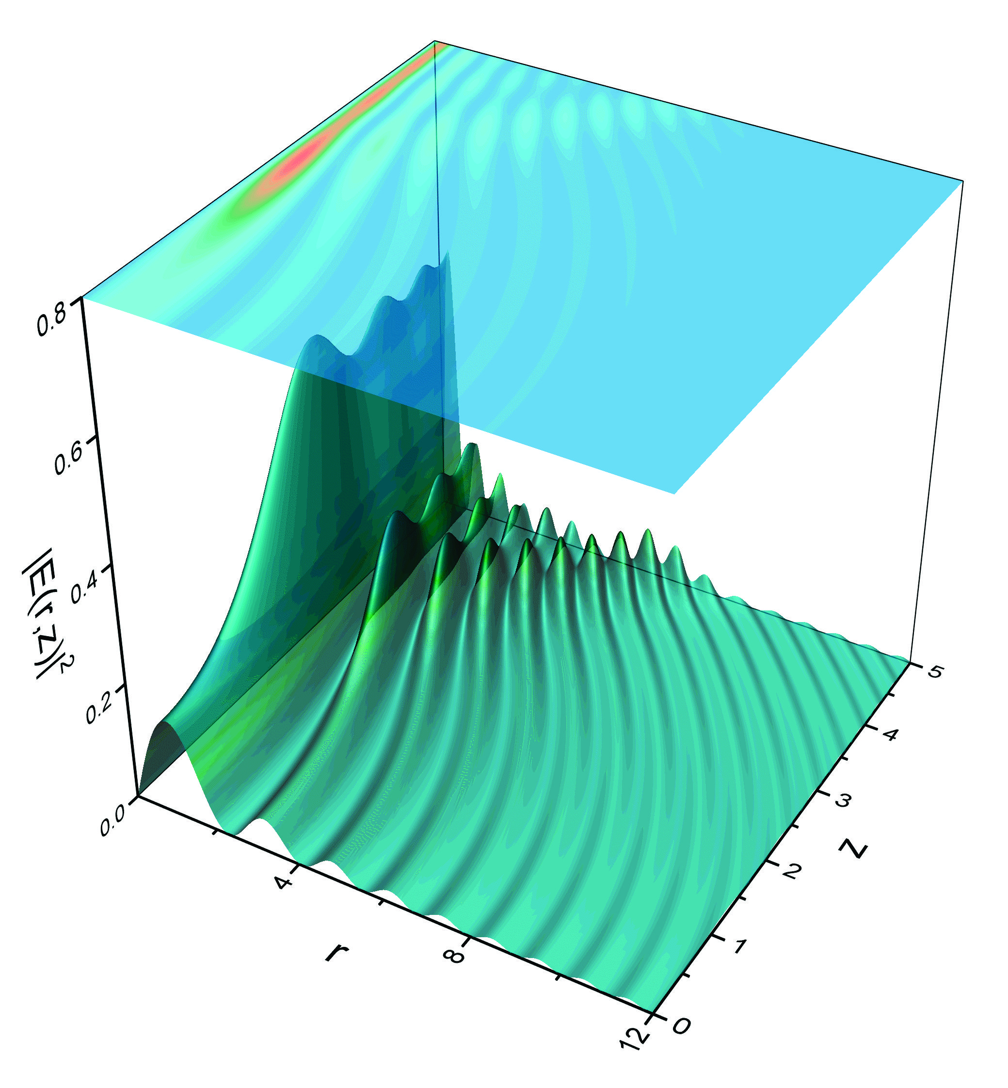
In Fig. 1 we plot the field intensity for an initial Bessel function of order $n=1$ as a function of the propagation distance and the radial coordinate. It may be observed that there is an energy redistribution from the central rings towards the outer rings as the field propagates, nevertheless, an overall intensity decrease also exists.

We now study the propagation of a superposition of Airy beams [2, 6] whose distribution at $z=0$ is given by

	$\displaystyle E(r,\theta,z=0)$	$\displaystyle=$	$\displaystyle\frac{\hbox{e}^{i\frac{\theta}{2}}}{2\pi\sqrt{r}}\left[\int_{-\infty}^{\infty}\hbox{e}^{i\left(\frac{t^{3}}{3}+rt\right)}\right.dt$		(24)
		$\displaystyle-$	$\displaystyle\left.\int_{-\infty}^{\infty}\hbox{e}^{i\left(\frac{t^{3}}{3}-rt\right)}dt\right],$

where we have written the Airy function in its integral representation. By applying the integral of diffraction given by Eq. (5) we obtain

	$\displaystyle E(r,\theta,z)$	$\displaystyle=$	$\displaystyle\frac{\hbox{e}^{i\frac{\theta}{2}}}{2\pi\sqrt{r}}\left[\int_{-\infty}^{\infty}\hbox{e}^{i\left(\frac{t^{3}}{3}+rt\right)}\hbox{e}^{{\color[rgb]{0,0,0}\definecolor[named]{pgfstrokecolor}{rgb}{0,0,0}\pgfsys@color@gray@stroke{0}\pgfsys@color@gray@fill{0}-}i\frac{zt^{2}}{2}}dt\right.$		(25)
		$\displaystyle-$	$\displaystyle\left.\int_{-\infty}^{\infty}\hbox{e}^{i\left(\frac{t^{3}}{3}-rt\right)}\hbox{e}^{{\color[rgb]{0,0,0}\definecolor[named]{pgfstrokecolor}{rgb}{0,0,0}\pgfsys@color@gray@stroke{0}\pgfsys@color@gray@fill{0}-}i\frac{zt^{2}}{2}}dt\right].$

By changing variables in the integrals above, we may rewrite them as

	$\displaystyle E(r,\theta,z)$	$\displaystyle=$	$\displaystyle\frac{\hbox{e}^{{\color[rgb]{0,0,0}\definecolor[named]{pgfstrokecolor}{rgb}{0,0,0}\pgfsys@color@gray@stroke{0}\pgfsys@color@gray@fill{0}-}i\frac{z^{3}}{12}}\hbox{e}^{i\frac{\theta}{2}}}{2\pi\sqrt{r}}\left[\hbox{e}^{i\frac{rz}{2}}\int_{-\infty}^{\infty}\hbox{e}^{i\left(\frac{t^{3}}{3}+\left[r{\color[rgb]{0,0,0}\definecolor[named]{pgfstrokecolor}{rgb}{0,0,0}\pgfsys@color@gray@stroke{0}\pgfsys@color@gray@fill{0}-}\frac{z^{2}}{4}\right]t\right)}dt\right.$		(26)
		$\displaystyle-$	$\displaystyle\left.\hbox{e}^{{\color[rgb]{0,0,0}\definecolor[named]{pgfstrokecolor}{rgb}{0,0,0}\pgfsys@color@gray@stroke{0}\pgfsys@color@gray@fill{0}-}i\frac{rz}{2}}\int_{-\infty}^{\infty}\hbox{e}^{i\left(\frac{t^{3}}{3}-\left[r{\color[rgb]{0,0,0}\definecolor[named]{pgfstrokecolor}{rgb}{0,0,0}\pgfsys@color@gray@stroke{0}\pgfsys@color@gray@fill{0}+}\frac{z^{2}}{4}\right]t\right)}dt\right],$

that finally yields the superposition of Airy functions

	$\displaystyle E(r,\theta,z)$	$\displaystyle=$	$\displaystyle\frac{\hbox{e}^{{\color[rgb]{0,0,0}\definecolor[named]{pgfstrokecolor}{rgb}{0,0,0}\pgfsys@color@gray@stroke{0}\pgfsys@color@gray@fill{0}-}i\frac{z^{3}}{12}}\hbox{e}^{i\frac{\theta}{2}}}{\sqrt{r}}\left(\hbox{e}^{{\color[rgb]{0,0,0}\definecolor[named]{pgfstrokecolor}{rgb}{0,0,0}\pgfsys@color@gray@stroke{0}\pgfsys@color@gray@fill{0}+}i\frac{rz}{2}}\hbox{Ai}\left[r{\color[rgb]{0,0,0}\definecolor[named]{pgfstrokecolor}{rgb}{0,0,0}\pgfsys@color@gray@stroke{0}\pgfsys@color@gray@fill{0}-}\frac{z^{2}}{4}\right]\right.$		(27)
		$\displaystyle-$	$\displaystyle\left.\hbox{e}^{{\color[rgb]{0,0,0}\definecolor[named]{pgfstrokecolor}{rgb}{0,0,0}\pgfsys@color@gray@stroke{0}\pgfsys@color@gray@fill{0}-}i\frac{rz}{2}}\hbox{Ai}\left[-r{\color[rgb]{0,0,0}\definecolor[named]{pgfstrokecolor}{rgb}{0,0,0}\pgfsys@color@gray@stroke{0}\pgfsys@color@gray@fill{0}-}\frac{z^{2}}{4}\right]\right).$

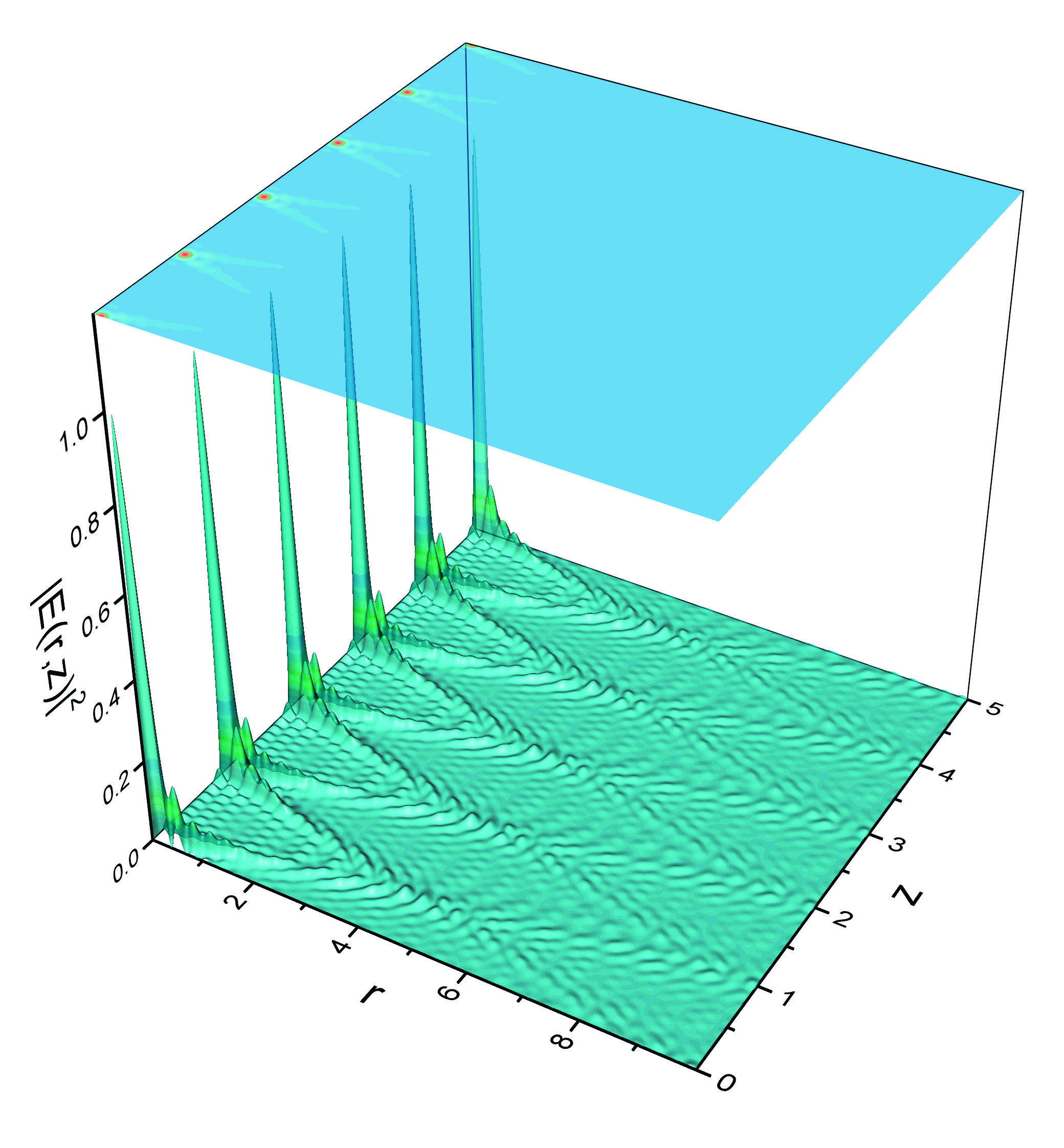
We plot the propagated field intensity in Fig. 2 where it may be observed abrupt focusing that may be attributed to the superposition of the Airy functions. There is one Airy function whose main contribution would be in the negative part of the axis, and would bend towards the right. However, as $r$ is always positive, it does not have enough weight to produce an effect. On the other hand, the Airy function whose main contribution is on the positive part, dominates the propagation and bends towards the left. Although there is no medium, the focusing may be explained by the fact that the Airy function produces an effective index of refraction (the so-called Bohm potential in quantum mechanics) [20, 21] that gives rise to such behaviour.

We can superimpose the eigenfunctions described by Eq. (4), with the same eigenvalue to find another eigenfunction, a beam of the form $\frac{\sin{br}}{\sqrt{r}}$, which takes us to a Bessel function of order one half

$$E(r,\theta,z=0)=J_{\frac{1}{2}}(br)\hbox{e}^{i\frac{\theta}{2}},$$

(28)

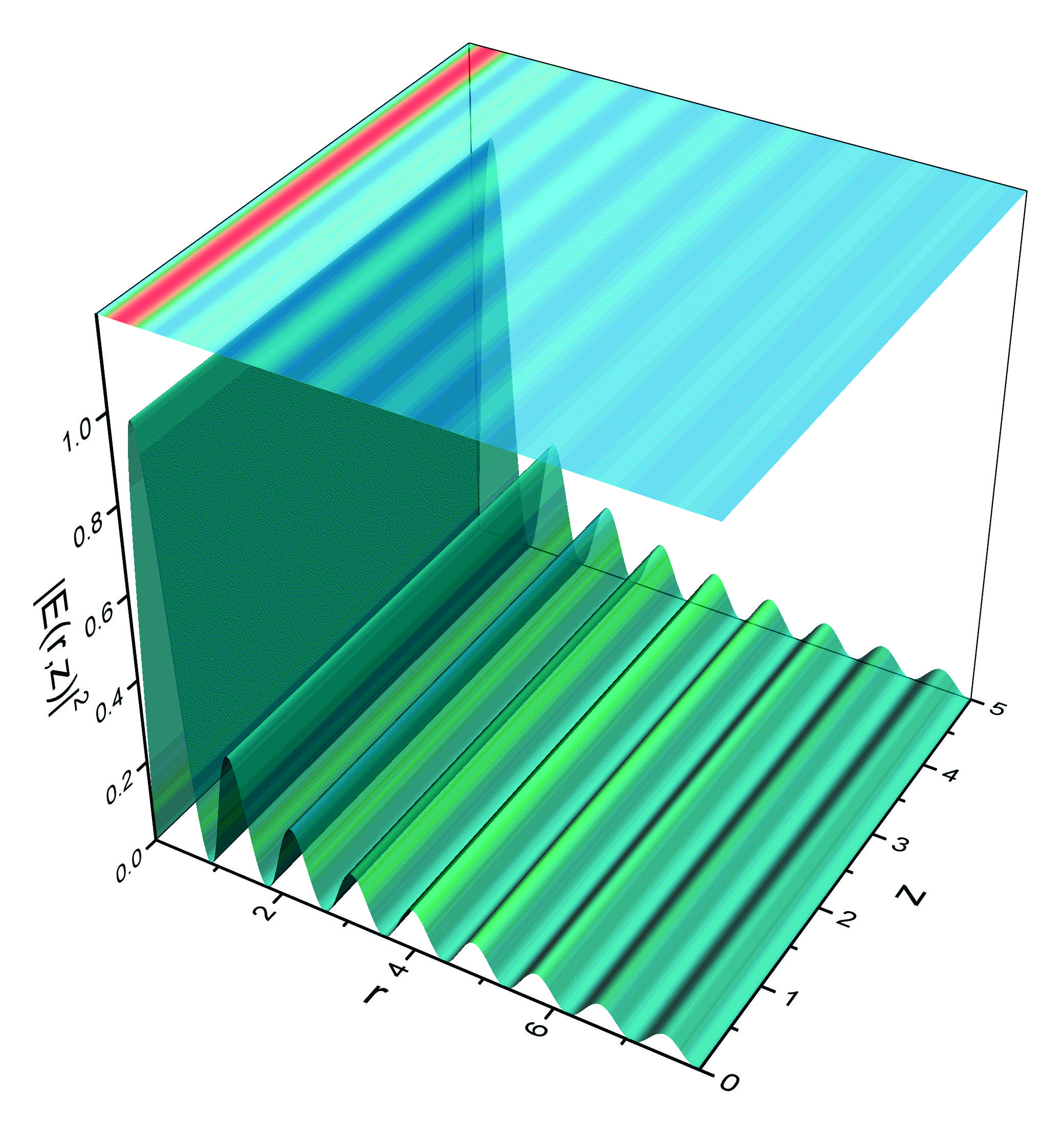
that is indeed, a diffraction-free beam and we plot it in Fig. 3.

We then may show that, a proper superposition of them

$$E(r,\theta,z=0)=\hbox{e}^{i\frac{\theta}{2}}\sum_{k=1}^{N}c_{k}J_{\frac{1}{2}}\left(\sqrt{2^{k+1}\pi}r\right),$$

(29)

propagates as

$$E(r,\theta,z)=\hbox{e}^{i\frac{\theta}{2}}\sum_{k=1}^{N}e^{-i2^{k}z\pi}c_{k}J_{\frac{1}{2}}\left(\sqrt{2^{k+1}\pi}r\right),$$

(30)

that recovers periodically the field at $z=0$,

	$\displaystyle E(r,\theta,z=n)$	$\displaystyle=$	$\displaystyle\hbox{e}^{i\frac{\theta}{2}}\sum_{k=1}^{N}e^{-i2^{k}n\pi}c_{k}J_{\frac{1}{2}}\left(\sqrt{2^{k+1}\pi}r\right)$		(31)
		$\displaystyle=$	$\displaystyle E(r,\theta,z=0).$

We plot in Fig. 4 the field propagated for $c_{k}=1$ and $N=10$, where it may be seen clearly this effect.

We have shown that by properly writing a field at $z=0$ we may propagate it by using an integral of diffraction that we introduced in this manuscript. We have shown how to propagate Bessel and a superposition of Airy beams (over the square root of the radial coordinate) and have shown that a series of Bessel functions that may have integer or fractional order and with proper parameters reproduces itself during propagation, therefore producing the Talbot effect. We have shown self focusing of the superposition of Airy beams that may be explained by the existence of an effective index of refraction related to the Bohm potential.

References

• [1] M. V. Berry and N. L. Balazs, “Nonspreading wave packets,” Am. J. Phys. 47, 264–267 (1979).
• [2] G. A. Siviloglou, J. Broky, A. Dogariu, and D. N. Christodoulides, “Observation of accelerating airy beams,” Phys. Rev. Lett. 99, 213901 (2007).
• [3] C.-Y. Hwang, D. Choi, K.-Y. Kim, and B. Lee, “Dual airy beam,” Opt. Express 18, 23504–23516 (2010).
• [4] S. Chávez-Cerda, U. Ruiz, V. Arrizón, and H. M. Moya-Cessa, “Generation of airy solitary-like wave beams by acceleration control in inhomogeneous media,” Opt. Express 19, 16448–16454 (2011).
• [5] S. Yan, B. Yao, M. Lei, D. Dan, Y. Yang, and P. Gao, “Virtual source for an airy beam,” Opt. Lett. 37, 4774–4776 (2012).
• [6] P. Vaveliuk, A. Lencina, J. A. Rodrigo, and O. M. Matos, “Symmetric airy beams,” Opt. Lett. 39, 2370–2373 (2014).
• [7] R. Jáuregui and P. Quinto-Su, “On the general properties of symmetric incomplete airy beams,” J. Opt. Soc. Am. A 31, 2484–2488 (2014).
• [8] P. Vaveliuk, A. Lencina, J. A. Rodrigo, and O. M. Matos, “Intensitysymmetric airy beams,” J. Opt. Soc. Am. A 32, 443–446 (2015).
• [9] Y. Kaganovsky and E. Heyman, “Wave analysis of airy beams,” Opt. Express 18, 8440–8452 (2010).
• [10] D. G. Papazoglou, V. Y. Fedorov, and S. Tzortzakis, “Janus waves,” Opt. Lett. 41, 4656–4659 (2016).
• [11] A. Torre, “Propagating airy wavelet-related patterns,” J. Opt. 17, 075604 (2015).
• [12] P. Aleahmad, H. Moya-Cessa, I. Kaminer, M. Segev, and D. N. Christodoulides, “Dynamics of accelerating bessel solutions of maxwell’s equations,” J.Opt. Soc. Am. A 33, 2047–2052 (2016).
• [13] D. Weisman, S. Fu, M. Gonçalves, L. Shemer, J. Zhou, W. P. Schleich, and A. Arie, “Diffractive focusing of waves in time and in space,” Phys. Rev. Lett. 118, 154301 (2017).
• [14] D. Mansour and D. G. Papazoglou, “Tailoring the focal region of abruptly autofocusing and autodefocusing ring-airy beams,” OSA Continuum 1, 104–115 (2018).
• [15] G. G. Rozenman, M. Zimmermann, M. A. Efremov, W. P. Schleich, L. Shemer, and A. Arie, “Amplitude and phase of wave packets in a linear potential,” Phys. Rev. Lett. 122, 124302 (2019).
• [16] W. D. Montgomery, “Self-imaging objects of infinite aperture,” J.Opt. Soc. Am. 57, 772–778 (1967).
• [17] G. Dattoli, L. Giannessi, M. Richetta, and A. Torre, “Miscellaneous results on infinite series of bessel functions,” Il Nuovo Cimento 103B, 149–159 (1989).
• [18] G. Dattoli, A. Torre, S. Lorenzutta, G. M. S., and C. Chiccoli, “Theory of generalized bessel functions.-ii,” Il Nuovo Cimento 101, 21–51 (1991).
• [19] T. Eichelkraut, C. Vetter, A. Perez-Leija, H. Moya-Cessa, D. N. Christodoulides, and A. Szameit, “Coherent random walks in free space,” Optica 1, 268–271 (2014).
• [20] F. A.Asenjo, S. A. Hojman, H. M. Moya-Cessa, and F. Soto-Eguibar, “Propagation of light in linear and quadratic grin media: The bohm potential,” Opt. Commun. 490, 126947 (2021).
• [21] Sergio A. Hojman, Felipe A. Asenjo, and H.M. Moya-Cessa and F. Soto-Eguibar, “Bohm potential is real and its effects are measurable,” Optik 232, 166341 (2021).
• [22] I. Gradshteyn and I. Ryzhik, Table of integrals, series, and products (Academic Press, Inc., San Diego, 1980).
• [23] J. J. Durnin, J. J. Miceli and J. H. Eberly, “Diffraction-free beams,” Phys. Rev. Lett. 58, 1499–1501 (1987).