GenTree: Using Decision Trees to Learn Interactions for Configurable Software
Abstract
Modern software systems are increasingly designed to be highly configurable, which increases flexibility but can make programs harder to develop, test, and analyze, e.g., how configuration options are set to reach certain locations, what characterizes the configuration space of an interesting or buggy program behavior? We introduce GenTree, a new dynamic analysis that automatically learns a program’s interactions—logical formulae that describe how configuration option settings map to code coverage. GenTree uses an iterative refinement approach that runs the program under a small sample of configurations to obtain coverage data; uses a custom classifying algorithm on these data to build decision trees representing interaction candidates; and then analyzes the trees to generate new configurations to further refine the trees and interactions in the next iteration. Our experiments on 17 configurable systems spanning 4 languages show that GenTree efficiently finds precise interactions using a tiny fraction of the configuration space.
I Introduction
Modern software systems are increasingly designed to be configurable. This has many benefits, but also significantly complicates tasks such as testing, debugging, and analysis due to the number of configurations that can be exponentially large—in the worst case, every combination of option settings can lead to a distinct behavior. This software configuration space explosion presents real challenges to software developers. It makes testing and debugging more difficult as faults are often visible under only specific combinations of configuration options. It also causes a challenge to static analyses because configurable systems often have huge configuration spaces and use libraries and native code that are difficult to reason about.
Existing works on highly-configurable systems [1, 2, 3, 4] showed that we can automatically find interactions to concisely describe the configuration space of the system. These works focus on program coverage (but can be generalized to arbitrary program behaviors) and define an interaction for a location as a logically weakest formula over configuration options such that any configuration satisfying that formula would cover that location. These works showed that interactions are useful to understand the configurations of the system, e.g., determine what configuration settings cover a given location; determine what locations a given interaction covers; find important options, and compute a minimal set of configurations to achieve certain coverage; etc. In the software production line community, feature interactions and presence conditions (§VII) are similar to interactions and has led to many automated configuration-aware testing techniques to debug functional (e.g., bug triggers, memory leaks) and non-functional (e.g., performance anomalies, power consumption) behaviors. Interactions also help reverse engineering and impact analysis [5, 6], and even in the bioinformatics systems for aligning and analyzing DNA sequences [7].
These interaction techniques are promising, but have several limitations. The symbolic execution work in [1] does not scale to large systems, even when being restricted to configuration options with a small number of values (e.g., boolean); needs user-supplied models (mocks) to represent libraries, frameworks, and native code; and is language-specific (C programs). iTree [2, 3] uses decision trees to generate configurations to maximize coverage, but achieves very few and imprecise interactions. Both of these works only focus on interactions that can be represented as purely conjunctive formulae.
The iGen interaction work [4] adopts the iterative refinement approach often used to find program preconditions and invariants (e.g., [8, 9, 10, 11]). This approach learns candidate invariants from program execution traces and uses an oracle (e.g., a static checker) to check the candidates. When the candidate invariants are incorrect, the oracle returns counterexample traces that the dynamic inference engine can use to infer more accurate invariants. iGen adapts this iterative algorithm to finding interactions, but avoids static checking, which has limitations similar to symbolic execution as mentioned above. Instead, iGen modifies certain parts of the candidate interaction to generate new configurations and run them to test the candidate. Configurations that “break” the interaction are counterexamples used to improve that interaction in the next iteration. However, to effectively test interactions and generate counterexample configurations, iGen is restricted to learning interactions under specific forms (purely conjunctive, purely disjunctive, and specific mixtures of the two) and thus cannot capture complex interactions in real-world systems (§VI).
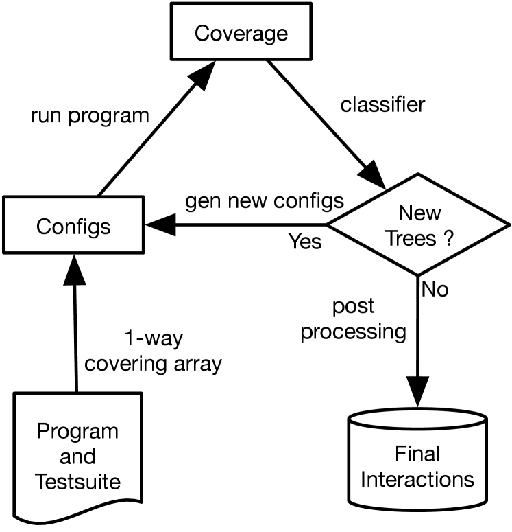
In this paper, we introduce GenTree, a new dynamic interaction inference technique inspired by the iterative invariant refinement algorithm and iGen. Figure 2 gives an overview of GenTree. First, GenTree creates an initial set of configurations and runs the program to obtain (location) coverage. Then for each covered location , GenTree builds a decision tree, which represents a candidate interaction, from the configurations that do and do not cover .
Because GenTree works with just a sample of all configurations, the decision trees representing candidate interactions may be imprecise. To refine these trees, GenTree analyzes them to generate new configurations. In the next iteration, these configurations may provide the necessary data to invalidate the current trees (i.e., counterexamples) and build more precise trees, which correspond to better interactions. This process continues until we obtain no new coverage or trees for several consecutive iterations, at which point GenTree returns the final set of interactions.
The design of GenTree helps mitigate several limitations of existing works. By using dynamic analysis, GenTree is language agnostic and supports complex programs (e.g., those using third party libraries) that might be difficult for static analyses. By considering only small configuration samples, GenTree is efficient and scales well to large programs. By integrating with iterative refinement, GenTree generates small sets of useful configurations to gradually improve its results. By using decision trees, GenTree supports expressive interactions representing arbitrary boolean formulae and allows for generating effective counterexample configurations. Finally, by using a classification algorithm customized for interactions, GenTree can build trees from small data samples to represent accurate interactions.
We evaluated GenTree on 17 programs in C, Python, Perl, and OCaml having configuration spaces containing to configurations. We found that interaction results from GenTree are precise, i.e., similar to what GenTree would produce if it inferred interactions from all possible configurations. We also found that GenTree scales well to programs with many options because it only explores a small fraction of the large configuration spaces. We examined GenTree’s results and found that they confirmed several observations made by prior work (e.g., conjunctive interactions are common but disjunctive and mixed interactions are still important for coverage; and enabling options, which must be set in a certain way to cover most locations, are common). We also observed that complex interactions supported by GenTree but not from prior works cover a non-trivial number of locations and are critical to understand the program behaviors at these locations.
In summary, this paper makes the following contributions: (i) we introduce a new iterative refinement algorithm that uses decision trees to represent and refine program interactions; (ii) we present a decision tree classification algorithm optimized for interaction discovery; (iii) we implement these ideas in the GenTree tool and make it freely available; and (iv) we evaluate GenTree on programs written in various languages and analyze its results to find interesting configuration properties. GenTree and all benchmark data are available at [12].
II Illustration
We use the C program in Figure 2 to explain GenTree. This program has nine configuration options listed on the first line of the figure. The four options are boolean-valued, and the other five options, , range over the set . The configuration space of this program thus has possible configurations.
The code in Figure 2 includes print statements that mark nine locations –. At each location, we list the associated desired interaction. For example, is covered by any configuration in which is true, is 2, and either or is false. is covered by every configuration (i.e., having the interaction true), but is not covered by every configuration because the program returns when it reaches or .
Prior interaction inference approaches are not sufficient for this example. The works of Reisner et. al [1] and iTree [2, 3] only support conjunctions and therefore cannot generate the correct interactions for any locations except , , and . The iGen tool [4], which supports conjunctions, disjunctions, and a limited form of both conjunctions and disjunctions, also cannot generate the interactions for locations and .
Initial Configurations
Decision Trees
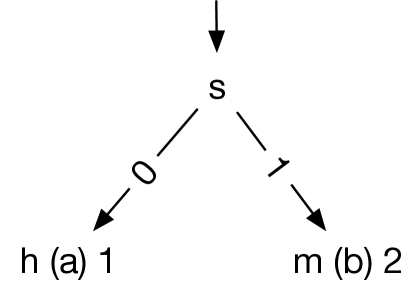
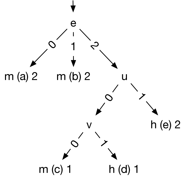
For each covered location , GenTree uses a classification algorithm called C5, developed specifically for this work, (§IV-B) to build a decision tree representing the interaction for . To build the tree for , C5 uses two sets of data: the hit sets consisting of configurations covering and the miss set consisting of configurations not covering . For example, for , GenTree builds the decision tree in Figure 5 from the hit sets and the miss set .
From the given configurations C5 determines that the coverage of just requires option being 0 (false). Thus, the interaction for , represented by the condition of the hit path (a) of the tree in Figure 5, is . This interaction is quite different than , the desired interaction for . However, even with only three initial configurations, the tree is partially correct because configurations having as true would miss and being false is part of the requirements for hitting .
New Configurations
GenTree now attempts to create new configurations to refine the tree representing the interaction for location . Observe that if a hit path is precise, then any configuration satisfying its condition would cover (similarly, any configuration satisfying the condition of a miss path would not cover ). Thus, we can validate a path by generating configurations satisfying its condition and checking their coverage. Configurations generated from a hit (or miss) path that do not (or do) cover are counterexample configurations, which show the imprecision of the path condition and help build a more precise tree in the next iteration.
In the running example, GenTree selects the condition of the hit path (a) of the tree shown in Figure 5 and generates four new configurations shown in Figure 5 with and 1-covering values for the other eight variables. If path (a) is precise, then these configurations would cover . However, only configuration covers . Thus, , which do not cover , are counterexamples showing that path (a) is imprecise and thus is not the correct interaction for .
Note that we could also generate new configurations using path (b), which represents the interaction for not covering . However, GenTree prefers path (a) because the classifier uses one configuration for path (a) and two for path (b), i.e., the condition for covering is only supported by one configuration and thus is likely more imprecise.
Next Iterations
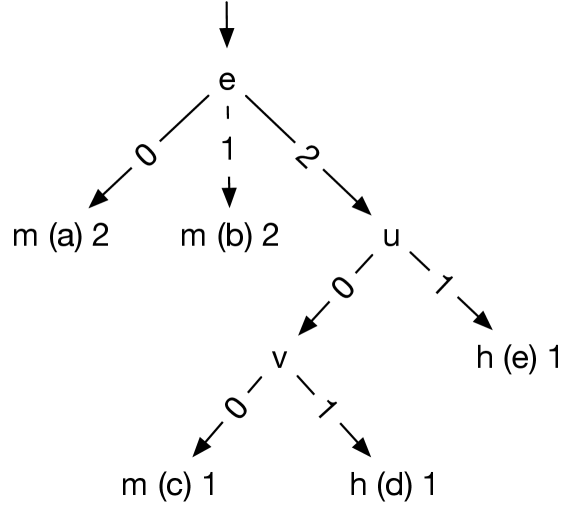
GenTree now repeats the process of building trees and generating new configurations. Continuing with our example on finding the interaction for , GenTree adds to the hit set and to the miss set and builds the new tree for in Figure 5. The combination of the hit paths (d) and (e) gives as the interaction for . This interaction contains options , which appear in the desired interaction .
To validate the new interaction for , GenTree generates new configurations from paths (c), (d), (e) of the tree in Figure 5, because they have the fewest number of supporting configurations. Figure 5 shows the nine new configurations.
Note that (c) is a miss path and thus are not counterexamples because they do not hit . Also, in an actual run, GenTree would select only one of these three paths and take two additional iterations to obtain these configurations. For illustration purposes, we combine these iterations and show the generated configurations all together.
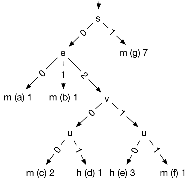
In the next iteration, using the new configurations and the previous ones, GenTree builds the decision tree in Figure 5 for . The interaction obtained from the two hit paths (d) and (e) is , which is equivalent to the desired one and thus would remain unchanged regardless of any additional configurations GenTree might create.
Finally, GenTree stops when it cannot generate new coverage or refine existing trees for several consecutive iterations. In a postprocessing step, GenTree combines the hit path conditions of the decision tree for each location into a logical formula representing the interaction for .
Complete Run
GenTree found the correct interactions for all locations in the running example within eight iterations and under a second. The table below shows the number of iterations and configurations used to find the interaction for each location. For example, the desired interaction for took 58 configurations and is discovered at iteration 4, and the interaction true of L0 was quickly discovered from the initial configurations.
| L0 | L1 | L2 | L3 | L4 | L5 | L6 | L7 | L8 | |
|---|---|---|---|---|---|---|---|---|---|
| Iter. Found | 1 | 2 | 6 | 1 | 2 | 5 | 3 | 3 | 4 |
| # Configs | 3 | 27 | 144 | 15 | 30 | 123 | 50 | 47 | 58 |
Overall, GenTree found all of these interactions by analyzing approximately 360 configurations (median over 11 runs) out of 3888 possible ones. The experiments in §VI show that GenTree analyzes an even smaller fraction of the possible configurations on programs with larger configuration spaces.
III Preliminaries
A configurable software consists of multiple configuration options, where each option plays a similar role as a global program variable, but often has a finite domain (e.g., boolean) and does not change during program execution. A configuration is a set of settings of the form , where is a configuration option and is a (valid) value of .
Interactions
An interaction for a location characterizes of the set of configurations covering . For example, we see from Figure 2 that any configuration satisfying (i.e., they have the settings and ) is guaranteed to cover L3. Although we focus on location coverage, interaction can be associated with more general program behaviors, e.g., we could use an interaction to characterize configurations triggering some undesirable behavior. To obtain coverage, we typically run the program using a configuration and a test suite, which is a set of fixed environment data or options to run the program on, e.g., the test suite for the Unix ls (listing) command might consist of directories to run ls on. In summary, we define program interactions as:
Definition III.1.
Given a program , a test suite , and a coverage criterion (e.g., some location or behavior ), an interaction for is a formula over the (initial settings of the) configuration options of such that (a) any configuration satisfying is guaranteed to cover under and (b) is the logically weakest such formula (i.e., if also describes configurations covering then ).
Decision Trees
We use a decision tree to represent the interaction for a location . A decision tree consists of a root, leaves, and internal (non-leaf) nodes. Each non-leaf node is labeled with a configuration option and has outgoing edges, which correspond to the possible values of the option. Each leaf is labeled with a hit or miss class, which represents the classification of that leaf. The path from the root to a leaf represents a condition leading to the classification of the leaf. This path condition is the conjunction of the settings collected along that path. The union (disjunction) of the hit conditions is the interaction for . Dually, the disjunction of the miss conditions is the condition for not covering . The length of a path is the number of edges in the path.
For illustration purposes, we annotate each leaf with a label , where is either the (h) hit or (m) miss class, is the path name (so that we can refer to the path), and is the number of supporting configurations used to classify this path. Intuitively, the more supporting configurations a path has, the higher confidence we have about its classification.
For example, the decision tree in Figure 5 for location consists of four internal nodes and seven leaves. The tree has five miss and two hit paths, e.g., path (d), which has length 4 and condition , is classified as a hit due to one configuration hitting ( in Figure 5), and (g) is a miss path with condition because seven configurations satisfying this condition miss . The interaction for is , the disjunction of the two hit conditions.
IV The GenTree Algorithm
Figure 1 shows the GenTree algorithm, which takes as input a program, a test suite, and an optional set of initial configurations, and returns a set of interactions for locations in the program that were covered. Initial configurations, e.g., default or factory-installed configurations, if available, are useful starting points because they often give high coverage.
GenTree starts by creating a set of configurations using a randomly generated 1-covering array and the initial configurations if they are available. GenTree then runs the program on configs using the test suite and obtain their coverage.
Next, GenTree enters a loop that iteratively builds a decision tree for each covered location (§IV-B) and generates new configurations from these trees (§IV-A) in order to refine them. GenTree has two modes: exploit and explore. It starts in exploit mode and refines incorrect trees in each iteration. When GenTree can no longer refine trees (e.g., it is stuck in some plateau), it switches to explore mode and generates random configurations, hoping that these could help improve the trees (and if so, GenTree switches back to exploit mode in the next iteration).
For each covered location , GenTree performs the following steps. First, we create hit and miss sets consisting of configurations hitting or missing , respectively. Second, if GenTree is in exploit mode, we build a decision tree for from the hit and miss sets of configurations if either is a new location (a tree for does not exist) or that the existing tree for is not correct (the test_tree function checks if the tree fails to classify some configurations). If both of these are not true (i.e., the existing tree for is correct), we continue to the next location. Otherwise, if GenTree is in explore mode, we continue to the next step. Third, we rank and select paths in the tree that are likely incorrect to refine them. If GenTree is in explore mode, we also select random paths. Finally, we generate new configurations using the selected paths and obtain their coverage. GenTree uses these configurations to validate and refine the decision tree for in the next iteration.
GenTree repeats these steps until existing trees remain the same and no new trees are generated (i.e., no new coverage) for several iterations. In the end, GenTree uses a postprocessing step to extract logical formulae from generated trees to represent program interactions.
IV-A Selecting Paths and Generating Configurations
Given a decision tree, GenTree ranks paths in the tree and generates new configurations from high-ranked ones. Intuitively, we use configurations generated from a path to validate that path condition, which represents an interaction. If these configurations do not violate the path condition, we gain confidence in the corresponding interaction. Otherwise, these configurations are counterexamples that are subsequently used to learn a new tree with more accurate paths.
Selecting Paths
To select paths to generate new configurations, GenTree favors those with fewer supporting configurations because such paths are likely inaccurate and thus generating counterexample configurations to “break” them is likely easier.
If there are multiple paths with a similar number of supporting configurations, we break ties by choosing the longest ones. Paths with few supporting configurations but involving many options are likely more fragile and inaccurate. If there are multiple paths with a similar length and number of supporting configurations, we pick one arbitrary.
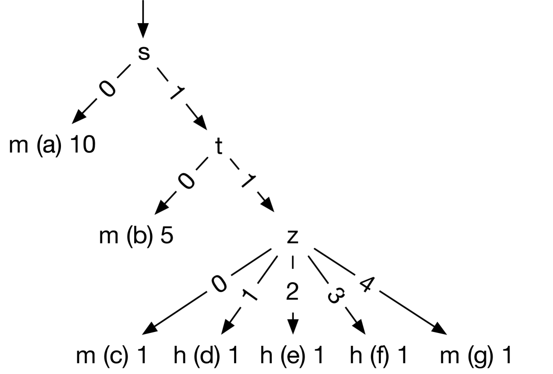
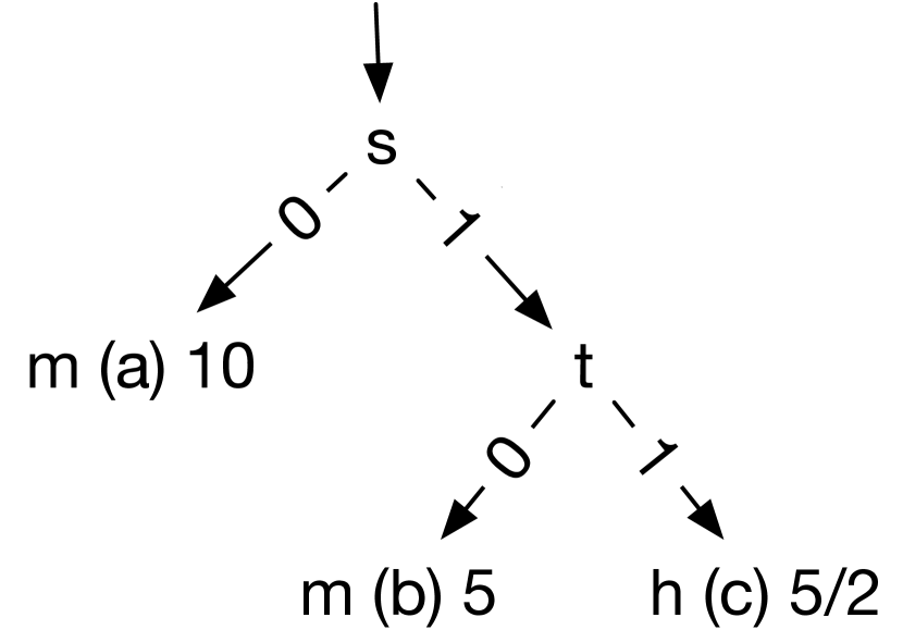
For example, paths (c) and (d) in the tree shown in Figure 6 have the highest rank because they each have just one supporting configuration. Paths (a), (b), and (e) have two configurations each, but path (e) is longer and thus ranked higher. The final ranking for this tree is then (c), (d), (e), (a), and (b).
Generating Configurations
From the highest-ranked path, GenTree generates 1-covering configurations that satisfy the path condition, i.e., these configurations have the same settings as those in the condition of that path. GenTree keeps generating new configurations this way for the next highest-ranked paths until it achieves up to a certain number of new configurations (currently configured to generate at least two new configurations).
Using high-ranked paths to generate configurations is a greedy approach, which might not always give useful configurations that help improve the tree. Thus, GenTree also selects random paths during the explore mode, i.e., when a tree remains unchanged in the previous iteration so that lower-ranked paths can also be improved.
Figure 6 shows one possible set of configurations generated from the highest-ranked path c. The condition of path c is and thus all generated configurations have values of fixed to , respectively.
IV-B Building Decision Trees
GenTree uses a specialized classification algorithm to build decision trees. While many decision tree classifiers exist (e.g., the popular family of ID3, C4.5, and C5.0 algorithms [15, 16]), they do not fit our purpose because they employ aggressive pruning strategies to simplify trees and need large dataset to produce accurate results.
IV-B1 Limitations of C5.0
Consider an example where we have three options: are bool and ranges over the values . Assume we use all configurations as sample data and use the interaction to classify these configurations: 3 hits (there are only 3 configurations satisfy this interaction) and 17 misses.

The C5.0 algorithm would not be able to create a decision tree, e.g., the one shown in Figure 7a, that perfectly classifies this data set to represent the desired interaction. For example, the official C5.0 implementation [17] with default settings yields the tree in Figure 7b, which represents the interaction False. This is because by default, the tool determines that most samples were misses (17/20) and prunes nodes to create a tree reflecting this belief111The label 20/3 indicates this classification has a total of 20 samples, but 3 of them are incorrect.. After tweaking the tool’s parameters to avoid pruning222Using the custom parameters -c 100 -m 1 -g., we obtain the tree in Figure 7c that represents the interaction , which is more accurate, but is still far from the desired one shown in Figure 7a. Even with this full set of configurations, we cannot modify C5.0 to obtain the desired interaction, because C5.0, like many other ML techniques, requires a very large set of sample data to be accurate (leaves with too few samples, e.g., the 3 hit configurations in this example, are given low “confidence level” and therefore are pruned).
IV-B2 The C5 algorithm
We develop C5, a “simplified” version of C5.0 for interaction learning. Similarly to C5.0, C5 builds a decision tree to split a training sample (e.g., hit and miss configurations) based on the feature (e.g., configuration options) that provides the highest information gain. Each subsample is then split again using a different feature, and the process repeats until meeting some stopping criteria.
Classification algorithms including ID3, C4.5, C5.0, CART are designed around the concept of pruning, i.e., “remove parts of the tree that do not contribute to classification accuracy on unseen cases, producing something less complex and thus more comprehensible” [15]. But pruning leads to inaccuracy as shown in §IV-B1. Thus, C5 avoids pruning to achieve a 100% accuracy on the training sample, i.e., every sample configuration is correctly classified.
Other than pruning, the two algorithms have several main differences. First, we use two classification categories (hit and miss) and features (configuration options) with finite domains, e.g., boolean or over a finite set of values. Our training samples do not contain unknown values (C5.0 allows some values in the training data to be omitted). The sample data also does not contain noise, e.g., if is an interaction for a location, then any configuration satisfies will guarantee to hit . We give similar weights to samples and similar costs for misclassifications (C5.0 allows different cost assignments to misclassification). Finally, we perform splitting until we can no longer split subsamples while C5.0 uses heuristics to decide when to stop splitting and prune the rest.
Using the set of 20 configurations in the example in §IV-B1, C5 generates the tree in Figure 7a, which represents the desired interaction. In fact, C5 can generate the same tree using just 14 configurations. However, by requiring exact, instead of more generalized, trees, C5 is prone to “overfitting”, i.e., generating trees that are correct for the sample data but might not in general. GenTree’s iterative refinement phase is specifically designed to mitigate this problem, i.e., by generating counterexample configurations to gradually correct overfitting mistakes. In §VI, we show that the integration of C5 and iterative refinement helps GenTree scale to programs with very large configuration spaces and learn trees representing accurate interactions using small sets of configurations.
V Subject Programs
GenTree is implemented in C++ and uses the Z3 SMT solver [18] to encode and simplify interactions. We also use Z3 to analyze interactions as described in §VI (e.g., checking that interactions are equivalent to ground truth).
V-A Subject Programs
| prog | lang | ver | loc | opts | cspace |
|---|---|---|---|---|---|
| id | C | 8.32 | 342 | 10 | 1024 |
| uname | C | 8.32 | 282 | 11 | 2048 |
| cat | C | 8.32 | 484 | 12 | 4096 |
| mv | C | 8.32 | 378 | 11 | 5120 |
| ln | C | 8.32 | 521 | 12 | 10 240 |
| date | C | 8.32 | 501 | 7 | 17 280 |
| join | C | 8.32 | 895 | 12 | 18 432 |
| sort | C | 8.32 | 3366 | 22 | 6 291 456 |
| ls | C | 8.32 | 3972 | 47 | |
| grin | Python | 1.2.1 | 628 | 22 | 4 194 304 |
| pylint | Python | 1.9.5 | 15 493 | 28 | |
| unison | Ocaml | 2.51.2 | 30 074 | 27 | |
| bibtex2html | Ocaml | 1.99 | 9258 | 33 | |
| cloc | Perl | 1.86 | 12 427 | 23 | 16 777 216 |
| ack | Perl | 3.4.0 | 3244 | 28 | |
| vsftpd | C | 2.0.7 | 10 482 | 30 | |
| ngircd | C | 0.12.0 | 13 601 | 13 | 294 912 |
| time(s) | interaction types | inter. lengths | min | ||||||||||||||||||||
| prog | configs | cov | search | total | single | conj | disj | mix | total | max | median | cspace | |||||||||||
| id | 609 | 277 | 150 | 1 | 0 | 0 | 0 | 0 | 3 | 0 | 17 | 3 | 1 | 1 | 11 | 5 | 32 | 8 | 10 | 2 | 5 | 2 | 10 |
| uname | 189 | 359 | 98 | 1 | 0 | 0 | 0 | 0 | 11 | 0 | 4 | 1 | 0 | 1 | 8 | 2 | 23 | 3 | 6 | 4 | 1 | 0 | 4 |
| cat | 1660 | 109 | 205 | 0 | 0 | 0 | 1 | 0 | 12 | 0 | 7 | 0 | 1 | 0 | 7 | 0 | 27 | 0 | 12 | 0 | 1 | 0 | 6 |
| mv | 4532 | 61 | 167 | 0 | 5 | 1 | 6 | 1 | 9 | 0 | 3 | 0 | 3 | 0 | 6 | 0 | 21 | 0 | 11 | 0 | 1 | 0 | 4 |
| ln | 2143 | 114 | 171 | 0 | 0 | 0 | 2 | 0 | 10 | 0 | 7 | 0 | 2 | 0 | 5 | 0 | 24 | 0 | 8 | 0 | 1 | 0 | 5 |
| date | 12050 | 741 | 125 | 0 | 4 | 1 | 7 | 1 | 2 | 0 | 3 | 0 | 2 | 0 | 10 | 0 | 17 | 0 | 6 | 0 | 6 | 0 | 7 |
| join | 4001 | 797 | 365 | 0 | 1 | 1 | 4 | 1 | 4 | 0 | 17 | 1 | 2 | 0 | 10 | 1 | 33 | 0 | 12 | 0 | 12 | 0 | 6 |
| sort | 141935 | 23903 | 1085 | 0 | 744 | 310 | 1069 | 345 | 12 | 0 | 5 | 0 | 2 | 0 | 132 | 0 | 151 | 0 | 22 | 0 | 16 | 0 | 18 |
| ls | 112566 | 26356 | 1289 | 0 | 31 | 5 | 579 | 66 | 46 | 0 | 40 | 0 | 1 | 0 | 106 | 0 | 193 | 0 | 47 | 0 | 4 | 0 | 14 |
| grin | 1828 | 132 | 332 | 0 | 0 | 1 | 103 | 7 | 3 | 0 | 5 | 0 | 0 | 0 | 9 | 0 | 17 | 0 | 7 | 0 | 5 | 0 | 6 |
| pylint | 6850 | 27 | 10757 | 0 | 26 | 1 | 3868 | 14 | 1 | 0 | 12 | 0 | 2 | 0 | 8 | 0 | 23 | 0 | 7 | 0 | 5 | 0 | 6 |
| unison | 9690 | 790 | 3565 | 0 | 5 | 0 | 252 | 12 | 3 | 0 | 39 | 0 | 1 | 0 | 19 | 0 | 62 | 0 | 10 | 0 | 7 | 0 | 7 |
| bibtex2html | 38317 | 2311 | 1437 | 0 | 26 | 4 | 5195 | 201 | 35 | 0 | 11 | 0 | 1 | 0 | 113 | 0 | 160 | 0 | 33 | 0 | 1 | 0 | 10 |
| cloc | 12284 | 931 | 1147 | 0 | 612 | 1 | 9494 | 530 | 3 | 0 | 35 | 0 | 1 | 0 | 20 | 0 | 59 | 0 | 9 | 0 | 5 | 0 | 9 |
| ack | 65553 | 6708 | 1212 | 2 | 13 | 5 | 10214 | 603 | 2 | 0 | 10 | 1 | 1 | 0 | 59 | 4 | 72 | 5 | 28 | 1 | 22 | 1 | 14 |
| vsftpd | 10920 | 614 | 2549 | 0 | 2 | 1 | 6 | 1 | 5 | 0 | 36 | 0 | 2 | 0 | 9 | 0 | 52 | 0 | 7 | 0 | 5 | 0 | 5 |
| ngircd | 28711 | 1335 | 3090 | 0 | 18 | 1 | 148 | 4 | 4 | 0 | 8 | 0 | 2 | 0 | 51 | 0 | 65 | 0 | 11 | 0 | 4 | 0 | 5 |
To evaluate GenTree, we used the subject programs listed in Table I. For each program, we list its name, language, version, and lines of code as measured by SLOCCount [19]. We also report the number of configuration options (opts) and the configuration spaces (cspace).
These programs and their setups (§V-B) are collected from iGen. We include all programs that we can reproduce the iGen’s setup and omit those that we cannot (e.g., the runscripts and tests are not available for the Haskell and Apache httpd used in iGen). In total, we have 17 programs spanning 4 languages (C, Python, Perl, and Ocaml).
The first group of programs comes from the widely used GNU coreutils [20]. These programs are configured via command-line options. We used a subset of coreutils with relatively large configuration spaces (at least 1024 configurations each). The second group contains an assortment of programs to demonstrate GenTree’s wide applicability. Briefly: grin and ack are grep-like programs; pylint is a static checker for Python; unison is a file synchronizer; bibtex2html converts BibTeX files to HTML; and cloc is a lines of code counter. These programs are written in Python, Ocaml, and Perl and have the configuration space size ranging from four million to . The third group contains vsftpd, a secure FTP server, and ngircd, an IRC daemon. These programs were also studied by [1], who uses the Otter symbolic execution tool to exhaustively compute all possible program executions under all possible settings. Rather than using a test suite, we ran GenTree on these programs in a special mode in which we used Otter’s outputs as an oracle that maps configurations to covered lines.
V-B Setup
We selected configuration options in a variety of ways. For coreutils programs, we used all options, most of which are boolean-valued, but nine can take on a wider but finite range of values, all of which we included, e.g., all possible string formats the program date accepts. We omit options that range over an unbounded set of values. For the assorted programs in the second group, we used the options that we could get working correctly and ignore those that can take arbitrary values, e.g., pylint options that take a regexp or Python expression as input. For vsftpd and ngircd we used the same options as in iGen.
We manually created tests for coreutils to cover common usage. For example, for cat, we wrote a test that read data from a normal text file. For ls, we let it list the files from a directory containing some files, some subdirectories, and some symbolic links.
Finally, we obtained line coverage using gcov [21] for C, coverage [22] for Python, Devel::Cover [23] for Perl, and expression coverage using Bisect [24] for OCaml. We used a custom runner to get the coverage for vsftpd and ngircd using Otter’s result as explained in §V-A.
Our experiments were performed on a 64-core AMD CPU 2.9GHz Linux system with 64 GB of RAM. GenTree and all experimental data are available at [12].
VI Evaluation
To evaluate GenTree we consider four research questions: can GenTree learn accurate program interactions (R1-Accuracy)? how does it perform and scale to programs with large configuration spaces (R2-Performance)? what can we learn from the discovered interactions (R3-Analysis)? and how does GenTree compare to iGen (R4-Comparing to iGen)?
Table II summarizes the results of running GenTree on the benchmark programs (§V), taking median across 11 runs and their variance as the semi-interquartile (SIQR) range [25]. For each program, columns configs and cov report the number of configurations generated by GenTree and the number of locations covered by these configurations, respectively. The next two columns report the running time of GenTree (search is the total time minus the time spent running programs to obtain coverage). The next five columns report the number of distinct interactions inferred by GenTree. Column single shows the number of interactions that are true, false, or contain only one option, e.g., . Columns conj, disj, mix, total show the number of pure conjunction, pure disjunction, mixed (arbitrary form), and all of these interactions, respectively. The low SIQR values on the discovered coverage and interactions indicate that GenTree, despite being non-deterministic333GenTree has several sources of randomness: the initial one-way covering array, the selection of paths used for generating new configurations, the selection of option values in those new configurations, and the creation of the decision tree by the classification algorithm., produces relatively stable results across 11 runs. The next two columns list the max and median interaction lengths, which are further discussed in §VI-C. Column min cspace lists the results for the experiment discussed in §VI-C.
VI-A R1-Accuracy
To measure the accuracy of inferred interactions, we evaluated whether GenTree produces the same results with its iterative algorithm as it could produce if it used all configurations (i.e., the results GenTree inferred using all configurations are “ground truths”, representing the real interactions). To do this comparison, we use all coreutils programs (except ls), grin, and ngircd because we can exhaustively enumerate all configurations for these programs.
| (a) vs. exhaustive | (b) vs. iGen (§VI-D) | |||||
| cov | interactions | mixed | ||||
| prog | exact | total | pure | ok | fail | |
| id | 0 | 32 | 32 | 21 | 2 | 9 |
| uname | -1 | 22 | 27 | 17 | 7 | 3 |
| cat | 0 | 27 | 27 | 20 | 6 | 1 |
| mv | 0 | 21 | 21 | 15 | 2 | 4 |
| ln | 0 | 24 | 25 | 20 | 3 | 2 |
| date | 0 | 17 | 17 | 7 | 0 | 10 |
| join | 0 | 33 | 33 | 23 | 3 | 7 |
| sort | 0 | 148 | 151 | 19 | 10 | 122 |
| grin | 0 | 17 | 17 | 8 | 9 | 0 |
| ngircd | 0 | 64 | 65 | 14 | 4 | 47 |
Table IIIa shows the comparison results. Column cov compares the locations discovered by GenTree and by exhaustive runs (0 means no difference, means GenTree found fewer locations). The next two columns show interactions found by GenTree (exact) that exactly match the interactions discovered by exhaustive runs (total).
Overall, GenTree generates highly accurate results comparing to ground truth, while using only a small part of the configuration space as shown in Table II and further described in §VI-B. For uname, GenTree misses location uname.c:278, which is guarded by a long conjunction of 11 options of uname (thus the chance of hitting it is 1/2048 configurations). Also, for 8/11 times, GenTree infers inaccurately uname.c:202, which is a long disjunction of 11 options. For ln, GenTree was not able to compute the exact interaction for location ln.c:495 in all runs. Manual investigation shows that the interaction of this location is a long disjunction consisting of all 12 run-time options and thus is misidentified by GenTree as true. For sort, three locations sort.c:3212, sort.c:3492, sort.c:3497 are non-deterministic (running the program on the same configuration might not always hit or miss these locations) and thus produce inaccurate interactions.
VI-B R2-Performance
Table II shows that for programs with large configuration spaces, GenTree runs longer because it has to analyze more configurations, and the run time is dominated by running the programs on these configurations (). In general, GenTree scales well to large programs because it only explores a small portion of the configuration space (shown in Table I). For small programs (e.g., id, uname, cat), GenTree analyzes approximately half of the configuration space. However, for larger programs (e.g., sort, ls, pylint, bibtex2html), GenTree shows its benefits as the number of configurations analyzed is not directly proportional to the configuration space size. For example, ls has eight more orders of magnitude compared to sort, but the number of explored configurations is about the same. Note that cloc and ack’s long run times are due to them being written in Perl, which runs much slower than other languages such as C (and even Python on our machine).
Convergence
Figure 8 shows how GenTree converges to its final results on the programs used in Table III, which we can exhaustively run to obtain ground truth results. The -axis is the number of explored configurations (normalized such that 1 represents all configurations used by GenTree for that particular program). The -axis is the number of discovered interactions equivalent to ground truth (normalized such that 1 represents all interactions for that program). These results show that GenTree converges fairly quickly. At around 40% of configurations, GenTree is able to accurately infer more than 90% of the total ground truth interactions. It then spent the rest of the time refining few remaining difficult interactions.
Comparing to Random Search
We also compare interactions inferred from GenTree’s configurations and randomly generated configurations. For each program, we generate the same number of random configurations as the number of configurations GenTree uses and then run C5 on these configurations to obtain interactions.
Figure 8 shows that GenTree’s configurations help the tool quickly outperform random configurations and stay dominated throughout the runs. Comparing to random configurations, GenTree’s configurations also learns more accurate interactions, especially for large programs or those with complex interactions, e.g., random configurations can only achieve about 56% (84/151) of the ground truth interactions for sort.
VI-C R3-Analysis
We analyze discovered interactions to learn interesting properties in configurable software. These experiments are similar to those in previous interaction works [4, 1, 2, 3].
Interaction Forms
Table II shows that singular and conjunctive interactions are common, especially in small programs. However, disjunctive interactions are relatively rare, e.g., only 1-2 disjunctions occur in the subject programs. Mixed interactions are also common, especially in large programs (e.g., in sort, ls, unison, and bibtext2html). Existing works do not support many of these interactions and thus would not able to find them (see §VI-D).
Interaction Length
Table II shows that the number of obtained interactions is far fewer than the number of possible interactions, which is consistent with prior works’ results. For example, for id, which has 10 boolean options, 1024 total configurations, and possible interactions, GenTree found only 32 interactions, which are many orders of magnitude less than .
Also, most interactions are relatively short, regardless of the number of configurations (e.g., all but join, sort, and ack have the median interaction lengths less than 10). We also observe that we can achieve 74% coverage using only interactions with length at most 3 and 93% coverage with length at most 10. This observation is similar to previous works.
Enabling Option
Enabling options are those that must be set in a certain way to achieve significant coverage. For example, many locations in coreutils programs have interactions involving the conjunction . Thus, both help and version are enabling options that must be turned off to reach those locations (because if either one is one, the program just prints a message and exits). We also have the enabling options Z for id (because it is only applicable in SELinux-enabled kernel) and ListenIPv4 for ngircd (this option need to be turned on to reach most of locations). In general, enabling options are quite common, as suggested in previous works [1, 4].
Minimal Covering Configurations
A useful application of GenTree is using the inferred interactions to compute a minimal set of configurations with high coverage. To achieve this, we can use a greedy algorithm, e.g., the one described in iGen, which combines interactions having high coverage and no conflict settings, generates a configuration satisfying those interactions, and repeats this process until the generated configurations cover all interactions.
Column min cspace in Table II shows that GenTree’s interactions allow us to generate sets of high coverage configurations with sizes that are several orders of magnitude smaller than the sizes of configuration spaces. For example, we only need 10/1024 configurations to cover 150 lines in id and 18/6291456 configurations to cover 1085 lines in sort.
VI-D R4-Comparing to iGen
Comparing to iGen, GenTree generally explored more configurations but discovered more expressive interactions. Table IIIb compares the interactions inferred by GenTree and iGen. Column pure shows the number of single, purely conjunctive, and pure disjunctive interactions supported (and thus inferred) by both tools. Columns ok and fail show the numbers of mixed interactions supported and not supported by iGen, respectively (GenTree found all of these). For example, both iGen and GenTree discovered the purely conjunctive interaction for id.c:182 and the mixed interaction for id.c:198. However, only GenTree inferred the more complex mixed interaction for location id.c:325.
For small programs, we observe that many interactions are pure conjunctive or disjunctive, and hence, supported by both tools. However, for larger and more complex programs (e.g., sort, ngircd), iGen could not generate most mixed interactions while GenTree could. For example, iGen failed to generate 122/132 of the mixed interactions in sort while GenTree generated most of them.
VI-E Threats to Validity
Although the benchmark systems we have are popular and used in the real world, they only represent a small sample of configurable software systems. Thus, our observations may not generalize in certain ways or to certain systems. GenTree runs the programs on test suites to obtains coverage information. Our chosen tests have reasonable, but not complete, coverage. Systems whose test suites are less (or more) complete could have different results. Our experiments used a substantial number of options, but do not include every possible configuration options. We focused on subsets of configuration options that appeared to be important based on our experience. Finally, GenTree cannot infer interactions that cannot be represented by decision trees (e.g., configuration options involving non-finite numerical values). Interactions involving such options might be important to the general understanding and analysis of configurable software.
VII Related Work
Interaction Generation
As mentioned, GenTree is mostly related to iGen, which computes three forms of interactions: purely conjunctive, purely disjunctive, and specific mixtures of the two. In contrast, we use decision trees to represent arbitrary boolean interactions and develop our own classification algorithm C5 to manipulate decision trees. To illustrate the differences, consider the interaction for location id.c:325, , which can be written as the disjunction of two purely conjunctive interactions: . iGen can infer each of these two purely conjunctions, but it cannot discover their disjunction because iGen does not support this form, e.g., . For this example, even when running on all 1024 configurations, iGen only generates , which misses the relation with r and z. In contrast, GenTree generates this exact disjunctive interaction (and many others) using 609 configurations in under a second (Table II in §VI-B).
Moreover, while both tools rely on the iterative guess-and-check approach, the learning and checking components and their integration in GenTree are completely different from those in iGen, e.g., using heuristics to select likely fragile tree paths to generate counterexamples. Also, while C5 is a restricted case of C5.0, it is nonetheless a useful case that allows us to generate a tree that is exactly accurate over data instead of a tree that approximates the data. We developed C5 because existing classification algorithms do not allow easy interaction inference (due to agressive pruning and simplification as explained in §IV-B2).
Precondition and Invariant Discovery
Researchers have used decision trees and general boolean formulae to represent program preconditions (interactions can be viewed as preconditions over configurable options). The work in [26] uses random SAT solving to generate data and decision trees to learn preconditions, but does not generate counterexample data to refine inferred preconditions, which we find crucial to improve resulting interactions. Similarly, PIE [27] uses PAC (probably approximately correct algorithm) to learn CNF formula over features to represent preconditions, but also does not generate counterexamples to validate or improve inferred results. Only when given the source code and postconditions to infer loop invariants PIE would be able to learn additional data using SMT solving.
GenTree adopts the iterative refinement approach used in several invariant analyses (e.g., [8, 9, 10, 11]). These works (in particular [10, 9] that use decision trees) rely on static analysis and constraint solving to check (and generate counterexamples) that the inferred invariants are correct with respect to the program with a given property/assertion (i.e., the purpose of these works is to prove correct programs correct). In contrast, GenTree is pure dynamic analysis, in both learning and checking, and aims to discover interactions instead of proving certain goals.
GenTree can be considered as a dynamic invariant tool that analyzes coverage trace information. Daikon [28, 29] infers invariants from templates that fit program execution traces. GenTree focuses on inferring interactions represented by arbitrary formulae and combines with iterative refinement. DySy is another invariant generator that uses symbolic execution for invariant inference [30]. The interaction work in [1] also uses the symbolic executor Otter [31] to fully explore the configuration space of a software system, but is limited to purely conjunctive formulae for efficiency. Symbolic execution techniques often have similar limitations as static analysis, e.g., they require mocks or models to represent unknown libraries or frameworks and are language-specific (e.g., Otter only works on C programs). Finally, GenTree aims to discover new locations and learns interactions for all discovered locations. In contrast, invariant generation tools typically consider a few specific locations (e.g., loop entrances and exit points).
Binary decision diagrams (BDDs)
The popular BDD data structure [32] can be used to represent boolean formulae, and thus is an alternative to decision trees. Two main advantages of BDDs are that a BDD can compactly represent a large decision tree and equivalent formulae are represented by the same BDD, which is desirable for equivalence checking.
However, our priority is not to compactly represent interactions or check their equivalences, but instead to be able to infer interactions from a small set of data. While C5 avoids aggressive prunings to improve accuracy, it is inherently a classification algorithm that computes results by generalizing training data (like the original C5.0 algorithm, GenTree performs generalization by using heuristics to decide when to stop splitting nodes to build the tree as described in §IV-B2). To create a BDD representing a desired interaction, we would need many configurations, e.g., miss or hit configurations to create a BDD for . In contrast, C5 identifies and generalizes patterns from training data and thus require much fewer configurations. For instance, the configuration space size of the example in Figure 5 is 3888, and from just 3 configurations , C5 learns the interaction because it sees that whenever , is miss, and whenever , is hit. BDD would need 1944 configurations to infer the same interaction.
Combinatorial Interaction Testing and Variability-Aware Analyses
Combinatorial interaction testing (CIT) [14, 13] is often used to find variability bugs in configurable systems. One popular CIT approach is using -way covering arrays to generate a set of configurations containing all -way combinations of option settings at least once. CIT is effective, but is expensive and requires the developers to choose a priori. Thus developers will often set to small, causing higher strength interactions to be ignored. GenTree initializes its set of configurations using 1-way covering arrays.
Variability-Aware is another popular type of analysis to find variability bugs [33, 34, 35, 36, 37, 38, 39, 40, 41, 42]. [36] classify problems in software product line research and surveys static analysis to solve them. GenTree’s interactions belong to the feature-based classification, and we propose a new dynamic analysis to analyze them. [40] study feature interactions in a system and their effects, including bug triggering, power consumption, etc. GenTree complements these results by analyzing interactions that affect code coverage.
VIII Conclusion
We presented GenTree, a new dynamic analysis technique to learn program interactions, which are formulae that describe the configurations covering a location. GenTree works by iteratively running a subject program under a test suite and set of configurations; building decision trees from the resulting coverage information; and then generating new configurations that aim to refine the trees in the next iteration. Experimental results show that GenTree is effective in accurately finding complex interactions and scales well to large programs.
IX Data Availability
Acknowledgment
We thank the anonymous reviewers for helpful comments. This work was supported in part by awards CCF-1948536 from the National Science Foundation and W911NF-19-1-0054 from the Army Research Office. KimHao Nguyen is also supported by the UCARE Award from the University of Nebraska-Lincoln.
References
- [1] E. Reisner, C. Song, K. Ma, J. S. Foster, and A. Porter, “Using symbolic evaluation to understand behavior in configurable software systems,” in International Conference on Software Engineering. ACM, 2010, pp. 445–454.
- [2] C. Song, A. Porter, and J. S. Foster, “iTree: Efficiently discovering high-coverage configurations using interaction trees,” in International Conference on Software Engineering, Zurich, Switzerland, June 2012, pp. 903–913.
- [3] ——, “iTree: Efficiently discovering high-coverage configurations using interaction trees,” Transactions on Software Engineering, vol. 40, no. 3, pp. 251–265, 2014.
- [4] T. Nguyen, U. Koc, J. Cheng, J. S. Foster, and A. A. Porter, “iGen: Dynamic interaction inference for configurable software,” in Foundations of Software Engineering, 2016, pp. 655–665.
- [5] S. She, R. Lotufo, T. Berger, A. Wkasowski, and K. Czarnecki, “Reverse engineering feature models,” in International Conference on Software Engineering. ACM, 2011, pp. 461–470.
- [6] T. Berger, S. She, R. Lotufo, A. Wkasowski, and K. Czarnecki, “Variability modeling in the real: A perspective from the operating systems domain,” in Automated Software Engineering. ACM, 2010, pp. 73–82.
- [7] M. Cashman, M. B. Cohen, P. Ranjan, and R. W. Cottingham, “Navigating the maze: the impact of configurability in bioinformatics software,” in Automated Software Engineering, 2018, pp. 757–767.
- [8] R. Sharma, S. Gupta, B. Hariharan, A. Aiken, P. Liang, and A. V. Nori, “A data driven approach for algebraic loop invariants,” in European Symposium on Programming. Springer, 2013, pp. 574–592.
- [9] P. Garg, C. Löding, P. Madhusudan, and D. Neider, “Ice: A robust framework for learning invariants,” in Computer Aided Verification. Springer, 2014, pp. 69–87.
- [10] P. Garg, D. Neider, P. Madhusudan, and D. Roth, “Learning invariants using decision trees and implication counterexamples,” ACM Sigplan Notices, vol. 51, no. 1, pp. 499–512, 2016.
- [11] T. Nguyen, M. B. Dwyer, and W. Visser, “Symlnfer: Inferring program invariants using symbolic states,” in Automated Software Engineering. IEEE, 2017, pp. 804–814.
- [12] K. Nguyen and T. Nguyen, “GenTree,” 2021, accessed on 2021-02-01. [Online]. Available: https://github.com/unsat/gentree
- [13] M. B. Cohen, P. B. Gibbons, W. B. Mugridge, and C. J. Colbourn, “Constructing test suites for interaction testing,” in International Conference on Software Engineering. IEEE, 2003, pp. 38–48.
- [14] D. M. Cohen, S. R. Dalal, J. Parelius, and G. C. Patton, “The combinatorial design approach to automatic test generation,” IEEE Software, vol. 13, no. 5, pp. 83–88, 1996.
- [15] J. R. Quinlan, C4.5: Programs for Machine Learning. Elsevier, 2014.
- [16] M. Kuhn and K. Johnson, Applied predictive modeling. Springer, 2013, vol. 26.
- [17] RuleQuest, “Data mining tools,” 2019, accessed on 2021-02-01. [Online]. Available: https://www.rulequest.com/see5-info.html
- [18] L. De Moura and N. Bjørner, “Z3: An efficient SMT solver,” in Tools and Algorithms for the Construction and Analysis of Systems. Springer, 2008, pp. 337–340.
- [19] D. A. Wheeler, “SLOCCount; LOC counter,” 2009, accessed on 2021-02-01. [Online]. Available: http://www.dwheeler.com/sloccount/
- [20] GNU Software, “GNU Coreutils,” 2007, accessed on 2021-02-01. [Online]. Available: https://www.gnu.org/software/coreutils/
- [21] ——, “gcov: A test coverage program,” accessed on 2021-02-01. [Online]. Available: https://gcc.gnu.org/onlinedocs/gcc/Gcov.html
- [22] N. Batchelder, “Code coverage measurement for Python,” accessed on 2021-02-01. [Online]. Available: https://pypi.org/project/coverage/
- [23] P. Johnson, “Devel::Cover - code coverage metrics for Perl,” accessed on 2021-02-01. [Online]. Available: http://search.cpan.org/%7Epjcj/Devel-Cover-1.20/lib/Devel/Cover.pm
- [24] X. Clerc, “Bisect: coverage tool for OCaml,” accessed on 2021-02-01. [Online]. Available: http://bisect.x9c.fr
- [25] D. M. Lane, “Semi-interquartile range,” 2020, accessed on 2021-02-01. [Online]. Available: http://davidmlane.com/hyperstat/A48607.html
- [26] S. Sankaranarayanan, S. Chaudhuri, F. Ivančić, and A. Gupta, “Dynamic inference of likely data preconditions over predicates by tree learning,” in International Symposium on Software Testing and Analysis, 2008, pp. 295–306.
- [27] S. Padhi, R. Sharma, and T. Millstein, “Data-driven precondition inference with learned features,” ACM SIGPLAN Notices, vol. 51, no. 6, pp. 42–56, 2016.
- [28] M. D. Ernst, J. Cockrell, W. G. Griswold, and D. Notkin, “Dynamically discovering likely program invariants to support program evolution,” Transactions on Software Engineering, vol. 27, no. 2, pp. 99–123, 2001.
- [29] M. D. Ernst, J. H. Perkins, P. J. Guo, S. McCamant, C. Pacheco, M. S. Tschantz, and C. Xiao, “The daikon system for dynamic detection of likely invariants,” Science of computer programming, vol. 69, no. 1-3, pp. 35–45, 2007.
- [30] C. Csallner, N. Tillmann, and Y. Smaragdakis, “Dysy: Dynamic symbolic execution for invariant inference,” in International Conference on Software Engineering. ACM, 2008, pp. 281–290.
- [31] K.-K. Ma, K. Y. Phang, J. S. Foster, and M. Hicks, “Directed symbolic execution,” in Static Analysis Symposium. Springer, 2011, pp. 95–111.
- [32] S. B. Akers, “Binary decision diagrams,” IEEE Computer Architecture Letters, vol. 27, no. 06, pp. 509–516, 1978.
- [33] K. Lauenroth, K. Pohl, and S. Toehning, “Model checking of domain artifacts in product line engineering,” in Automated Software Engineering. IEEE, 2009, pp. 269–280.
- [34] S. Apel, C. Kästner, A. Größlinger, and C. Lengauer, “Type safety for feature-oriented product lines,” Automated Software Engineering, vol. 17, no. 3, pp. 251–300, 2010.
- [35] J. Liebig, S. Apel, C. Lengauer, C. Kästner, and M. Schulze, “An analysis of the variability in forty preprocessor-based software product lines,” in International Conference on Software Engineering, 2010, pp. 105–114.
- [36] T. Thüm, S. Apel, C. Kästner, M. Kuhlemann, I. Schaefer, and G. Saake, “Analysis strategies for software product lines,” School of Computer Science, University of Magdeburg, Tech. Rep. FIN-004-2012, 2012.
- [37] C. Kästner, S. Apel, T. Thüm, and G. Saake, “Type checking annotation-based product lines,” Transactions on Software Engineering and Methodology, vol. 21, no. 3, pp. 1–39, 2012.
- [38] J. Liebig, A. Von Rhein, C. Kästner, S. Apel, J. Dörre, and C. Lengauer, “Scalable analysis of variable software,” in Foundations of Software Engineering, 2013, pp. 81–91.
- [39] A. Mordahl, J. Oh, U. Koc, S. Wei, and P. Gazzillo, “An empirical study of real-world variability bugs detected by variability-oblivious tools,” in Foundations of Software Engineering, 2019, pp. 50–61.
- [40] S. Apel, S. Kolesnikov, N. Siegmund, C. Kästner, and B. Garvin, “Exploring feature interactions in the wild: the new feature-interaction challenge,” in Feature-Oriented Software Development, 2013, pp. 1–8.
- [41] S. Apel, D. Batory, C. Kästner, and G. Saake, Feature-oriented software product lines. Springer, 2016.
- [42] J. Meinicke, C. Wong, C. Kästner, T. Thüm, and G. Saake, “On essential configuration complexity: measuring interactions in highly-configurable systems,” in Automated Software Engineering, 2016, pp. 483–494.
- [43] K. Nguyen and T. Nguyen, “Artifact for GenTree: Using decision trees to learn interactions for configurable software,” 2021. [Online]. Available: https://doi.org/10.5281/zenodo.4514778